Efficiency of Rejection-free dynamic Monte Carlo methods for homogeneous spin models, hard disk systems, and hard sphere systems

Abstract

We construct asymptotic arguments for the relative efficiency of rejection-free Monte Carlo (MC) methods compared to the standard MC method. We find that the efficiency is proportional to $\exp{(\mbox{const}\beta)}$ in the Ising, $\sqrt{\beta}$ in the classical XY, and $\beta$ in the classical Heisenberg spin systems with inverse temperature $\beta$, regardless of the dimension. The efficiency in hard particle systems is also obtained, and found to be proportional to $(\rho_{\mbox{\small cp}}-\rho)^{-d}$ with the closest packing density $\rho_{\mbox{\small cp}}$, density $\rho$, and dimension $d$ of the systems. We construct and implement a rejection-free Monte Carlo method for the hard-disk system. The RFMC has a greater computational efficiency at high densities, and the density dependence of the efficiency is as predicted by our arguments.

I Introduction

Monte Carlo (MC) methods have become more powerful tools with the development of faster and more accessible computers. Many different phenomena have been studied with MC methods Binder ; Landau . With standard MC (also sometimes called Metropolis or Markov Chain Monte Carlo) dynamics, one trial involves two parts; choosing a new state and deciding whether to accept or reject it.

The standard dynamic MC procedure becomes very inefficient under some conditions, for example, at low temperature and in a strong external field. This is because the rate of rejection becomes very high, so a huge number of trials is required to make a change in the state of the system. Various methods have been proposed to accelerate MC methods for studies of the statics of a system by modifying the underlying MC move Binder ; Landau . However, when the underlying MC move is based on physical processes, such modifications of the MC method are not allowed since they would change the time development of the system. These kinetic MC methods are used in many physical situations, such as molecular beam epitaxy Binder , as well as driven magnetic systems or models of membranes or biological evolution JOINT .

Accelerating MC methods without changing the underlying dynamics can be achieved using a different technique called the rejection-free Monte Carlo (RFMC) method. The RFMC shares the original Markov chain with the standard MC, but it has rejection-less procedures. Therefore, a simulation of the RFMC is more efficient in the region where the standard MC is inefficient due to many rejected trial states. The rejection-free scheme was first constructed for discrete spin systems Bortz , and has been applied for example to the kinetic Ising model in order to study dynamical critical behavior MiyashitaTakano . For a review and history of the RFMC for discrete degrees of freedom, see Ref. Novotny . A RFMC method has also been developed and applied to a model with continuous degrees of freedom Munoz .

It is not trivial how to implement the rejection-free algorithm for each system. Therefore, it would be useful for a particular system to know how efficient the RFMC method is compared to the standard MC method without implementing a RFMC algorithm. The RFMC method has been applied to some spin systems. The standard MC method for particle systems can also become inefficient in some conditions, for example, in the high density or high dispersity. For example, it is important to study the nucleation and growth of defects such as the dislocations in a hard-disk system. While the dynamics of the defects are predicted by Kosterlitz-Thouless-Halperin-Nelson-Young theory HalperinNelson , there are few studies treating the nucleation because of the high-rejection rate. The hard-particle system with high dispersity is also of interest DPMD . Such system can be a model of glassy materials, and it is also difficult to study by the standard MC method. It is possible to use molecular dynamics (MD) simulations to study the time-dependent phenomena instead of MC. However, there are a number of difficulties also with using MD. For statics, both the MD and MC give comparable results (see for example Wang where ab initio MC and MD give comparable results and require comparable amounts of computer time). However, for dynamics neither the standard MC or the MD can go to long time scales, making studies, for example, of nucleation and growth computational unfeasible. Another difficulty in MD simulations is that a particle-system has oscillations of physical quantities because of the momentum conservation. The oscillation cannot be removed by averaging independent samples, and prevents us from studying the dynamics of the order parameter mcdiff . Therefore, a rejection-free MC scheme for particle systems, as well as for spin systems, is also desirable.

In this paper, we first give a brief review of the rejection-free scheme in Sec. II. In Sec. III, we construct mean-field-type arguments which predict the efficiency of the RFMC compared to the standard MC. In Sec. IV, we implement the RFMC method for the hard-disk system. Finally, we summarize our study and give discussions in Sec. V.

II Rejection-free scheme

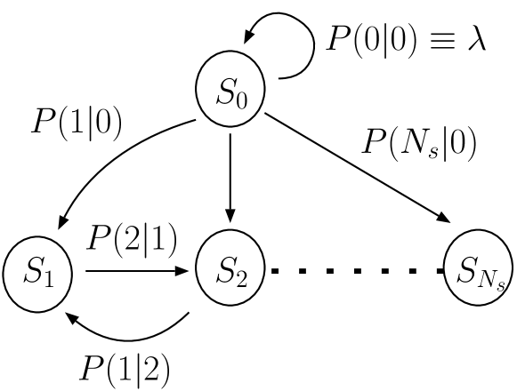
Figure 1: A Markov chain of Monte Carlo steps.

A Monte Carlo method is an implementation of a Markov process on a computer, and hence is sometimes called a Markov Chain Monte Carlo. The Monte Carlo method calculates various physical quantities by updating states of a system using random variables. These updating processes can be illustrated by a Markov chain (see the schematic in Fig. 1). Let the current state be at $S_{0}$. The states possible to move from $S_{0}$ are denoted by $S_{i}~{}(i=1,2,\cdots,N_{s})$. Define $E_{i}$ as the energy of the state $S_{i}$. The new state $S_{i}~{}(i=0,1,\cdots,N_{s})$ will be chosen with probability $P(i|0)$. One way to ensure that the system will relax to the equilibrium state is to insist that the probability $P(i|0)$ satisfies the detailed balance condition Landau .

One of the well-known ways Landau to satisfy the detailed balance condition is to use a heat-bath transition probability. In the heat-bath method, the probability $P(i|0)$ is defined to be

$$P(i|0)=\frac{\exp{(-\beta E_{i})}}{\sum_{k=0}^{N_{s}}\exp{(-\beta E_{k})}}.$$ (1)

When a system has a continuous degree of freedom, the summation of Eq. (1) becomes an integration which is generally difficult to calculate analytically.

Another popular way to satisfy the detailed balance condition is a Metropolis method. In this method, each step contains two parts; selecting a new state and accepting or rejecting the trial to move to the selected state. First, pick a state $S_{i}$ from all possible states to move to with uniform probability $1/N_{s}$. The probability $P(i|0)$ to move from $S_{0}$ to $S_{i}$ is defined to be $1$ when $\Delta E_{i}<0$, otherwise it is $\exp{\left(-\beta\Delta E_{i}\right)}$ with the energy difference $\Delta E_{i}\equiv E_{i}-E_{0}$. Therefore, the probability $P(i|0)$ in the Metropolis method is

$$P(i|0)=\left\{\begin{array}[]{cc}1/N_{s}&\mbox{if}\quad\Delta E_{i}\leq 0,\\ \exp{\left(-\beta\Delta E_{i}\right)}/N_{s}&\mbox{otherwise}.\end{array}\right.$$ (2)

When a trial is rejected, the configuration of the system is not updated. The probability $\lambda\equiv P(0|0)$ to stay in the current state after the trial is given by

$$\lambda=1-\sum_{i\neq 0}P(i|0).$$ (3)

For some parameters, e.g., under a strong external field and at an extremely low temperature, the value of $\lambda$ can be very nearly $1$. In such cases, most of computational time is spent on calculating trials which will be rejected. This rejection rate drastically decreases the efficiency of the computation. For studies of the statics of a system, the MC trial move may be changed to increase the MC efficiency Landau ; LiuLuijten . However, for studies of the dynamics a change in the MC move would change the underlying physics.

In order to overcome this problem, a rejection-free Monte Carlo (RFMC) method is proposed. It is an example of an event driven algorithm Binder ; Landau and has also been called a waiting time method MiyashitaTakano ; Jesper . Each step of the RFMC method involves first computing the time to leave the current state (the waiting time $t_{\mbox{wait}}$), and then choosing a new state to move to with the appropriate probability. It does not contain the judgment to accept or reject a trial, and, therefore, it achieves rejection-less updates of the system in each algorithmic step. The waiting time $t_{\mbox{wait}}$ is a random variable. The probability $p(t)$ to remain in the current state for $t$ steps decays exponentially as,

$$p(t)=\lambda^{t}=\exp{(t\ln{\lambda})},$$ (4)

with $\lambda$ defined in Eq. (3). Note that $\ln\lambda<0$ since $0<\lambda<1$. The time $t$ to stay in the current state is determined to be,

$$t_{\mbox{wait}}=\left\lfloor\frac{\ln r}{\ln\lambda}\right\rfloor+1,$$ (5)

where $r$ is a uniform random number on $(0,1)$ and $\lfloor x\rfloor$ denotes the integer part of $x$. The rounding down is introduced to express the discrete time step in the MC Novotny ; Munoz .

After the time of the system is advanced by $t_{\mbox{wait}}$, a new state $S_{i}$ is chosen from the all states possible to move to, except for the current state, with the probability proportional to $P(i|0)$ NovotnyPRL ; Novotny ; Munoz . Since all values of $P(i|0)$ are required to proceed one algorithm step in the RFMC, the computational cost of one step is higher than that of the normal MC. However, the waiting time $t_{\mbox{wait}}$, the time which can be advanced in one algorithmic step, can become large, for example at low temperatures, and consequently the efficiency of the RFMC can become greater than that of the standard MC.

It is worthwhile to stress that the RFMC method is mathematically equivalent to the standard MC method. Only the method of implementing the mathematics on a computer is different. Therefore, the dynamics are the same in both of the methods since they share the same Markov chain. This is in contrast to many other techniques to accelerate MC Binder , which change the underlying relationship between single-trial MC time and the motion through the phase space of the system.

III Efficiency of RFMC

In this section, we give arguments predicting the efficiency of the RFMC method in spin and hard-particle systems. The efficiency of the RFMC method is inversely proportional to the rejection rate of the standard MC. Nevertheless, the RFMC method has the same dynamics as that of the standard MC method. Therefore, the efficiency of the RFMC is related directly to the inefficiency of the standard MC.

III.1 Spin Systems

Consider a general ferromagnetic spin system with MC dynamics at low temperature with a Hamiltonian,

$${\cal H\/}=-\frac{J}{2}\sum_{\langle i,j\rangle}s_{i}s_{j},$$ (6)

with spins $s_{i}$ ($|s_{i}|=1)$ and interaction energy $J>0$. The sum is over the number of nearest-neighbor spins $n_{s}$. The expectation value of the waiting time is given by

$$\left\langle t_{\mbox{wait}}\right\rangle=\frac{1}{1-\lambda},$$ (7)

which is the reciprocal of the acceptance probability Koma . The rejection probability is $\lambda=\sum_{i}\lambda_{i}/N,$ with $N$ the number of spins. The rejection probability of a MC move where spin $i$ was the spin chosen to be changed is $\lambda_{i}$. At low enough temperature, the values of $\lambda_{i}$ are almost identical and any changes will usually involve an energy increase, since all of the spins are almost parallel. Accordingly, the expectation value of $\lambda_{i}$ can be written as

$$\left\langle\lambda_{i}\right\rangle=1-\left\langle\mbox{e}^{-\beta\Delta E}\right\rangle_{\mbox{sc}},$$ (8)

where $\beta$ is the inverse temperature, $\Delta E$ is the energy difference between the current state and the chosen trial state and $\left\langle\cdots\right\rangle_{\mbox{sc}}$ denotes the average for all possible spin configurations. With Eqs. (7), and (8), the expectation value of the waiting time is approximated by

$$\left\langle t_{\mbox{wait}}\right\rangle=\frac{1}{\left\langle\mbox{e}^{-\beta\Delta E}\right\rangle_{\mbox{sc}}}.$$ (9)

The approximation involves replacing the expectation value of a function by the function of the expectation value, which is a mean-field or asymptotic type of approximation. Equation (9) implies that the waiting time, which is the efficiency of the RFMC method, is inversely proportional to the probability that the trial to flip a randomly chosen spin is accepted. Note that, the above argument depends only on the details of the spins, not on the lattice type or dimension of the system. In the following, we evaluate Eq. (9) for three specific cases.

III.1.1 Ising Model

In the Ising model case, the energy difference $\Delta E$ is just $n_{s}J$ with a number of neighbor spins $n_{s}$. The expectation value of the acceptance probability is $\left\langle\mbox{e}^{-\beta\Delta E}\right\rangle_{\mbox{sc}}=\mbox{exp}({-n_{s}J\beta}),$ and therefore, the waiting time is

$$\left\langle t_{\mbox{wait}}\right\rangle\sim\mbox{exp}({n_{s}J\beta}),$$ (10)

which shows that the efficiency of the RFMC will increase exponentially as the temperature decreases. Similarly, for other systems with discrete degrees of freedom, such as the q-state Potts or clock models, $t_{\mbox{wait}}$ increases exponentially with $\beta$ Novotny .

III.1.2 Classical XY Model

When the spin has continuous degrees of freedom, the average in Eq. (9) becomes an integration. For the classical XY model, the expectation value of the acceptance probability becomes,

$$\left\langle\mbox{e}^{-\beta\Delta E}\right\rangle_{\mbox{sc}}=\frac{1}{\pi}\int_{0}^{\pi}\mbox{d}\theta\mbox{e}^{-n_{s}J\beta(1-\cos\theta)},$$ (11)

since the energy increase $\Delta E=n_{s}J(1-\cos\theta)$ with the angle of the spin $\theta$. When $\beta\gg 1$, the integrand has a value only around $\theta\sim 0$. Therefore we make a saddle point approximation $\cos\theta\sim 1-\theta^{2}/2$, and change the upper limit of the integration to infinity. Then Eq. (11) reduces to the Gaussian integral,

$$\left\langle\mbox{e}^{-\beta\Delta E}\right\rangle_{\mbox{sc}}\sim\frac{1}{\pi}\int_{0}^{\infty}\mbox{d}\theta\mbox{e}^{-n_{s}J\beta\theta^{2}/2}=\frac{1}{\sqrt{2\pi n_{s}J\beta}}.$$ (12)

With Eqs. (9) and (12), we have,

$$t_{\mbox{wait}}\sim\sqrt{2\pi n_{s}J\beta}.$$ (13)

Therefore, the efficiency of the RFMC method grows less rapidly with decreasing temperature in the XY model than it does for a discrete spin model. Nevertheless, at low enough temperature the RFMC will still outperform the standard dynamic MC.

III.1.3 Classical Heisenberg Model

For the classical Heisenberg spin model, the energy difference $\Delta E(\theta,\phi)=n_{s}J(1-\cos\theta)$, which is equivalent to the XY model. The expectation value of the acceptance probability is obtained from the integration,

$$\left\langle\mbox{e}^{-\beta\Delta E}\right\rangle_{\mbox{sc}} = \frac{1}{4\pi}\int_{0}^{2\pi}\!\!\!\!\!\!\!\mbox{d}\phi\int_{0}^{\pi}\!\!\!\!\!\!\mbox{d}\theta\sin\theta\cdot\mbox{e}^{-n_{s}J\beta(1-\cos\theta)}$$ (14)

$$= \frac{1-\mbox{e}^{-2n_{s}J\beta}}{2n_{s}J\beta}.$$

Therefore,

$$\left\langle t_{\mbox{wait}}\right\rangle=\frac{2n_{s}J\beta}{1-\mbox{e}^{-2n_{s}J\beta}}\sim 2n_{s}J\beta,$$ (15)

since $\mbox{e}^{-2n_{s}J\beta}\ll 1$. This result, that the efficiency is proportional to $\beta$, agrees with the past RFMC study Munoz . As the temperature is lowered, the efficiency of the RFMC for the classical Heisenberg spin model grows more rapidly than for the XY model, but not as rapidly as for a discrete spin model.

III.2 Hard Particle Systems

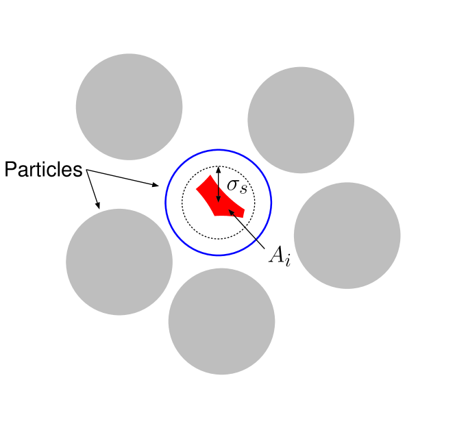
Figure 2: (Color online) A schematic drawing of the definition of $A_{i}$ (shaded). The solid circles are particles and the small dashed circle has a radius $\sigma_{s}$. The shaded area is the area which is a continuous set of the points that the center of the chosen particle can move to. The ratio of $A_{i}$ to the area of the trial circle $\pi{\sigma_{s}}^{2}$ gives the probability of accepting the move, $1-\lambda_{i}$, given that the center particle has been chosen as the one to move.

Next, consider a hard-disk (HD) system with $N$ particles. A dynamic Monte Carlo procedure based on an underlying random-walk dynamics is: 1) choose one particle randomly [from a uniform distribution over the index of all $N$ particles], 2) choose a new position for the center of this chosen particle. The new position is chosen uniformly in the circle of radius $\sigma_{s}$, called a step length, centered on the original position of the particle. This trial move is accepted when the new position has no overlap with any other particle, otherwise, the trial move is rejected. One MC step involves $N$ trials, and the time evolution of this system can be considered to be Brownian-motion with a diffusion constant $D\propto\sigma_{s}^{2}$ for a low particle density. The probability $\lambda_{i}$, which is the probability that the Monte Carlo trial of particle $i$ is rejected, is

$$\lambda_{i}=1-\frac{A_{i}}{\pi{\sigma_{s}}^{2}},$$ (16)

with $A_{i}$ the area particle $i$ can move within $\sigma_{s}$ without any overlap (see Fig. 2). The rejection probability $\lambda$ is $\lambda=1-\left\langle A\right\rangle/\pi\sigma_{s}^{2},$ with the average of area $\left\langle A\right\rangle\equiv\sum_{i}A_{i}/N$. The mean distance between two neighboring particles is $2a$ and the radius of the particle is $\sigma$. The radius of the area in which the particle can move is of order $(a-\sigma)$ (see Fig. 3). Therefore,

$$A_{i}\sim(a-\sigma)^{2}.$$ (17)

The density, $\rho$, of the system is inversely proportional to $a^{2}$ with the fixed radius $\sigma$, and $\rho$ becomes the closest packing density $\rho_{\mbox{\small cp}}$ when $a\rightarrow\sigma$. Therefore, we have

$$\frac{\rho}{\rho_{\mbox{\small cp}}}=\frac{\sigma^{2}}{a^{2}}.$$ (18)

From Eqs. (17) and (18), the behavior of $A_{i}$ is expected to be

$$A_{i} \sim (\sqrt{\rho_{\mbox{\small cp}}}-\sqrt{\rho})^{2}$$ (19)

$$\sim \varepsilon^{2},$$

with $\varepsilon\equiv(\rho_{\mbox{\small cp}}-\rho)/\rho_{\mbox{\small cp}}$, the result being valid for $\rho$ near $\rho_{\mbox{\small cp}}$. We thus obtain the expected value of the waiting time for the HD system to be,

$$\left\langle t_{\mbox{wait}}\right\rangle\sim\left(\frac{\sigma_{s}}{\varepsilon}\right)^{2}.$$ (20)

Similar arguments give $\left\langle t_{\mbox{wait}}\right\rangle$ for a $d$-dimensional hard particle system,

$$\left\langle t_{\mbox{wait}}\right\rangle\sim\left(\frac{\sigma_{s}}{\varepsilon}\right)^{d}.$$ (21)

Note that the behavior of $\left\langle t_{\mbox{wait}}\right\rangle$ depends on the dimension in the particle systems, while that of the spin systems does not.

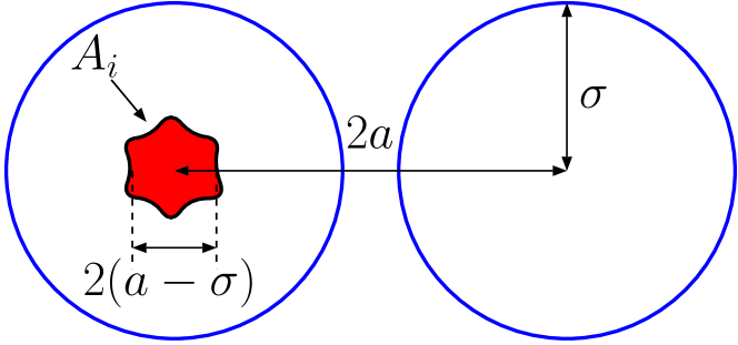
Figure 3: (Color online) A schematic drawing of $A_{i}$. The radius of the particles and mean distance between centers of neighboring particles are denoted by $\sigma$ and $2a$, respectively. The ‘radius’ of area $A_{i}$ is on the order of $(a-\sigma)$, and hence $A_{i}\propto(a-\sigma)^{2}$.

III.3 Simulations

III.3.1 Waiting Time

In order to confirm our predictions, Monte Carlo simulations were performed on two- and three-dimensional Ising, XY, and Heisenberg spin systems on a square lattice ($d=2$) and a simple cubic lattice ($d=3$). The linear system size simulated is $L=128$, and periodic boundary conditions are used in all directions. After thermalization of $10^{4}$ MC steps per spin from the perfectly ordered state, the number of rejected trials $N_{r}$ and the total trials $N_{t}$ are counted over $10^{3}$ MC steps per spin; therefore, $N_{t}=128^{d}\cdot 10^{3}$ with the dimension of the system $d$. Then the rejection probability $\lambda$ is approximated by $\lambda\sim N_{r}/N_{t}$. Using this $\lambda$, we estimated the value of $\left\langle t_{\mbox{wait}}\right\rangle$. The simulation results are shown in Fig. 4. The graphs show good agreement with our arguments. It is also worth noting that the prefactors we found are the same (within statistical errors) for the two- and three-dimensional systems.

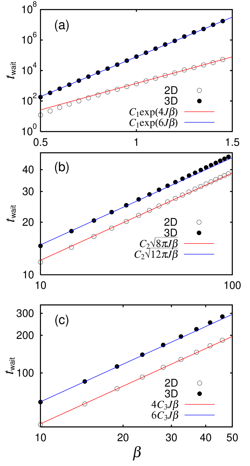
Figure 4: (Color online) The waiting times $t_{\mbox{wait}}$ vs. $\beta$ on square lattices and simple-cubic lattices of (a) Ising, (b) XY, and (c) Heisenberg spin systems. Decimal logarithms are taken for the vertical axis of (a) and both axes of (b) and (c). Open circles are the calculated waiting time and solid lines are the predicted behavior with $C_{1}=0.48$, $C_{2}=0.54$, and $C_{3}=0.49$. The number of neighboring spins $n_{s}=4$ for the two-dimensional and $n_{s}=6$ for the three-dimensional systems. They show excellent agreement with the predictions.

The behavior of the waiting time in the hard-particle systems is also confirmed. Monte Carlo simulations were performed on HD system with $N=23288$ and the hard-sphere (HS) system with $N=4000$. After $10^{4}$ MC steps per particle, the value of $\left\langle t_{\mbox{wait}}\right\rangle$ is estimated from $10^{4}$ MC steps per particle. The results are shown in Fig. 5, in good agreement with our predictions.

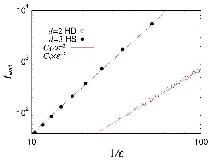
Figure 5: (Color online) The waiting time $t_{\mbox{wait}}$ of the hard-disk (HD) and hard-sphere (HS) systems at high densities. They are shown as functions of $1/\varepsilon$ with $\varepsilon\equiv(\rho_{\mbox{\small cp}}-\rho)/\rho_{\mbox{\small cp}}$. Decimal logarithms are taken for both axes. The solid lines are for visual reference with $C_{4}=0.07$ and $C_{5}=0.04$, respectively. This shows that the waiting time behaves as $\sim\varepsilon^{-d}$ with the dimension of the system $d$.

III.3.2 Efficiency

To further test our arguments, we implement the RFMC for the classical XY spin system. We discretize the spin state and use the 128-state clock model since we cannot calculate an acceptance probability analytically in this system. We confirmed that the behavior of the system with discretized spins is equivalent to the system with a continuum degree of freedom in the region where we simulated. At very low temperatures (lower than we simulated), where the number of states in the clock model approximation becomes important, we expect that the RFMC efficiency crosses over to an exponential dependence as predicted in Eq. (10). The system size is $128\times 128$ and periodic boundary conditions are taken along the both directions. Measurements are started after $10^{5}$ MC steps. The CPU-time ratio of the standard MC to the RFMC methods to achieve $1000$ accepted MC trials is shown in Fig. 6. The behavior of the efficiency of the RFMC is as predicted in Eq. (13).

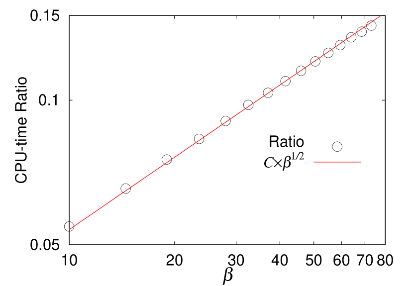
Figure 6: (Color online) The ratio of the required computational time to achieve $10^{3}$ accepted MC trials of the standard MC to the RFMC method in the classical XY spin system. Decimal logarithms are taken along both axes. The solid line is for visual reference ($C=0.017$). The efficiency of the RFMC behaves as predicted.

IV Application to hard-disk systems

Consider a hard disk system with $N$ particles all with the radius $\sigma$. Now that the high density expected efficiency of the RFMC for hard particle algorithms has been obtained, an actual RFMC implementation for hard particles should be implemented. This section describes such an implementation. The standard MC method for the system involves choosing a particle, and trying to move the chosen particle within a circle with radius $\sigma_{s}$ centered on the original position of the chosen particle. To apply a RFMC method to the hard-disk system, define $\lambda_{i}$ as the probability that a trial to move particle $i$ is rejected (given that particle $i$ was chosen as the particle to attempt a move). Using the definition of $\lambda_{i}$, we can construct the algorithm of the RFMC method for the hard-disk system as follows:

1. Calculate the waiting time $t_{\mbox{wait}}$ using Eq. (5) with $\lambda=\frac{1}{N}\sum_{i}\lambda_{i}$.

2. Advance the time of the system by $t_{\mbox{wait}}$.

3. Choose a particle $i$ with the probability proportional to $1-\lambda_{i}$, which is the probability that (given that particle $i$ was the particle chosen for an attempted move) the trial to move the particle $i$ would be accepted.

4. Choose the new position of the chosen particle $i$ uniformly from all the points to which the particle $i$ is allowed to move.

The steps described above are the same as the RFMC for continuous spin systems Munoz , but the algorithms to calculate $\lambda_{i}$, to choose a particle to move and to determine a new position of the chosen particle are unique to the hard-disk system. In the following, we describe the details of the algorithms.

IV.1 Calculation of $A_{i}$

The area $A_{i}$ is the continuous set of positions in which the particle can be placed without any overlaps. Without neighboring particles, the shape of $A_{i}$ would be a filled circle with a radius $\sigma_{s}$. Let’s call it a trial circle. In the general case, the shape of $A_{i}$ is the remaining part of the trial circle after removing the overlap of ‘shadows’ of neighboring particles. The shape of the shadow is a circle with a radius $2\sigma$ which is concentric to a neighboring particle. Let’s call this a shadow circle. The area $A_{i}$, thus, consists of areas of arcs of a trial circle and that of shadow circles.

To compute the value of $A_{i}$, we develop a method we call the survival point method. See Fig. 7 (a). The chosen particle is shown as a solid circle, the trial circle is shown as a concentric dashed circle, and the area $A_{i}$ is the shaded region. Each neighboring particle (filled circles) has a shadow circle which is concentric and has radius $2\sigma$. An enlargement of the area $A_{i}$ is shown in Fig. 7 (b). It is seen that in this example this area has five vertices which are intersection points of shadow particles, we call them survived vertex points. In Fig. 7 (c), these survived vertex points are shown as small filled circles. Straight lines connect the center of the chosen particle and the intersection points. In this case the area $A_{i}$ is divided into five portions.

Each divided figure is the remaining part of an isosceles triangle with the overlap of a shadow circle removed. It is easy to calculate this area. Thus, all we have to do is to find all survived vertex points which form the area $A_{i}$. First, make a list of all intersection points of shadow circles and the trial circle. Next, remove points which are included in other shadow circles from the list, since these points cannot be vertices forming the area $A_{i}$. After this removal process, we have the vertices which form the area $A_{i}$ (see Fig. 7 (c)). The calculation process of a partial figure which forms $A_{i}$ is shown in Fig. 7 (d). The vertices are denoted by $P_{1}$ and $P_{2}$, and the center of the shadow circle is denoted by $S$. The survived vertices $P_{1}$ and $P_{2}$ are on the shadow circle centered at $S$, so $\overline{SP_{1}}=\overline{SP_{2}}=2\sigma$. The area of $OP_{1}SP_{2}$ can be calculated by summing the two triangles $OP_{1}P_{2}$ and $SP_{1}P_{2}$ with Heron’s formula. The area of the chord is $4\sigma^{2}\theta$. Finally the portion of the area $O{P_{1}}{P_{2}}$ is calculated by subtracting the area of the chord $S{P_{1}}{P_{2}}$ from the area of the quadrilateral $OP_{1}SP_{2}$. The total area $A_{i}$ is the sum of one such calculation for each survived vertex.

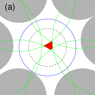
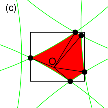
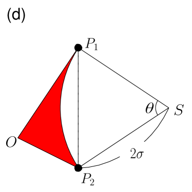
Figure 7: (Color online) Computation of the value of $A_{i}$. (a) Filled gray circles represent neighboring particles with radius $\sigma$ and large circles are shadows of them (we call them ‘shadow circles’) with radius $2\sigma$. (b) An enlargement. The shaded area is the area into which the particle $i$ is allowed to move. This figure is made by removing overlaps of shadow circles from the trial circle of radius $\sigma_{s}$ centered on the chosen particle. (c) The survived vertex points. The center of the trial circle is denoted by $O$. The solid circles represent survived vertex points, which form the area $A_{i}$. With them, we can calculate the value of $A_{i}$. The rectangle denotes a bounding rectangle. Each two adjacent survived vertex points and the center point O form a triangle. In this example there are five survived vertex points, and consequently five triangles to consider. (d) To calculate a portion of $A_{i}$, the area within each triangle formed by survived vertex points and O is calculated. The survived vertex points are the intersection points of the shadow circles or the trial circles, and here are denoted by $P_{1}$ and $P_{2}$. The center of the shadow particle is $S$. To find the shaded area a Monte Carlo procedure is performed in the shaded area of either (c) or (d), and only survived points generated in the shaded area are used as the new location for the new point O.

IV.2 Choosing a particle to move

After calculation of $t_{\mbox{wait}}$ and advancing the time of the system by it, we have to choose a particle $i$ to move with a probability proportional to $1-\lambda_{i}$. With a direct implementation, i.e., with the integration scheme IntegrationSearch , the order of the computation is $O(N)$, which is very time consuming. Other approaches are proposed like a three level search for spin systems threelevel . The three-level search improves the efficiency of the search by determining coordinates of a spin to update one by one. However, it is difficult to apply this method for particle systems, since neighbors of particles are not fixed. Here we use a complete binary tree search for the choosing part of the algorithm.

First, calculate the area $A_{i}$ for each of the particles. Since an acceptance probability $1-\lambda_{i}$ is proportional to $A_{i}$ as shown in Eq. (16), the particle should be chosen with the probability proportional to $A_{i}$.

Next, construct a complete binary tree as follows,

1. Prepare a complete binary tree with enough height $h$, this height $h$ should satisfy $2^{h-2}<N\leq 2^{h-1}$.

2. Label each node with $T_{n}^{k}$, which denotes the $n^{\rm th}$ value at level $k$. The root node is labeled by $T_{1}^{h}$. A node labeled $T_{n}^{k+1}$ has branches leading to two nodes $T_{2n-1}^{k}$ and $T_{2n}^{k}$.

3. Associate every bottom node $T_{i}^{1}$ with the value of area $A_{i}$. If the number of bottom nodes $2^{h-1}$ is larger than $N$, the rest of the nodes are associated with zero, namely, $T_{i}^{1}=0~{}(i>N)$.

4. Associate nodes at higher levels ($k>1$) recursively with the sum of the values associated with its two children, namely, $T_{n}^{k+1}=T_{2n-1}^{k}+T_{2n}^{k}$.

A sample of a compete binary tree is shown in Fig. 8. Each node has the value $T_{n}^{k}$ and the value of each node at level $k+1$ is the sum of the values of its two children nodes at level $k$. The root node, which is $T_{1}^{4}$ in Fig. 8, has the sum of all $A_{i}$, that is,

$$T_{1}^{h}=\sum_{i}^{N}A_{i}.$$ (22)

Using this tree, we can choose a particle with the probability proportional to $A_{i}$ in the following way.

1. $k\leftarrow 1$, $i\leftarrow 1$.

2. Prepare a random number $r$ uniform on $(0,T_{i}^{k})$.

3. $\left\{\begin{array}[]{lc}i\leftarrow 2i-1&\quad\mbox{if}\quad r<T_{2i-1}^{k-1}\\ i\leftarrow 2i&\quad\mbox{otherwise}\end{array}\right.$

4. $k\leftarrow i-1$.

5. if $k>1$ then go to 2

Consequently, choosing the bottom node requires $h-1$ random numbers.

After the above processes, the final value of $i$ indicates the index of the particle to move. The order of this search algorithm is $O(\log N)$. When the position of particle $i$ is moved, the value of $A_{i}$ is also modified. We only have to update part of this tree for the chosen particle and its neighbors. The order of this update is also $O(\log N)$, which is much faster than $O(N)$ of the direct implementation. Details to implement the complete binary tree search method are described in the appendix.

Figure 8: A complete binary tree search. An example of $N=8$ ($h=4$) is shown. The value of a node $T_{i}^{k}$ is the sum of the values of its two child nodes, namely, $T_{i}^{k}=T_{2i}^{k-1}+T_{2i-1}^{k-1}$. After construction of the tree, we use $h-1$ random numbers to choose a bottom node. This bottom node is associated with the index of the particle that will be moved in this algorithmic step of the RFMC method.

IV.3 Find a new position of the particle

After choosing a particle, we have to choose the new position for it. It is difficult to choose a point uniformly from the points allowed to move into, since its shape is generally very complicated (see Fig. 2). Therefore, we have chosen to choose the new position using a Monte Carlo rejection method. Namely we generate a random position uniformly over some bounding area that includes all of the area $A_{i}$. [Such as the dashed circle of radius $\sigma_{s}$ in Fig 7(a) or the rectangle in Fig 7(c).] If this point is not in $A_{i}$ it is rejected and another uniformly distributed random point over the bounding area is generated. The first point not to be rejected is the new position of the particle, since it is in the area $A_{i}$, and this point is used as the new center for the particle. Finally, the new $A_{i}$ value for the chosen particle and all of its neighboring particles must be recalculated. This completes one algorithmic step of the RFMC method.

The typical value of area $A_{i}$ is very small compared to the trial circle at high density, and hence the Monte Carlo trial to find the new position of the particle to be moved became very inefficient. To improve this, it is effective to limit the trial area for the Monte Carlo by making the bounding area very close to the area $A_{i}$. We outline two different survived point methods, but have only implemented the first.

For the first method, the one actually implemented in this paper see Fig. 7 (c). The solid rectangle is a bounding rectangle which includes the area $A_{i}$. It is easy to obtain the bounding rectangle with the survived vertex points. With the set of survived vertex points $\{(x_{i},y_{i})\}$, a diagonal line of the bounding rectangle is from $(\min{\{x_{i}\}},\min{\{y_{i}\}})$ to $(\max{\{x_{i}\}},\max{\{y_{i}\}})$. Then we can perform Monte Carlo trials for a new position within only this rectangle. The area of the rectangle is on the same order of $A_{i}$, so the probability of success to obtain the new position is drastically improved compared with the direct search over the trial circle.

An alternative method is to first use a random number to decide which of the triangles formed with point O and two adjacent survived vertex points the survived point will fall into. This is done analytically since the areas of each triangle with removed shadow circle chords have been already calculated. Then the shortest side formed with point O and the two survived vertex points (say $\overline{SP_{2}}$ in Fig. 7 (d)) is lengthened to be equal to the longest side ($\overline{SP_{1}}$ in Fig. 7 (d)). The random trial point is then generated within the section of the circle with a radius equal to the longest side ($\overline{SP_{1}}$ in Fig. 7 (d)). Then the point becomes the survived point used for the new location of point O if the trial point is within the shaded area. Otherwise, this procedure repeats in the same extended circular section until a survived point is found.

IV.4 Simulation

IV.4.1 Calculation of $A_{i}$

In order to test our method to calculate $A_{i}$ described in Sec. IV.1, the values of $A_{i}$ were also evaluated by a Monte Carlo sampling ($A_{\rm MC}$) with trial points uniformly drawn over the trial circle. The density of the system $\rho$ is defined to be $\rho=4N\sigma^{2}/L^{2}$ with the number of particles $N$, the radius of the particles $\sigma$ and the linear system size $L$, respectively. Throughout this study, the number of particles $N$ is set to be $23288$ and periodic boundary conditions are taken for both axes. The number of the generated configurations were 3000, and $10^{6}$ MC trial points are taken for each of the configurations to evaluate its area. The density of the system is fixed at $\rho=0.9$. The result is shown in Fig. 9. The area $A_{i}$ is normalized by the area of the trial circles (see Fig. 2). The difference between the MC and our survived point method is less than $0.01\%$ for all areas, which is the same order as the statistical error of our MC method. The standard deviation of the MC area calculation is determined by dividing the data into 10 groups, each including $10^{5}$ samples. This result shows that the value of $A_{i}$ is properly calculated by our method.

Figure 9: Comparison of calculated $A_{i}$ between our survived points method and that calculated by a more straightforward MC method. Units on both axes are dimensionless. The circles denote the ratio of $A_{\mbox{RFMC}}$ to the $A_{\mbox{MC}}$. The number of configurations is $3000$ at $\rho=0.9$ and $10^{6}$ independent samples are averaged for each configuration. The solid lines are the standard deviation obtained from the jack-knife procedure described in the text.

IV.4.2 Time evolution

The dynamics of the standard MC and of the RFMC must be the same. To test this in our case, we observed the time evolution of the six-fold bond-orientational order parameter $\phi_{6}$ HalperinNelson . The parameter $\phi_{6}$ is defined to be

$$\phi_{6}=\left<\exp(6i\theta)\right>,$$ (23)

with the bond angle $\theta$ which has a definition described in Fig. 10. The average is taken for all pairs of neighboring particles. The parameter $\phi_{6}$ becomes 1 when all particles are located on the points of a hexagonal grid, and it becomes $0$ when the particle location is completely disordered. Therefore $\phi_{6}$ describes how close the system is to the perfect hexagonal packing. The neighbors in an off-lattice model are strictly defined with the Voronoi construction Jaster , which is a very time-consuming method. In this paper, two particles separated by a distance less than $2.6\sigma$ are defined as neighbors. We confirmed that the value of $\phi_{6}$ is approximately the same value as the value obtained with the Voronoi construction.

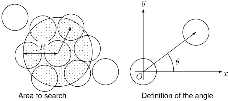
Figure 10: The definition of the neighboring particles and bond angle $\theta$. Two particles separated by a distance less than $R$ are defined as neighbors. Here, $R$ is set to be $2.6\sigma$ with the radius $\sigma$ of particles. The bond angle $\theta$ is defined to be an angle between the bond connecting neighboring particles with respect to an arbitrary, but fixed global axis.

At the beginning of the simulation, the particles are set up in a perfect hexagonal order, namely, $\phi_{6}(t=0,\rho)=1$. The order parameter $\phi_{6}$ starts to relax to the value of the equilibrium state. With this nonequilibrium relaxation (NER) behavior of order parameters, critical points and critical exponents of various phase transitions can be determined accurately ItoPhysica1 ; ItoPhysica2 ; ItoMastuhisa ; ItoHukushima . This method is called a NER method. Watanabe et al. Watanabe ; Watanabe2 studied two-dimensional melting based on the NER method for the Kosterlitz-Thouless transition NERKT by observing the relaxation behavior of $\phi_{6}$. Therefore, the following time evolutions of $\phi_{6}$ contains information about the two-dimensional melting transition.

Time evolutions of $\phi_{6}$ are shown in Fig. 11. Solid lines are results of the standard MC simulation and symbols (circles, triangles and squares) are the results of the RFMC. Fig. 11 shows that both behaviors are equivalent for the two methods. This is essentially a check of the program implementation, since the physical dynamic is the same for both the MC and the RFMC methods.

Figure 11: Relaxation behaviors of the bond-orientational order. Solid lines are the results of the standard MC and symbols (circles, triangles and squares) are the results of the RFMC. The data intervals between accepted updates for the RFMC algorithm becomes longer at high density, while the data keeps the behavior of the standard MC algorithm.

IV.4.3 Efficiency

Figure 12: (a) The required computational time to achieve 1000 acceptances of the Monte Carlo moves with the standard MC (open circles) and the RFMC (solid circles). (b) CPU-time ratio vs. $1/\varepsilon$ with $\varepsilon\equiv(\rho_{\mbox{\small cp}}-\rho)/\rho_{\mbox{\small cp}}$. Decimal logarithms are taken for both axes. The solid line is drawn for the visual reference ($C=0.9\times 10^{-3}$).

The computational times required to achieve $1000$ accepted MC steps are shown in Fig. 12(a). Configurations are started from the perfect hexagonal configuration and both measurements are started after $10^{6}$ MC steps. All simulations are performed on an Intel Xeon $2.4$ GHz computer. While the computational time of the RFMC (open circles) is almost constant, a longer computational time is required for the standard Monte Carlo (solid circles) at higher density. It shows that the RFMC is more efficient at high densities, in spite of the additional bookkeeping involved in the RFMC method (so one RFMC algorithmic step takes much longer than one standard MC step).

The CPU-time ratio of the standard MC to the RFMC is shown in Fig. 12(b). The data are shown as a function of $1/\varepsilon$, where $\varepsilon\equiv(\rho_{\mbox{\small cp}}-\rho)/\rho_{\mbox{\small cp}}$, the closest density is $\rho_{\mbox{\small cp}}$ and the density of the system is $\rho$. The CPU-time ratio, which is the efficiency of the RFMC compared to that of the standard MC, diverges as $\varepsilon^{-2}$. This confirms the predicted behavior of Eq. (21).

V Summary and Discussion

We predicted the behavior of the average waiting time $\left\langle t_{\mbox{wait}}\right\rangle$ to be

$$\left\langle t_{\mbox{wait}}\right\rangle\sim\left\{\begin{array}[]{cl}\exp\left({\rm const.}\>\beta\right)&\left(\begin{array}[]{l}\mbox{Ising and other discrete}\\ \mbox{spin systems}\end{array}\right)\\ \sqrt{\beta}&\mbox{(classical XY)}\\ \beta&\mbox{(classical Heisenberg)}\\ \varepsilon^{-d}&\mbox{(hard-particle)}\end{array}\right.,$$ (24)

for the efficiency of the RFMC method. These have been confirmed by our MC simulations. It is interesting that the behavior of the HD system in the high density regime is different from that of the XY spin system at low temperature, while the phase transition of both are of a Kosterlitz-Thouless-type HalperinNelson ; NERHD ; OI03AB (see for a review Ref. Strandburg ). Our arguments for $\left\langle t_{\mbox{wait}}\right\rangle$ are very general, and consequently should be able to give the RFMC efficiency for other models, for example, a discrete stochastic model Gillespie .

We implemented the rejection-free Monte Carlo algorithm for the hard-disk system. This method conserves the property of the dynamic behavior of the original Monte Carlo method. In other words, the time scales will not depend on the density, but are rather set by some Brownian-motion type of dynamic for all densities. An estimate of the time scales between the MC and physical time can thus be obtained by setting the mean-free path of an isolated particle to be proportional to the value $\sigma_{s}$. Note that strictly this is only true in the limit $\sigma_{s}\rightarrow 0$, but it should be a reasonable approximation for a small finite $\sigma_{s}$.

We also find that for a fixed value of $\sigma_{s}$, the RFMC method is more efficient at high density. Therefore, the RFMC method should be useful for studies of two-dimensional solids or studies of high-density glass materials, while the efficiency of the RFMC is less than that of the standard method at the critical point. It may also be possible to make the algorithm even more efficient by further optimization techniques, e.g., by utilizing the ideas of absorbing Markov chains (for the MCAMC method for discrete state spaces see Novotny and references therein). Increased algorithmic efficiencies for the Monte Carlo dynamics of hard disks could be useful to further test physical phenomena using hard disk systems, such as for example the relationship between fluctuations and dissipation of work in a Joule experiment Cleuren .

The RFMC method gives the same dynamics as the standard MC method, and consequently, the RFMC method allows one in certain regimes to efficiently study the dynamical behavior of systems with a given physical MC dynamic. The dynamic for a MC has been derived from underlying physical properties for some systems Mart77 ; Park1 ; Okabe . It has been shown that using different MC dynamics can have enormous consequences on physical properties such as on low-temperature nucleation Park2 ; Buendia . Consequently, this equivalence between the two MC methods is essential.

Appendix

Figure 13: Implementation of the complete binary tree search with an array. The required size of the array to implement the tree with height $h$ is $2^{h}-1$. The height $h$ should satisfy $2^{h-2}<N\leq 2^{h-1}$. When the number of particles $N$ is $2^{h-1}$, which is the maximum number of particles that the tree with height $h$ can treat, the size of the array is $2N-1$.

The complete binary tree search can be implemented with an one-dimensional array. To make it simple, let the number of particles $N$ be $2^{h-1}$. The tree with height $h$ requires an array $a(i)$ with size $2N-1$. First, associate each bottom node with a corresponding value as

$$a(N+i-1)\leftarrow A_{i}\quad(i=1,2,\cdots,N),$$ (25)

which corresponds to $T_{i}^{1}\leftarrow A_{i}$. Next, associate parent nodes recursively as

• $i\leftarrow N$

• While $i\neq 0$

• $a(i)\leftarrow a(2i)+a(2i+1)$

• $i\leftarrow i-1$

• next $i$

Using this array, we can pick particle $i$ with the probability proportional to $A_{i}$ as,

• $i\leftarrow 1$

• While $i<N$

• Prepare a uniform random number $r$ on $(0,a(i))$

• $\left\{\begin{array}[]{ll}i\leftarrow 2i&\quad\mbox{if}\quad r<a(2i)\\ i\leftarrow 2i+1&\quad\mbox{otherwise}\end{array}\right.$

• next $i$

• $i\leftarrow i-N+1$.

After the above procedure, we obtain the index $i$ of the chosen particle. When the value of $A_{i}$ is changed, the tree should be updated. The update process is as follows,

• $a(N+i-1)\leftarrow A_{i}$

• $i\leftarrow\left\lfloor\displaystyle\frac{i+N}{2}\right\rfloor$

• While $i\neq 1$

• $a(i)\leftarrow a(2i)+a(2i+1)$

• $i\leftarrow\left\lfloor\displaystyle i/2\right\rfloor$

• next $i$.

Note that, when the chosen particle is moved, the acceptance probabilities of the neighboring particles of the moved particle are also changed. Therefore, we have to perform the above process for all neighboring particles.

References

- (1) K. Binder, Monte Carlo Methods in Statistical Physics, ed. K. Binder, (Springer, Berlin, 1979).
- (2) D. Landau and K. Binder, A Guide to Monte Carlo Simulations in Statistical Physics, 2nd Ed. (Cambridge, 2005).
- (3) J. Hausmann and P. Ruján, Phys. Rev. Lett. 79, 3339 (1997); P.B. Sunil Kumar, G. Gompper, and R. Lipowsky, Phys. Rev. Lett. 86, 3911 (2001); D. Chowdhury, D. Stauffer, and A. Kunwar, Phys. Rev. Lett. 90, 068101 (2003).
- (4) A. B. Bortz, M. H. Kalos and J. J. Lebowitz, J. Comput. Phys 17, 10 (1975).
- (5) S. Miyashita and H. Takano, Prog. Theor. Phys. 63 797 (1980).
- (6) M. A. Novotny in Annual Reviews of Computational Physics IX, editor D. Stauffer (World Scientific, Singapore, 2001), p. 153.
- (7) J. D. Muñoz, M. A. Novotny and S. J. Mitchell, Phys. Rev. E 67, 026101 (2003).
- (8) B. I. Halperin and D. R. Nelson, Phys. Rev. Lett. 41, 121 (1978);A. P. Young, Phys. Rev. B 19, 1855 (1979).
- (9) H. Watanabe, S. Yukawa, and N. Ito, Phys. Rev. E, 71, 016702 (2005).
- (10) S. Wang, S.J. Mitchell, and P.A. Rikvold, Comp. Mater. Sci., 29, 145 (2004).
- (11) H. Watanabe, S. Yukawa, and N. Ito, submitted to Phys. Rev. E.
- (12) J. Liu and E. Luijten, Phys. Rev. Lett. 92 035504 (2004).
- (13) J. Dall and P. Sibani, Comp. Phys. Commun. 141 260 (2001).
- (14) M. A. Novotny, Phys. Rev. Lett. 74, 1 (1995); erratum 75 1424 (1995).
- (15) T. Koma, J. Stat. Phys. 71, 269 (1993).
- (16) The order of the search itself is in the direct implementation with the integration scheme, since we can use a binary search for an ordered list. However, when one value is modified, the order of the computation to update the list of values is .
- (17) J. L. Blue, I. Beichl, and F. Sullivan, Phys. Rev. E 51, R867 (1995).
- (18) A. Jaster, Phys. Rev. E 59, 2594 (1999).
- (19) N. Ito, Physica A 192 (1993) 604.
- (20) N. Ito, Physica A 196 (1993) 591.
- (21) N. Ito, T. Matsuhisa and H. Kitatani, J. Phys. Soc. Jpn. 67 (1998) 1188.
- (22) N. Ito, K. Hukushima, K. Ogawa and Y. Ozeki, J. Phys. Soc. Jpn. 69 1931 (2000).
- (23) H. Watanabe, S. Yukawa, Y. Ozeki and N. Ito, Phys. Rev. E 66, 041110 (2002).
- (24) H. Watanabe, S. Yukawa, Y. Ozeki, and N. Ito, Phys. Rev. E, 69, 045103(R) (2004).
- (25) Y. Ozeki, K. Ogawa and N. Ito, Phys. Rev. E, 67, 026702 (2003).
- (26) H. Watanabe, S. Yukawa, Y. Ozeki, and N. Ito, Phys. Rev. E 66, 041110 (2002);
- (27) Y. Ozeki, K. Ogawa, and N. Ito, Phys. Rev. E 67, 026702 (2003); Y. Ozeki and N. Ito, Phys. Rev. B 68, 054414 (2003).
- (28) K.J. Strandburg, Rev. Mod. Phys. 60, 161 (1988).
- (29) B.T. Werner and D.T. Gillespie, Phys. Rev. Lett. 71, 3230 (1993).
- (30) B. Cleuren, C. van den Broeck, and R. Kawai, Phys. Rev. Lett. 96, 050601 (2006).
- (31) P.A. Martin, J. Stat. Phys. 4, 194 (1977).
- (32) K. Park, M.A. Novotny, and P.A. Rikvold, Phys. Rev. E 66, 056101 (2002).
- (33) X. Z. Cheng, M.B.A. Jalil, H.K. Lee and Y. Okabe, Phys. Rev. Lett. 96, 067208 (2006).
- (34) K. Park, P. A. Rikvold, G. M. Buendía, and M. A. Novotny, Phys. Rev. Lett. 92, 015701 (2004).
- (35) G. M. Buendía, P. A. Rikvold, K. Park, and M. A. Novotny, J. Chem. Phys. 121, 4193 (2004).