About the role of 2D screening in High Temperature Superconductivity

Abstract

The 2D screening is investigated in a simple single band square tight-binding model which qualitatively resembles the known electronic structure in high temperature superconductors. The Coulomb kernel for the two particle Bethe-Salpeter equation in the single loop (RPA) approximation for the polarization  can be evaluated in a strong tight binding limit. The results indicate an intense screening of the Coulomb repulsion between the particles, which becomes stronger and anisotropic when the Fermi level approach half filling (or equivalently, when the Fermi surface approach the Van Hove singularities) and rapidly decreases away it. The effect is also more pronounced for quasi-momenta regions near the corners of the Brillouin cell, which correspond to dual spatial distances of the order few unit cells. Therefore, a possible mechanism is identified which could explain the existence of extremely small Cooper pairs in these materials, as bounded anisotropic composites joined by residual super-exchange or phonon interactions.

I Introduction

The small dimension of the Cooper pairs in the High Temperature (HTc) superconductors remains being an unclear point in the physics of these materials dagotto ; scalapino ; johnston . In our view the main point to understand is the way in which the strong Coulomb repulsion which should be present between the two particles at distances of the order $15$ $\mathring{A}$ (the estimated size of the pairs), should be somehow compensated for allowing the particles to be bounded. The cancellation in the old superconducting materials is carried out by the normal metallic screening at the Cooper pair sizes in these materials which are of the order of hundreds of $\mathring{A}$. It allows the weak phonon attraction to realize the binding.

Considering this situation one is led to the idea that there should exist special characteristics of the HTc materials allowing the mentioned compensation of the Coulomb repulsion. One of the most salient features of the materials showing high Tc superconductivity is the presence of lattice planes formed by Cu and O atoms in a nearly square arrangement mattheiss . Therefore, it can be naturally suspected that the 2D character of the electron dynamics of those planes could be closely connected with the screening of the Coulomb repulsion at short distances. Following this idea, in the present work we investigate the screening of the Coulomb potential in a simple tight binding model chosen to qualitatively resemble the valence electron properties of the high Tc materials. In order to allow the arrival to analytical results, the model is constructed as simple as possible and purely two dimensional.

The main aim will be to obtain an estimation of the dielectric function and the kernel of the Bethe-Salpeter bound state equation associated to the Coulomb interaction. The model will be a simple tight binding one designed, roughly speaking, to match the dispersion relation of the half filled band crossed by the Fermi energy in the high Tc materials. The energetic width of this band is extracted from the work [mattheiss, ].    Some additional simplifying assumptions also help to reduce the mathematical complications in the estimation of the dielectric function and the kernel. However, we think that they do not sacrifice the qualitative physical essence of the discussion. It should be stressed that the justification for starting from this simple model, comes from the need of reducing the technical complications created by the lack of full translation invariance of the physical problem. This fact cancels the simple dependence of the dielectric response quantities of homogeneous systems on the difference of the spatial arguments. This circumstance led us to search for analytical results in the non-interacting part of the electronic Hamiltonian allowing to better tackling the complications in evaluating the dielectric response. The calculations are done following the method developed by Hanke and Sham for the calculation of the dielectric response properties of crystalline systems hanke ; sham ; dolgov .

In our view the obtained results for the dielectric function and the interaction kernel  have interesting physical implications. They indicate that, whenever other higher contributions do not balance out the effect of the here presented ones, the amount of screening produced by the planar electrons can be intense when the system is near half filling. Thus, the possibility is suggested of the occurrence of a strong screening of the Coulomb repulsion in the real materials for small doping. Being close half filling, the evaluated dielectric functions can reduce the value of few $eV$ of the bare Coulomb potential at distances of few periods of the spatial lattice, to values of the order of 0.1 $eV$. Therefore, a possibility is indicated for other weak binding mechanisms to furnish the necessary attractive forces for the pair creation. Current ideas consider that a combination of diverse forces (super-exchange, electron-phonon, excitonic, polaronic, etc.) could play a role in the formation of the Cooper pairs. However, experiments have still not allowed to fix the  nature of the acting mechanism, or at least, there is no consensus about the relevance of any particular one scalapino ; dagotto . It also follows that the screening effects rapidly decrease when the density of holes created on the half filled ground state increases. This property in competition with the natural need for a non vanishing hole density for the superconductor condensate to exist, could furnish an explanation for the first growing and after decreasing value of the critical temperature as a function of the hole density.

Up to our knowledge, the idea that the Coulomb potential in a 2D crystal system can contribute to produce, not only screening but even binding between pairs, was firstly advanced by D. Mattis mattis . Also various authors have been also considering the effects of screening in superconductivity along various directions of thinking shuttler ; vander ; cape ; belya ; shima ; koch .

A special point to be noticed is the fact that the here considered RPA approximation, in general grounds, is more  suitable in situations in which the kinetic energy is greater than the interaction one pines .  This means that the limit of validity of the here evaluated quantities should be closely examined, since the interactions are  important in the high Tc materials. However, it can be stressed that the applicability of the RPA in  Hubbard like models in the metallic region up to near the metal-insulator transition has been argued koch . This question is expected to be more closely addressed elsewhere. It should be also underlined that the results presented here support the also strong screening effects, and even over screening, of the on-site Coulomb coefficients in single and two bands Hubbard models reported in [shuttler, ]. The study of the possible connections between these results with the ones presented in this work seems to be worth considering in further studies.

The particular motivation for realization of the present work was created by the already mentioned observations about the characteristics of the HTc superconductive systems: a)  The remarkable smallness of the Cooper pairs (of the order of $15\ \mathring{A}$). b) The foreseeable need of a mechanism being effective in screening the Coulomb repulsion, which is of the order of few $eV$ at distances of the size of the Cooper pairs. The existence of such a mechanism then could allow the short distance attraction of other participating forces, like the super-exchange interactions by example, to bind the pairs Zhang_Rice .

The structure of the work will be as follows:  In Section 2, the tight-binding model for the $ab$ ceramic $CuO$ planes will be defined. Simple Gaussian orbitals are introduced from the start, allowing (following Wannier wannier ) to find explicit expressions for the Bloch functions. Then, the tight binding dispersion relation $\epsilon(k)$ for the model is matched to the one shown by the existing half filled band in the $HTSC$ materials mattheiss . In Section 3  the fermion free propagator of the model is employed to obtain formulae for the proper polarization and its Fourier transform in the ladder (RPA) approximation. Further, in Section 4, employing the results for the proper polarization, a formula is also derived for the screened Coulomb potential. All these expressions show the complicate dependence on two arguments which follows from the lack of translation invariance of the system. Then, Section 5 starts the application of the tight binding approximation to simplify the formula for the screened Coulomb potential. The final Section 6 is devoted to the calculation of close expressions for the dielectric function and the Coulomb screened kernel of the bound state Bethe-Salpeter equation. These quantities arise as functions of only one argument: the conserved transmitted reduced quasi momentum in the first Brillouin zone. This is the main technical result of work, since the breaking of the translational invariance of the problem  obstacle the finding of such formulae in general. The simplifications were a direct consequence of the tight binding approximation and allowed to plot these quantities in the first Brillouin zone for reasonable values of the parameter defining the overlapping in the tight-binding model. The results indicate the possibility for the existence of a strong screening of the Coulomb interaction for conditions resembling the ones present in the real materials and they are commented in this ending section.

II The single band tight-binding model

This section introduces the simple model for the  $CuO$ planes in the superconducting ceramics.  As the superconductive properties along the $CuO$  layers are significantly stronger that in the perpendicular $c$ axis, the movement will be considered as  two dimensional. Then, it will be supposed that the electrons move in a square 2D lattice of  unit cell size $p=3.82$ $\ \mathring{A}.$ This value of the unit cell parameter of the $CuO$  lattice was borough from the work alecu . In order to simplify the screening calculations in the considered  non translational invariant problem, we will also adopt a picture motivated in the one band $tj$-model, in which simple Gaussian orbitals are centered only on the $Cu$ sites. It is expected that the results for the screening effects on the Coulomb potential  that are obtained in the work could  be good indicators of what occurs in the real systems.

Figure 1: Picture illustrating the square lattice in which the Gaussian orbitals are centered. The unit cell size is $p=3.82\mathring{A}$ and the wave functions are defined on the plane. This simplification allows to obtain analytic results for some of the screening response quantities. The mean potential created by the ions and atomic cores is assumed to furnish the experimentally observed band width of the half filled band crossing the fermi level. This is another simplifying assumption done in the work.

The Gaussian orbitals staying on the points of the square lattice (See the figure 1) will have the form

$$\varphi(\mathbf{x})=\frac{1}{\sqrt{N_{at}}}\ e^{-\frac{\left|\mathbf{x}\right|^{2}}{2a^{2}}}\text{,}\ \ N_{at}=\pi a^{2},$$ (1)

where $r=\left|\mathbf{x}\right|$ is the distance to the origin which will be taken as a fixed point of the lattice and  $a$ is a positive constant. From now on, all the vectors  will be represented in boldface characters. The function $\varphi(\mathbf{x})$ is normalized in the whole plane of the crystal.  The value of $a$   measures the width of the spatial region where the orbital have appreciable values.

Let us now consider the determination of the analytic form of the orthonormalized  set of Bloch wave functions wannier ; kittel ,  generated by the orbitals (1) when displaced on to all the points of  the considered squared lattice. The valence electrons  of this band will be assumed to be loosely bounded to the atoms laying on the lattice points. Then, they can  propagate along the crystal feeling a periodic potential created by the ions and the rest of the electrons being more bounded to the atoms. These more localized electrons will be assumed to pertain to the filled energy bands of the whole crystal.  Then, we will search for the Bloch functions  associated to the valence electrons in the form

$$\Psi_{\mathbf{k}}(\mathbf{x})=\frac{1}{\sqrt{N_{\mathbf{k}}}}\sum_{\mathbf{R}}e^{i\mathbf{k}.\mathbf{R}}\varphi(\mathbf{x}-\mathbf{R})\text{ },$$ (2)

where $\mathbf{R}$ is the position vector of a general point of the square lattice. As usual, it follows that the functions (2) satisfy the Bloch conditions

$$\Psi_{\mathbf{k}}(\mathbf{x}+\mathbf{R^{\prime}})=e^{i\mathbf{k}.\mathbf{R^{\prime}}}\Psi_{\mathbf{k}}(\mathbf{x})\text{.}$$

The proposed Bloch orbitals  will approximately describe the valence electrons in the crystal receiving the action of  the periodic potential of the atoms and core electrons.  As stated before, the rest of the electrons are more deeply bounded to the atoms  and their effect will be assumed to produce produce a kind of  mean field influence on the valence electrons.

The just defined functions become orthogonal among them due to the very same construction, since they are eigenfunctions of the translations in the lattice with different eigenvalues. It rests only to define the normalization factor $N_{\mathbf{k}}$ in (2) by imposing the additional validity of the orthonormality condition

$$\int d^{2}\mathbf{x}\Psi_{\mathbf{k^{\prime}}}^{\ast}(\mathbf{x})\Psi_{\mathbf{k}}(\mathbf{x})=\delta_{\mathbf{k},\mathbf{k^{\prime}}}\text{,}$$ (3)

where $\delta_{\mathbf{k},\mathbf{k^{\prime}}}$ is the Kronecker delta in the  indices $\mathbf{k}$ of the states.   For this purpose let us substitute the sums defining the Bloch functions in (3) and use the property

$$\sum_{\mathbf{R}}e^{i(\mathbf{k}-\mathbf{k^{\prime}}).\mathbf{R}}=N\text{ }\delta_{\mathbf{k},\mathbf{k^{\prime}}}\text{, }$$ (4)

where $N$ is the total number of points of the lattice and $\mathbf{k}=2\pi(\frac{1}{L_{1}}n_{1},\frac{1}{L_{2}}n_{2})$ for which  $L_{1}$, $L_{2}$ are the spatial periods of the crystal in the two principal orthogonal directions, defined by the Born-Von Karman boundary conditions. After that, the normalization constant follows in the form

$$N_{\mathbf{k}} =N\sum_{\mathbf{R}}e^{-i\mathbf{k}.\mathbf{R}}\int d^{2}\mathbf{x}\varphi(\mathbf{x})\varphi(\mathbf{x}-\mathbf{R}),\text{ }$$

$$=N\sum_{\mathbf{R}}e^{-i\mathbf{k}.\mathbf{R}}\int d^{2}x\varphi(\mathbf{x})\widehat{T}_{-\mathbf{R}}\varphi(\mathbf{x})\text{ },$$ (5)

where $\widehat{T}_{\mathbf{R}}$  is the translation operator shifting the arguments of the functions in the vector $\mathbf{R}$  as $\ \widehat{T}_{\mathbf{R}}\varphi(\mathbf{x})=\varphi(\mathbf{x}+\mathbf{R})$.

The Bloch orbitals can be explicitly evaluated in terms of the Elliptic Theta functions. It can be noticed from the fact that their definition is given by a sum of  Gaussian functions.  Then, after substituting (1) in (2), it follows

$$\Psi_{\mathbf{k}}(\mathbf{x}) =\frac{1}{\sqrt{N_{\mathbf{k}}}}\sum_{\mathbf{R}}e^{i\mathbf{k}.\mathbf{R}}\frac{1}{\sqrt{N_{at}}}e^{-\frac{(\mathbf{x}-\mathbf{R})^{2}}{2a^{2}\text{ \ }}}\text{ },$$

$$=\frac{1}{\sqrt{N_{\mathbf{k}}N_{at}}}\sum_{n_{1}}e^{-\frac{(n_{1}a_{1}-x_{1})^{2}}{2a^{2}}+ik_{1}n_{1}a_{1}}\sum_{n_{2}}e^{-\frac{(n_{2}a_{2}-x_{2})^{2}}{2a^{2}}+ik_{2}n_{2}a_{2}}\text{ },$$

$$=\frac{1}{\sqrt{N_{\mathbf{k}}N_{at}}}e^{-\frac{\mathbf{x}^{2}}{2a^{2}}}\theta_{3}(\frac{a_{1}x_{1}}{2a^{2}i}+\frac{k_{1}a_{1}}{2},q_{1})\theta_{3}(\frac{a_{2}x_{2}}{2a^{2}i}+\frac{k_{2}a_{2}}{2},q_{2}),$$ (6)

where it was defined  $\mathbf{R}=a_{1}\mathbf{n_{1}}+a_{2}\mathbf{n_{2}}$ and $\mathbf{x}$ = $x_{1}\mathbf{n_{1}+}$ $x_{2}\mathbf{n_{2}}$ in which $\mathbf{n_{1}}$, $\mathbf{n_{2}}$ are unit vectors along the directions of the crystal axes.  The precise definition of the Elliptic function employed was

$$\theta_{3}(u,q)=\sum_{n=-\infty}^{+\infty}q^{n^{2}}e^{2nui}\text{ }.$$ (7)

In an analogous way, the normalization factor can be calculated in the form

$$N_{\mathbf{k}}=N\theta_{3}(-\frac{k_{1}a_{1}}{2},q_{N_{1}})\theta_{3}(-\frac{k_{2}a_{2}}{2},q_{N_{2}})\text{ }.$$ (8)

The obtained Bloch orbitals satisfy the property

$$\Psi_{-\mathbf{k}}(\mathbf{x})=\Psi_{\mathbf{k}}^{\ast}(\mathbf{x})\text{ },$$ (9)

which directly follows from substituting $\mathbf{k}$  by $-\mathbf{k}$ in (6) after taken into account the Elliptic function property: $\theta_{3}^{\ast}(u,q)=\theta_{3}(-u,q)$ .

Let us impose now the tight binding approximation corresponding to the physical case in which the overlapping of the valence electron orbitals is small.  Therefore, it will be considered that the wave functions are closely localized  around the points of the lattice. Thus, the following approximation for the integral in (5) can be written

$$\int d^{2}\mathbf{x}\varphi(\mathbf{x})\widehat{T}_{\mathbf{R}}\varphi(\mathbf{x})\backsimeq\delta_{\mathbf{R},0}\int d^{2}\mathbf{x}\varphi^{2}(\mathbf{x})=\delta_{\mathbf{R},0}\text{ }.$$ (10)

But, substituting (10) in (5) gives

$$N_{\mathbf{k}}=N\sum_{\mathbf{R}}e^{-i\mathbf{k}.\mathbf{R}}\delta_{-\mathbf{R},0}=N\text{ }.$$ (11)

That is, according to (10), it follows  $N_{\mathbf{k}}\backsimeq N$ and the Bloch functions take the simpler form:

$$\Psi_{\mathbf{k}}(\mathbf{x})=\frac{1}{\sqrt{N}}\sum_{\mathbf{R}}e^{i\mathbf{k}.\mathbf{R}}\varphi(\mathbf{x}-\mathbf{R})\text{ }.$$

Let us now consider the spectrum of the model, assuming that the valence electron Hamiltonian $\widehat{H}_{e}$ will be the most relevant one for the description of the $HTc$ superconductor properties. In other words,  the action of the ions and the core electrons will be only considered as sources of mean external fields  acting on the valence electrons. Therefore according to the Hartree Fock approximation each valence electron will be moving in the periodic potential  created by the interaction with the ions and the core atomic electrons. As the result of these assumptions, we will remain with a system having as its free Hamiltonian, the sum of the individual one particle Hamiltonians of the valence electrons

$$\widehat{H}_{e}=\sum_{i}\widehat{T}_{0i}+\sum_{i}\widehat{U}_{0i}=\sum_{i}\widehat{H}_{0i}\text{ },$$ (12)

$$\widehat{H}_{0i}=\widehat{T}_{0i}+\widehat{U}_{0i}\text{ },$$

where $\widehat{H}_{0i}$ is the Hamiltonian of  a valence electron $i$.  In addition, after also considering the tight binding approximation, it will be supposed that in the neighborhood of each point of the lattice, the free Hamiltonian of an electron can be well approximated by an atomic Hamiltonian $\widehat{H}_{at}$ centered in the considered point.

Therefore, under the above specifications the tight-binding procedure leads to the following dispersion relation for the valence electrons in the model under considerationmermin

$$\varepsilon(\mathbf{k})=\epsilon_{F}-2\gamma\left[\cos(pk_{x})+\cos(pk_{y})\right]\text{ },$$ (13)

where $\epsilon_{F}$ is the Fermi energy of the system and $\gamma$ defines the energetic width of the band as $8\gamma$.

Thus, the electrons will lay in states described by the wave functions $\Psi_{\mathbf{k}}(\mathbf{x})$  corresponding to energies given by (13) where $\mathbf{k}=(k_{x},k_{y}).$ Here the wave vectors $\mathbf{k}$ will chosen in the first Brillouin zone by convention, since $\mathbf{k}^{\prime}\mathbf{=k+Q}$ correspond to physically equivalent states.   With the help of (13), it can be checked that $\varepsilon(\mathbf{k+Q})=\varepsilon(\mathbf{k})$ as the equivalence implies.

For the definition of our qualitative model, we simply matched the square lattice parameter to the experimental value. Also, it was directly assumed that the one particle potentials created by the ions and the atomic kernels are the necessary ones for  fixing the width of the band in (13) to the estimated value.  The lattice parameter was the one corresponding to the $ab$ planes in the ceramic material YBaCuO.   That is, $p=a=b=3.82$ Å  as reported in alecu . The energy width of the half filled electronic band in the material, as defined by the energy difference $8\gamma$ between the top and the bottom of the band, was estimated here from the data in  Ref mattheiss to be $3.7$ $eV$.    The relation (13) also well reproduce the form of the band given in mattheiss .

Another assumption chosen for the sake of simplification is that the dispersion relation of the half filled band  is solely determined by the ionic  plus atomic kernel potential. It considers that the interaction between the valence electron does not strongly contribute to the band width, which is not necessarily valid   Therefore, we expect in the further extension of the present work to perform a self consistent derivation of the band width starting from a more basic interacting Hamiltonian.

Now, let us precise the form of the free propagator for the valence electrons to be employed in the further evaluations. According to the above discussion, the electron states will have the form

$$\Psi_{\mathbf{k}\lambda}(\mathbf{x})=\Psi_{\mathbf{k}}(\mathbf{x})\Phi_{\lambda}\text{ },$$

where $\Psi_{\mathbf{k}}(\mathbf{x})$ are the Bloch wave functions and  $\Phi_{\uparrow}=[\genfrac{}{}{0.0pt}{}{1}{0}]$   y $\Phi_{\downarrow}=[\genfrac{}{}{0.0pt}{}{0}{1}]$ are the spinor states. In addition, as defined before, $\mathbf{k}=2\pi\left(\frac{n_{1}}{L_{1}},\frac{n_{2}}{L_{2}}\right)$ where $n_{1}$ and $n_{2}$ are integers and $L_{1},L_{2}$  are the periods of the crystal  along the principal directions.  Then, the field operators can be written as

$$\widehat{\Psi}(\mathbf{x})=\sum_{\mathbf{k}\alpha}\Psi_{\mathbf{k}\alpha}(\mathbf{x})\text{ }\widehat{c}_{\mathbf{k}\alpha}\text{ },\text{ \ \ \ }\widehat{\Psi}^{+}(\mathbf{x})=\sum_{\mathbf{k}\alpha}\Psi_{\mathbf{k}\alpha}(\mathbf{x})^{+}\text{ }\widehat{c}_{\mathbf{k}\alpha}^{+}\text{ },$$

where $\alpha$ is the spin projection quantum number.  Therefore, the free propagator can be evaluated from the usual formula fetter :

$$iG_{\alpha\beta}(\mathbf{x}t,\mathbf{x^{\prime}}t^{\prime})=\frac{\langle\Psi_{0}|T[\widehat{\Psi}_{H\alpha}(\mathbf{x}t)\widehat{\Psi}_{H\beta}^{+}(\mathbf{x^{\prime}}t^{\prime})]|\Psi_{0}\rangle}{\langle\Psi_{0}|\Psi_{0}\rangle}\text{ },$$ (14)

where $|\Psi_{0}\rangle$ is the non-interacting ground state of the model and $\ T$ means the chronological operator.

The free ground state to be considered will be one in which all the electron wave functions are filled up to some  value of the Fermi energy $\epsilon_{F}.$  Since  the considered problem lacks the rotational invariance, there is not a unique Fermi wave vector $k_{F}$ associated to all the highest filled electron states.  As usual, the field operators can be rewritten in terms of the operators creating and destroying electrons above the Fermi energy  or holes below it, in the following way :

$$\widehat{\Psi}_{S}(\mathbf{x}) =\sum_{\epsilon(k)>\epsilon_{F}}\Psi_{\mathbf{k}\lambda}(\mathbf{x})\widehat{a}_{\mathbf{k}\lambda}+\sum_{\epsilon(k)<\epsilon_{F}}\Psi_{\mathbf{k}\lambda}(\mathbf{x})\widehat{b}_{-\mathbf{k}\lambda}^{+}\text{ },$$ (15)

in which the usual definitions are given of the creation of holes operators: $\widehat{b}_{-\mathbf{k}\lambda}^{+}$ as being equal to the annihilation operator of electrons at momenta $\mathbf{k}$ for energies lower than Fermi one. The new annihilation operators satisfy  $\ \widehat{a}_{\mathbf{k}\beta}|\Phi_{0}\rangle=0$   and $\widehat{b}_{-\mathbf{k}\beta}|\Phi_{0}\rangle=0$ , since there are no electrons over, nor holes below the Fermi level. Then, the expression for the valence electron free propagator can be evaluated following the usual steps in the standard form fetter

$$G_{\alpha\beta}^{0}(\mathbf{x}t,\mathbf{x^{\prime}}t^{\prime})=\text{$\hbar$}\delta_{\alpha\beta}\sum_{\mathbf{k}}\int_{-\infty}^{\infty}\frac{d\omega}{2\pi}\frac{\Psi_{\mathbf{k}\alpha}(\mathbf{x})\Psi_{\mathbf{k}\beta}^{\ast}(\mathbf{x^{\prime}})e^{-i\omega(t-t^{\prime})}}{\text{$\hbar$}\omega-\epsilon(\mathbf{k})+i\eta.sgn(\epsilon(\mathbf{k})-\epsilon_{F})}\text{ }.$$ (16)

III Proper polarization

This Section will consider the evaluation of a formula for the polarization function. Further, these expression will be employed to evaluate the screened Coulomb potential and the kernel of the Bethe Salpeter bound state equation. The lowest order contribution to the proper polarization is given by the one loop term  formed by two electron propagators. The associated Feynman diagram is illustrated in the figure 2 as the amputated loop and its analytic expression can be written as follows

$$P(x,x^{\prime})_{\lambda\lambda^{\prime}\mu\mu^{\prime}} =G_{\lambda\mu}^{0}(x,x^{\prime})\ G_{\mu^{\prime}\lambda^{\prime}}^{0}(x^{\prime},x)\text{ },$$ (17)

$$=G^{0}(x,x^{\prime})\ G^{0}(x^{\prime},x)\delta_{\lambda\mu}\delta_{\mu^{\prime}\lambda^{\prime}}\text{ },$$

$$=P(x,x^{\prime})\text{ }\delta_{\lambda\mu}\delta_{\mu^{\prime}\lambda^{\prime}}\text{ },$$ (18)

where for writing it, the formerly defined compact notation $\ x=(\mathbf{x},t)$ has been employed.

Figure 2: The first correction to the screened Coulomb potential. The relative difficulty in the present evaluation of this loop is produced by the lack of translational invariance of the lattice. In the momentum representation the impulse entering in the input line is in general different than the one in the outgoing line. However, the reduced translational invariance of the problem will assure the conservation of the quasi-momentum as reduced to the first Brilouin zone.

After substituting (16) it follows

$$P(x,x^{\prime})=\text{$\hbar$}^{2}\int_{-\infty}^{\infty}\frac{d\omega}{2\pi}\int_{-\infty}^{\infty}\frac{d\omega^{\prime}}{2\pi}\sum_{\mathbf{k}}\sum_{\mathbf{k^{\prime}}}\frac{e^{-i(\omega-\omega^{\prime})(t-t^{\prime})}\Psi_{\mathbf{k}}(\mathbf{x})\Psi_{\mathbf{k}}^{\ast}(\mathbf{x^{\prime}})\Psi_{\mathbf{k^{\prime}}}(\mathbf{x^{\prime}})\Psi_{\mathbf{k^{\prime}}}^{\ast}(\mathbf{x})}{[\text{$\hbar$}\omega-\widetilde{\epsilon}(\mathbf{k})][\text{$\hbar$}\omega^{\prime}-\widetilde{\epsilon}(\mathbf{k^{\prime}})]}\text{ },$$ (19)

where it has been defined

$$\widetilde{\epsilon}(\mathbf{k})=\epsilon(\mathbf{k})-i\ \eta\ sgn(\epsilon(\mathbf{k})-\epsilon_{F})\text{ }.$$ (20)

As it can be observed, the polarization has explicit dependence on two spatial arguments. This is a natural outcome since the lattice potential breaks the full translational symmetry.  Therefore, the model under consideration does not have a continuous translational invariance and the technical evaluation of the dielectric properties turn out to be more cumbersome than for the homogeneous systems. On another hand, since the Hamiltonian of the system is time invariant the time dependence of the polarization will be only through the time differences.

Thus, let us determine the Fourier transform of $P(x,x^{\prime})$ over the two spatial arguments and the time. The Fourier variables will be associated according to the rules   $\mathbf{x}$  $\rightarrow$  $\mathbf{q}$ ,  $\mathbf{x^{\prime}}$  $\rightarrow$  $\mathbf{q^{\prime}}$  and  $(t-t^{\prime})$ $\rightarrow$  $\omega^{e}$, and the convention to be used for the Fourier transforms of $P(\mathbf{x},\mathbf{x^{\prime}},t-t^{\prime})$  is explicitly defined by the relation:

$$P(\mathbf{q},\mathbf{q^{\prime}},\omega^{e})=\int d^{2}\mathbf{x}\int d^{2}\mathbf{x^{\prime}}\int_{-\infty}^{\infty}d(t-t^{\prime})e^{-i\mathbf{q}.\mathbf{x}}e^{-i\mathbf{q^{\prime}}.\mathbf{x^{\prime}}}e^{i.\omega^{e}(t-t^{\prime})}P(\mathbf{x},\mathbf{x^{\prime}},t-t^{\prime})\text{ }.$$

Substituting $P(\mathbf{x},\mathbf{x^{\prime}},t-t^{\prime})$ by its expression (19), conveniently reordering the operations and employing the Dirac delta definition $\delta(p)=\frac{1}{2\pi}\int_{-\infty}^{\infty}dx\text{ }e^{i\text{ }p\text{.}x}\text{ },$ results in:

$$P(\mathbf{q},\mathbf{q^{\prime}},\omega^{e}) =\text{$\hbar$}^{2}\sum_{\mathbf{k}}\sum_{\mathbf{k^{\prime}}}\left\{\int d^{2}\mathbf{x}\int d^{2}\mathbf{x^{\prime}}e^{-i\mathbf{q}.\mathbf{x}-i\mathbf{q^{\prime}}.\mathbf{x^{\prime}}}\Psi_{\mathbf{k}}(\mathbf{x})\Psi_{\mathbf{k}}^{\ast}(\mathbf{x^{\prime}})\Psi_{\mathbf{k^{\prime}}}(\mathbf{x^{\prime}})\Psi_{\mathbf{k^{\prime}}}^{\ast}(\mathbf{x})\right\}$$

$$\int_{-\infty}^{\infty}\frac{d\omega}{2\pi}\frac{1}{[\text{$\hbar$}\omega-\widetilde{\epsilon}(\mathbf{k})][\text{$\hbar$}(\omega-\omega^{e})-\widetilde{\epsilon}(\mathbf{k^{\prime}})]}.$$ (21)

Let us decompose an arbitrary vector of the plane as the superposition of  a  translation vector in the direct lattice  and a vector $\mathbf{z}$ contained in the elementary Wigner-Seitz cell.   Then, for any vectors  $\mathbf{x}$ and $\mathbf{x^{\prime}}$ is possible to write

$$\mathbf{x} =\mathbf{z}+[\mathbf{x}]=\mathbf{z}+\mathbf{R}\text{ },$$

$$\mathbf{x^{\prime}} =\mathbf{z^{\prime}}+[\mathbf{x^{\prime}}]=\mathbf{z^{\prime}}+\mathbf{R^{\prime}}\text{ }.$$

The squared brackets $[\mathbf{x}]$ could be seen as an ”integer part” of the considered  coordinates in the plane. That is $[\mathbf{x}]=\mathbf{R}$  where $\mathbf{R}$ is a lattice vector  and $\mathbf{z}\in W$ in which $W$ is the elementary cell of the crystal.  After that,  the above expression for $P(\mathbf{q},\mathbf{q^{\prime}},\omega^{e})$ can be simplified by substituting the  integrations through all the plane over the variables $\mathbf{x}$ or $\mathbf{x^{\prime}}$ by integrals over the elementary cells as:

$$\int d^{2}\mathbf{x}\digamma(\mathbf{x})=\int_{W}d^{2}\mathbf{z}\sum_{\mathbf{R}}\digamma(\mathbf{z}+\mathbf{R})\text{ }.$$ (22)

After defining the quantity

$$I=\int d^{2}\mathbf{x}\int d^{2}\mathbf{x^{\prime}}e^{-i\mathbf{q}.\mathbf{x}-i\mathbf{q^{\prime}}.\mathbf{x^{\prime}}}\Psi_{\mathbf{k}}(\mathbf{x})\Psi_{\mathbf{k}}^{\ast}(\mathbf{x^{\prime}})\Psi_{\mathbf{k^{\prime}}}(\mathbf{x^{\prime}})\Psi_{\mathbf{k^{\prime}}}^{\ast}(\mathbf{x})\text{ },$$

with the help of the Bloch functions property

$$\Psi_{\mathbf{k}}(\mathbf{x}) =\Psi_{\mathbf{k}}(\mathbf{z}+\mathbf{R})\text{ \ \ }=e^{i\mathbf{k}.\mathbf{R}}\text{ }\Psi_{\mathbf{k}}(\mathbf{z})\text{ },$$ (23)

and applying (22), it can be written

$$I =\int_{W}d^{2}\mathbf{z}\int_{W}d^{2}\mathbf{z^{\prime}}\Psi_{\mathbf{k}}(\mathbf{z})\Psi_{\mathbf{k}}^{\ast}(\mathbf{z^{\prime}})\Psi_{\mathbf{k^{\prime}}}(\mathbf{z^{\prime}})\Psi_{\mathbf{k^{\prime}}}^{\ast}(\mathbf{z})\exp\left[-i\mathbf{q}.\mathbf{z}-i\mathbf{q^{\prime}}.\mathbf{z^{\prime}}\right]$$

$$\sum_{\mathbf{R}}\exp\left[i(\mathbf{k}-\mathbf{k^{\prime}}-\mathbf{q}).\mathbf{R}\right]\sum_{\mathbf{R^{\prime}}}\exp\left[-i(\mathbf{k}-\mathbf{k^{\prime}}+.\mathbf{q^{\prime}}).\mathbf{R^{\prime}}\right]\text{ }.$$

The following relation allow to simplify the last equation

$$\sum_{\mathbf{R}}e^{i(\mathbf{k}-\mathbf{k^{\prime}}-\mathbf{q}).\mathbf{R}}=N\text{ }\delta^{(\mathbf{Q})}(\mathbf{k}-\mathbf{k^{\prime}}-\mathbf{q})\text{ },$$ (24)

where $\delta^{(\mathbf{Q})}$ is the Kronecker delta in the space of the wave vectors $\mathbf{k}$, defined in the first Brillouin zone. The super-index means that it is periodically extended outside the zone. That means $\ \ \ \delta^{(\mathbf{Q})}(\mathbf{k}-\mathbf{k^{\prime}}-\mathbf{q,0})=\delta^{(\mathbf{Q})}(\mathbf{k}-\mathbf{k^{\prime}}+\mathbf{q}^{\prime}+\mathbf{Q,0})$, with $\mathbf{Q}$ being an arbitrary vector of the reciprocal lattice.  Then, making use of (24), the integral $I$ reduces to

$$I =N^{2}\delta^{(\mathbf{Q})}(\mathbf{k}-\mathbf{k^{\prime}}-\mathbf{q,0})\delta^{(\mathbf{Q}\acute{})}(\mathbf{k}-\mathbf{k^{\prime}}+\mathbf{q^{\prime},0})\int_{W}d^{2}\mathbf{z}\int_{W}d^{2}\mathbf{z^{\prime}}\Psi_{\mathbf{k}}(\mathbf{z})\Psi_{\mathbf{k}}^{\ast}(\mathbf{z^{\prime}})$$

$$\Psi_{\mathbf{k^{\prime}}}(\mathbf{z^{\prime}})\Psi_{\mathbf{k^{\prime}}}^{\ast}(\mathbf{z})\exp\left[-i\mathbf{q}.\mathbf{z}-i\mathbf{q^{\prime}}.\mathbf{z^{\prime}}\right]\text{ }.$$

Substituting this relation in  the polarization expression (21),  grouping the  terms having dependence on $\mathbf{k}$, $\mathbf{k^{\prime}}$ and after performing the sum over $\mathbf{k^{\prime}}$,  the following formula arises for the polarization loop

$$P(\mathbf{q},\mathbf{q^{\prime}},\omega^{e})=\text{$\hbar$}^{2}N^{2}\frac{A}{(2\pi)^{2}}\delta^{(\mathbf{Q})}(\mathbf{q}+\mathbf{q^{\prime},0)}\int_{-\infty}^{\infty}\frac{d\omega}{2\pi}\int_{W}d^{2}\mathbf{z}\int_{W}d^{2}\mathbf{z^{\prime}}e^{-i\mathbf{q}.\mathbf{z}-i\mathbf{q^{\prime}}.\mathbf{z^{\prime}}}$$ (25)

$$\text{ \ \ \ \ \ \ \ \ \ \ \ \ \ \ \ \ \ \ \ \ }\int d^{2}\mathbf{k}\Psi_{\mathbf{k}}(\mathbf{z})\Psi_{\mathbf{k}}^{\ast}(\mathbf{z^{\prime}})\Psi_{\mathbf{k}-\mathbf{q}}(\mathbf{z^{\prime}})\Psi_{\mathbf{k}-\mathbf{q}}^{\ast}(\mathbf{z})\frac{1}{[\text{$\hbar$}\omega-\widetilde{\epsilon}(\mathbf{k})][\text{$\hbar$}(\omega-\omega^{e})-\widetilde{\epsilon}(\mathbf{k}-\mathbf{q})]}\text{ }.$$

After performing the frequency integral over $w$, it also follows

$$P(\mathbf{q},\mathbf{q^{\prime}},\omega^{e})=(-\frac{\text{$\hbar$}}{i})N^{2}\delta(\mathbf{q}+\mathbf{q^{\prime})}\int_{W}d^{2}\mathbf{z}\int_{W}d^{2}\mathbf{z^{\prime}\exp}\left[-i\mathbf{q}.\mathbf{z}-i\mathbf{q^{\prime}z^{\prime}}\right]\int d^{2}\mathbf{k}\Psi_{\mathbf{k}}(\mathbf{z})\Psi_{\mathbf{k}}^{\ast}(\mathbf{z^{\prime}})$$

$$\Psi_{\mathbf{k}-\mathbf{q}}(\mathbf{z^{\prime}})\Psi_{\mathbf{k}-\mathbf{q}}^{\ast}(\mathbf{z})\left\{\frac{\theta(\epsilon_{F}-\epsilon(\mathbf{k}-\mathbf{q}))\theta(\epsilon(\mathbf{k})-\epsilon_{F})}{[\hbar\omega^{e}+\epsilon(\mathbf{k}-\mathbf{q})-\epsilon(\mathbf{k})+i\eta]}-\frac{\theta(\epsilon_{F}-\epsilon(\mathbf{k}))\theta(\epsilon(\mathbf{k}-\mathbf{q})-\epsilon_{F})}{[\hbar\omega^{e}+\epsilon(\mathbf{k}-\mathbf{q})-\epsilon(\mathbf{k})-i\eta]}\right\}\text{ },$$ (26)

where the periodic delta function $\delta({\bf q})=\frac{A}{2\pi^{2}}\delta^{Q}({\bf q})$ has been defined. The limited lattice translational invariance of the problem can be made explicit. Defining the the quantity $\ \ \epsilon(\mathbf{k}-\mathbf{q})-\epsilon(\mathbf{k})=\epsilon_{\mathbf{k,q}}$ (for which the properties of the energy spectrum (13) $\ \ \epsilon(-\mathbf{k})=\epsilon(\mathbf{k})$ and $\epsilon(\mathbf{k})=\epsilon(\mathbf{k+Q}),$ implies $\epsilon_{\mathbf{k,q+Q}}=\epsilon_{\mathbf{k,q}}$), using the wave property $\Psi_{\mathbf{k+Q}}(\mathbf{z})=\Psi_{\mathbf{k}}(\mathbf{z})$ and substituting $\mathbf{q}=\mathbf{\widetilde{q}}+\mathbf{Q}$ and $\ \mathbf{q^{\prime}}=\mathbf{\widetilde{q}^{\prime}}+\mathbf{Q^{\prime}}$ in (26), the following alternative expression can be written

$$P(\mathbf{\widetilde{q}+Q},-\mathbf{\widetilde{q}}^{\prime}-\mathbf{Q^{\prime}},\omega^{e})=(-\frac{\text{$\hbar$}}{i})N^{2}\delta(\mathbf{\widetilde{q}}-\mathbf{\mathbf{\widetilde{q}}^{\prime})}\int_{W}d^{2}\mathbf{z}\int_{W}d^{2}\mathbf{z^{\prime}\mathbf{\exp}\left[-i\mathbf{\widetilde{q}}.\mathbf{z}+i\mathbf{\mathbf{\widetilde{q}}^{\prime}}.\mathbf{z^{\prime}}\right]}$$

$$\mathbf{\exp}\left[-i\mathbf{Q}.\mathbf{z}+i\mathbf{Q\mathbf{{}^{\prime}}}.\mathbf{z^{\prime}}\right]\int d^{2}\mathbf{k}\Psi_{\mathbf{k}}(\mathbf{z})\Psi_{\mathbf{k}}^{\ast}(\mathbf{z^{\prime}})\Psi_{\mathbf{k}-\mathbf{\widetilde{q}}}(\mathbf{z^{\prime}})\Psi_{\mathbf{k}-\mathbf{\widetilde{q}}}^{\ast}(\mathbf{z})$$

$$\left\{\frac{\theta(\epsilon_{F}-\epsilon(\mathbf{k}-\mathbf{\widetilde{q}}))\theta(\epsilon(\mathbf{k})-\epsilon_{F})}{[\hbar\omega^{e}+\epsilon_{k,\mathbf{\widetilde{q}}}+i\eta]}-\frac{\theta(\epsilon_{F}-\epsilon(\mathbf{k}))\theta(\epsilon(\mathbf{k}-\mathbf{\widetilde{q}})-\epsilon_{F})}{[\hbar\omega^{e}+\epsilon_{k,\mathbf{\widetilde{q}}}-i\eta^{\prime}]}\right\}\text{ }.$$ (27)

$$=\delta(\mathbf{\widetilde{q}}-\mathbf{\mathbf{\widetilde{q}}^{\prime})}P(\mathbf{\widetilde{q}},\mathbf{Q},\mathbf{Q^{\prime}},\omega^{e})\text{ }$$ (28)

The lattice invariance of the problem, is reflected in this relation by the delta function evaluated in the difference between the reduced momenta. Thus, the limited translation invariance is able to assure the conservation of the reduced momentum in the loops, but it can’t avoid the changes over the entering  and outgoing reciprocal lattice vectors $Q$.

The property (28) will be of help for the simplification of the various terms  in what follows. For its use is helpful to eliminate the products of Heaviside functions. Employing the property $\theta(x)=1-\theta(-x)$ in the expression for $P(\mathbf{q},\mathbf{q^{\prime}},\omega^{e})$ defined in (26), the product of Heaviside functions can be transformed in sums in arriving to the alternative formula

$$P(\mathbf{q},\mathbf{q^{\prime}},\omega^{e})=\left(-\frac{\text{$\hbar$}}{i}\right)N^{2}\delta(\mathbf{q}+\mathbf{q^{\prime})}\int_{W}d^{2}\mathbf{z}\int_{W}d^{2}\mathbf{z^{\prime}\exp}\left[-i\mathbf{q}.\mathbf{z}-i\mathbf{q^{\prime}z^{\prime}}\right]\int d^{2}\mathbf{k}\Psi_{\mathbf{k}}(\mathbf{z})\Psi_{\mathbf{k}}^{\ast}(\mathbf{z^{\prime}})$$

$$\Psi_{\mathbf{k}-\mathbf{q}}(\mathbf{z^{\prime}})\Psi_{\mathbf{k}-\mathbf{q}}^{\ast}(\mathbf{z})\left\{\frac{\theta(\epsilon_{F}-\epsilon(\mathbf{k}-\mathbf{q}))}{[\hbar\omega^{e}+\epsilon_{k,\mathbf{\widetilde{q}}}+i\eta]}-\frac{\theta(\epsilon_{F}-\epsilon(\mathbf{k}))}{[\hbar\omega^{e}+\epsilon_{k,\mathbf{\widetilde{q}}}-i\eta^{\prime}]}\right\}\text{ }.$$ (29)

The conservation of the reduced quasi-momentum can again be made explicit by writing this relation in the form:

$$P(\mathbf{\widetilde{q}+Q},-\mathbf{\widetilde{q}}^{\prime}-\mathbf{Q^{\prime}},\omega^{e})=\delta(\mathbf{\widetilde{q}-\mathbf{\widetilde{q}}^{\prime}})P(\mathbf{\widetilde{q},Q},\mathbf{Q^{\prime}},\omega^{e})\text{ },$$

where $\mathbf{\widetilde{q}}$ is the reduced wave vector, and it has been defined:

$$P(\mathbf{\widetilde{q},Q},\mathbf{Q^{\prime}},\omega^{e})=\left(-\frac{\text{$\hbar$}}{i}\right)N^{2}\int_{W}d^{2}\mathbf{z}\int_{W}d^{2}\mathbf{z^{\prime}\mathbf{\exp}\left[-i\mathbf{\widetilde{q}}.(\mathbf{z-z^{\prime})}\right]\exp}\left[-i\mathbf{Q}.\mathbf{z}+i\mathbf{Q\mathbf{{}^{\prime}}}.\mathbf{z^{\prime}}\right]\int d^{2}\mathbf{k}\\ \Psi_{\mathbf{k}}(\mathbf{z})\Psi_{\mathbf{k}}^{\ast}(\mathbf{z^{\prime}})\Psi_{\mathbf{k}-\mathbf{\widetilde{q}}}(\mathbf{z^{\prime}})\Psi_{\mathbf{k}-\mathbf{\widetilde{q}}}^{\ast}(\mathbf{z})\left\{\frac{\theta(\epsilon_{F}-\epsilon(\mathbf{k}-\mathbf{\widetilde{q}}))}{[\hbar\omega^{e}+\epsilon_{k,\mathbf{\widetilde{q}}}+i\eta]}-\frac{\theta(\epsilon_{F}-\epsilon(\mathbf{k}))}{[\hbar\omega^{e}+\epsilon_{k,\mathbf{\widetilde{q}}}-i\eta^{\prime}]}\right\}\text{ }.$$ (30)

IV Screened Coulomb interaction.

Let now consider the evaluation of the Fourier transform of the screened Coulomb potential, associated to the partially filled band model for the valence electrons in the $HTc$ superconductors.  The bare potential will be represented in the form

$$U_{0}(x_{1},x_{2}) =V_{0}(\mathbf{x}_{1}-\mathbf{x}_{2})\delta(t_{1}-t_{2})\text{ },$$ (31)

$$V_{0}(\mathbf{x}_{1}-\mathbf{x}_{2}) =\frac{e^{2}}{4\pi\varepsilon_{0}\left|\mathbf{x}_{1}-\mathbf{x}_{2}\right|},$$ (32)

where the compact notation $x\equiv(\mathbf{x,}t)$  continues being used in what follows fetter . Then, the formula:

$$\frac{e^{2}}{4\pi\varepsilon_{0}\left|\mathbf{x}-\mathbf{x^{\prime}}\right|}=\int\int\frac{d^{2}\mathbf{q}}{(2\pi)^{2}}\frac{e^{2}}{2\varepsilon_{0}\left|\mathbf{q}\right|}e^{i\mathbf{q}.(\mathbf{x}-\mathbf{x^{\prime}})}\text{ },$$

defines the Fourier transform of $V_{0}(\mathbf{x}_{1}-\mathbf{x}_{2})$ as

$$V_{0}(\mathbf{q})=\frac{e^{2}}{2\varepsilon_{o}\left|\mathbf{q}\right|}.$$

Because the full translation invariance, the Fourier transform over the two spatial indices and the temporal difference of the main magnitudes being considered (polarization, screened potential, etc.)  will be taken. These transformations will be written for any  such of these quantities, let us say $Q$, in the notation

$$Q(x,x^{\prime})=\int\frac{d^{2}\mathbf{q}}{(2\pi)^{2}}\frac{d^{2}\mathbf{q}^{\prime}}{(2\pi)^{2}}\frac{d\omega}{2\pi}e^{i\mathbf{q}.\mathbf{x}}e^{i\mathbf{q}^{\prime}.\mathbf{x}^{\prime}}e^{-i\omega(t_{1}-t_{2})}Q(\mathbf{q},\mathbf{q}^{\prime},\omega)\text{ }.$$ (33)

Let’s evaluate now the ladder approximation series for the  interaction potential $U(x,y)_{\alpha\beta\delta\gamma}$ between two valence electrons.  The  first contribution to this quantity is represented as a Feynman diagram in the figure 2. The result have the expression

$$U(x,y)_{\alpha\beta\delta\gamma} =U_{0}(x,y)_{\alpha\beta\delta\gamma}+(\frac{i}{\hbar})(-1)\int d^{3}x_{1}\int d^{3}x_{1}^{\prime}U_{0}(x,x_{1})_{\alpha\beta\lambda\lambda^{\prime}}P(x_{1},x_{1}^{\prime})_{\lambda\lambda^{\prime}\mu\mu^{\prime}}U_{0}(x_{1}^{\prime},y)_{\mu\mu^{\prime}\delta\gamma}+...\text{ }$$ (34)

$$=\widehat{U}_{0}+\sum_{m=1}^{\infty}(-\frac{i}{\hbar})^{m}(\widehat{U}_{0}\widehat{P}\text{ })^{m}\widehat{U}_{0},$$ (35)

where $U_{0}(x,y)_{\alpha\beta\delta\gamma}$ is the bare Coulomb kernel. In this relation $\widehat{U}_{0}$ and $\widehat{P}$ indicate the functional kernels  clearly defined by the Coulomb potential  and the polarization function in the first term of the expansion. The bare potential has the explicit form

$$U_{0}(x,y)_{\alpha\beta\delta\gamma}=V_{0}(\mathbf{x}-\mathbf{y})\delta_{\alpha\beta}\delta_{\delta\gamma}\delta(t_{x}-t_{y}).$$

Taking the Fourier transform of  $P$   according to  (33) and evaluating the integrals  for a general contribution, the following expression for the Fourier transform of the polarization function arises

$$U(\mathbf{q},\mathbf{q^{\prime}},\omega^{e}) =(2\pi)^{2}\delta^{p}(\mathbf{q+q^{\prime}})V_{0}(\mathbf{q})+(\frac{i}{\hbar})(-1)V_{0}(\mathbf{q})P(\mathbf{q},\mathbf{q^{\prime}},\omega^{e})V_{0}(-\mathbf{q^{\prime}})+.$$

$$..+(\frac{i}{\hbar})^{N+1}(-1)^{N+1}\int\frac{d^{2}\mathbf{q_{1}}}{(2\pi)^{2}}\int\frac{d^{2}\mathbf{q_{2}}}{(2\pi)^{2}}...\int\frac{d^{2}\mathbf{q_{N}}}{(2\pi)^{2}}V_{0}(\mathbf{q})P(\mathbf{q},\mathbf{q_{1}},\omega^{e})V_{0}(-\mathbf{q_{1}})\times$$

$$P(-\mathbf{q_{1}},\mathbf{q_{2}},\omega^{e})V_{0}(-\mathbf{q_{2}})...P(-\mathbf{q_{N}},\mathbf{q^{\prime}},\omega^{e})V_{0}(-\mathbf{q^{\prime}})\text{ },$$ (36)

where $\delta^{p}$ defines the Dirac delta function for the whole plane $\delta^{p}({\bf q})=\delta({\bf q})\ \delta_{Q,-Q^{\prime}}$ and $\delta({\bf q})$ is the already defined periodic delta function.

V Tight-Binding approximation for Bethe-Salpeter two particle kernel

Let us  pass now to implement the tight binding approximation for the evaluation of the screened Coulomb potential.  Consider for this purpose the Bloch theorem   property $\ \Psi_{\mathbf{k}}(\mathbf{x})=\exp(i\mathbf{kx})$ $u_{\mathbf{k}}(\mathbf{x})$,  where the $u_{\mathbf{k}}(\mathbf{x})$  are periodic functions in the lattice.  Applying this relation to the wave functions (2) and substituting the explicit form of the Gaussian orbitals (1), it follows

$$\Psi_{\mathbf{k}}(\mathbf{x}) = \frac{1}{\sqrt{N_{\mathbf{k}}}}\sum_{\mathbf{R}}e^{i\mathbf{k}.\mathbf{R}}\varphi(\mathbf{x}-\mathbf{R}),$$ (37)

$$= \exp(i\mathbf{kx})\frac{1}{\sqrt{N_{\mathbf{k}}}}\sum_{\mathbf{R}}\exp\left(i\mathbf{k}.(\mathbf{R-x)}\right)\frac{1}{\sqrt{N_{at}}}\exp\left(-\frac{\left(\mathbf{x-R}\right)^{2}}{2a^{2}}\right)\text{ }.$$

Now,  let us assume that the Gaussian orbitals  have  very small overlapping integrals for nearest neighbor sites,  allowing to consider $a<<p$.   Then, it can be written

$$u_{\mathbf{k}}(\mathbf{x})=\frac{1}{\sqrt{N_{\mathbf{k}}N_{at}}}\sum_{\mathbf{R}}\exp\left(i\mathbf{k}.(\mathbf{R-x)}\right)\exp\left(-\frac{\left(\mathbf{x-R}\right)^{2}}{2a^{2}}\right).$$

But, the  values of the functions $u_{\mathbf{k}}(\mathbf{x})$ will be significant only  for $\left|\mathbf{x-R}\right|\approx a$  and thus the exponential $\exp\left(i\mathbf{k}.(\mathbf{R-x)}\right)\approx 1$.  Therefore,  the functions $u_{\mathbf{k}}(\mathbf{x})$  almost will not depend on the wave vectors $\mathbf{k}$.  This can be observed  by substituting the first exponential  by the unit in $u_{\mathbf{k}}(\mathbf{x})$.  Assuming this approximation, (11)  writes according to

$$u_{\mathbf{k}}(\mathbf{x})\approx u(\mathbf{x})=\frac{1}{\sqrt{NN_{at}}}\sum_{\mathbf{R}}\exp\left(-\frac{\left(\mathbf{x-R}\right)^{2}}{2a^{2}}\right)\text{ }.$$ (38)

Substituting now in the polarization expression (30) the relation $u_{\mathbf{k}}(\mathbf{x})\approx u(\mathbf{x})$, gives

$$P(\mathbf{\widetilde{q},Q},\mathbf{Q^{\prime}},\omega^{e}) =\left(-\frac{\text{$\hbar$}}{i}\right)N^{2}\int_{W}d^{2}\mathbf{z}\text{ }u(\mathbf{z})^{2}\exp\left[-i\mathbf{Q.z}\right]\int_{W}d^{2}\mathbf{z^{\prime}u(\mathbf{z^{\prime}})^{2}\exp}\left[\mathbf{iQ}^{\prime}.\mathbf{.z^{\prime}}\right]$$ (39)

$$\int d^{2}\mathbf{k}\text{ }\left\{\frac{\theta(\epsilon_{F}-\epsilon(\mathbf{k}-\mathbf{\widetilde{q}}))}{[\hbar\omega^{e}+\epsilon_{k,\mathbf{\widetilde{q}}}+i\eta]}-\frac{\theta(\epsilon_{F}-\epsilon(\mathbf{k}))}{[\hbar\omega^{e}+\epsilon_{k,\mathbf{\widetilde{q}}}-i\eta^{\prime}]}\right\}\text{ }.$$

It can be noticed how all the exponentials in $\mathbf{k}$ and $\mathbf{\widetilde{q}}$ were cancelled.  We consider this outcome as the main technical advance in this work. It allowed to obtain a close expression for the interaction kernel and greatly simplified the evaluations.  Now, let us consider the quantity

$$\rho(\mathbf{Q})=N\int_{W}d^{2}\mathbf{z}\text{ }u(\mathbf{z})^{2}\exp\left[-i\mathbf{Q.z}\right]\text{ },$$ (40)

which basically is the coefficient of the Fourier series expansion of the periodic function $(u(\mathbf{z}))^{2}.$ For its calculation let us substitute (38) in (40) to obtain

$$\rho(\mathbf{Q})=N\int_{W}d^{2}\mathbf{z}\text{ }\frac{1}{NN_{at}}\sum_{\mathbf{R}}\sum_{\mathbf{R}^{\prime}}\exp\left(-\frac{\left(\mathbf{z-R}\right)^{2}}{2a^{2}}\right)\exp\left(-\frac{\left(\mathbf{z-R}^{\prime}\right)^{2}}{2a^{2}}\right)\exp\left[-i\mathbf{Q.z}\right]\text{ }.$$

Now, the double sum over the $\mathbf{R}$  is converted in  a single one since the overlapping is considered as being a very small quantity. Thus, the overlapping integrals of orbitals being centered in different sites can be disregarded.  Realizing an estimate of how small should be $a$ with respect to $p$  for the overlapping to be considered small, it follows that when $\frac{a}{p}=0.33$ then the overlapping integral is of the order $\ 10$ $\%$  and when $\frac{a}{p}=0.289$ the integral is $5$ $\%$ . In the case of $a=0.5$ Å for which $\frac{a}{p}=0.13$ the integral take the value $4.6\times 10^{-7}$. In this way, up to values near below $a=1$ Å  the approximation employed seems to be a reasonable one.   The $\rho(\mathbf{Q})$ can be explicitly  evaluated as

$$\rho(\mathbf{Q}) =\frac{1}{N_{at}}\int_{W}d^{2}\mathbf{z}\sum_{\mathbf{R}}\exp\left(-\frac{\left(\mathbf{z-R}\right)^{2}}{a^{2}}\right)\exp\left[-i\mathbf{Q.z}\right],$$

$$=\rho(\mathbf{Q})=\frac{1}{N_{at}}\int_{W}d^{2}\mathbf{x}\text{ }\exp\left(-\frac{\mathbf{x}^{2}}{a^{2}}\right)\exp\left[i\mathbf{Q.x}\right],$$

$$=\exp\left[-\frac{a^{2}}{4}(Q_{1}^{2}+Q_{2}^{2})\right],$$

in arriving to which the change of variables $\mathbf{z}^{\prime}=-\mathbf{z}$ was made by renaming newly $\mathbf{z}^{\prime}$ as $\mathbf{z}$, and the property (22) and $\exp(i\mathbf{Q.R})=1$ have been used.

The function $\rho(\mathbf{Q})$ is real and after substituting it in (39) the polarization function can be written as follows

$$P(\mathbf{\widetilde{q},Q},\mathbf{Q^{\prime}},\omega^{e}) =\left(-\frac{\text{$\hbar$}}{i}\right)\rho^{\ast}(\mathbf{Q})\rho(\mathbf{Q}^{\prime})\int d^{2}\mathbf{k}\text{ }\left\{\frac{\theta(\epsilon_{F}-\epsilon(\mathbf{k}-\mathbf{\widetilde{q}}))}{[\hbar\omega^{e}+\epsilon_{k,\mathbf{\widetilde{q}}}+i\eta]}-\frac{\theta(\epsilon_{F}-\epsilon(\mathbf{k}))}{[\hbar\omega^{e}+\epsilon_{k,\mathbf{\widetilde{q}}}-i\eta^{\prime}]}\right\}\text{ },$$

$$=\left(2\pi\right)^{2}\left(-\frac{\text{$\hbar$}}{i}\right)\rho^{\ast}(\mathbf{Q})\Pi(\mathbf{\widetilde{q},}\omega^{e})\rho(\mathbf{Q}^{\prime})\text{ },$$ (41)

where the quantity

$$\Pi(\mathbf{\widetilde{q}})=\int\frac{d^{2}\mathbf{k}}{\left(2\pi\right)^{2}}\left\{\frac{\theta(\epsilon_{F}-\epsilon(\mathbf{k}-\mathbf{\widetilde{q}}))}{[\hbar\omega^{e}+\epsilon_{k,\mathbf{\widetilde{q}}}+i\eta]}-\frac{\theta(\epsilon_{F}-\epsilon(\mathbf{k}))}{[\hbar\omega^{e}+\epsilon_{k,\mathbf{\widetilde{q}}}-i\eta^{\prime}]}\right\}\text{ },$$

has been defined.

Now, let’s determine the simplifications induced in the screened potential by the tight binding approximation being imposed. For this purpose, let us perform the change of variables $\mathbf{q}^{\prime}\mathbf{{}_{i}=-q_{i}}$ and also employ  (22), but now applied to the momentum  variables as

$$\int d^{2}\mathbf{q}F(\mathbf{q})=\int d^{2}\mathbf{\widetilde{q}}\sum_{\mathbf{Q}}F(\mathbf{\widetilde{q}}+\mathbf{Q}),$$

where $\mathbf{q}=\mathbf{\widetilde{q}}+\mathbf{Q}$, $\mathbf{\widetilde{q}}$  is a reduced wave vectors and $\mathbf{Q}$ is an arbitrary reciprocal lattice vector.  After considering that any of the polarization functions appearing has a Dirac delta in the difference between the entering and outgoing reduced momenta it follows

$$U(\mathbf{q},\mathbf{q^{\prime}},\omega^{e})=(2\pi)^{2}\delta(\mathbf{q+q^{\prime}})V_{0}(\mathbf{q})+(2\pi)^{2}\delta(\widetilde{\mathbf{q}}\mathbf{+}\widetilde{\mathbf{q}}\mathbf{{}^{\prime}})V_{0}(\widetilde{\mathbf{q}}\mathbf{+Q})\rho^{\ast}(\mathbf{Q})\Pi(\mathbf{\widetilde{q},}\omega^{e})\rho(\mathbf{Q}^{\prime})V_{0}(\widetilde{\mathbf{q}}\mathbf{-Q}^{\prime})+\\ +\sum_{N=1}.(2\pi)^{2}\delta(\widetilde{\mathbf{q}}\mathbf{+}\widetilde{\mathbf{q}}\mathbf{{}^{\prime}})V_{0}(\widetilde{\mathbf{q}}\mathbf{+Q})\rho^{\ast}(\mathbf{Q})\Pi(\mathbf{\widetilde{q},}\omega^{e})\left[{\displaystyle\sum_{\mathbf{Q}_{1}}}\rho^{\ast}(\mathbf{Q}_{1})V_{0}(\widetilde{\mathbf{q}}\mathbf{+Q}_{1})\rho(\mathbf{Q}_{1})\right]\Pi(\mathbf{\widetilde{q},}\omega^{e})\times\\ \left[{\displaystyle\sum_{\mathbf{Q}_{2}}}\rho^{\ast}(\mathbf{Q}_{2})V_{0}(\widetilde{\mathbf{q}}\mathbf{+Q}_{2})\rho(\mathbf{Q}_{2})\right]...\Pi(\mathbf{\widetilde{q},}\omega^{e})\left[{\displaystyle\sum_{\mathbf{Q_{N}}}}\rho^{\ast}(\mathbf{Q_{N}})V_{0}(\widetilde{\mathbf{q}}\mathbf{+Q_{N}})\rho(\mathbf{Q_{N}})\right]\Pi(\mathbf{\widetilde{q},}\omega^{e})\rho(\mathbf{Q}^{\prime})V_{0}(\widetilde{\mathbf{q}}\mathbf{-Q}^{\prime})\text{,}\\ =(2\pi)^{2}\delta(\mathbf{q+q^{\prime}})V_{0}(\mathbf{q})+(2\pi)^{2}\delta(\widetilde{\mathbf{q}}\mathbf{+}\widetilde{\mathbf{q}}\mathbf{{}^{\prime}})V_{0}(\widetilde{\mathbf{q}}\mathbf{+Q})\rho^{\ast}(\mathbf{Q})\Pi(\mathbf{\widetilde{q},}\omega^{e})\rho(\mathbf{Q}^{\prime})V_{0}(\widetilde{\mathbf{q}}\mathbf{-Q}^{\prime})+\\ +\sum_{N=1}(2\pi)^{2}\delta(\widetilde{\mathbf{q}}\mathbf{+}\widetilde{\mathbf{q}}\mathbf{{}^{\prime}})V_{0}(\widetilde{\mathbf{q}}\mathbf{+Q})\rho^{\ast}(\mathbf{Q}){\displaystyle\sum_{\mathbf{N=1}}^{\infty}}\left[\Pi(\mathbf{\widetilde{q},}\omega^{e})\widetilde{V}(\widetilde{\mathbf{q}})\right]^{\mathbf{N}}\Pi(\mathbf{\widetilde{q},}\omega^{e})\rho(\mathbf{Q}^{\prime})V_{0}(\widetilde{\mathbf{q}}\mathbf{-Q}^{\prime})\text{ },$$ (42)

where  $\widetilde{\mathbf{q}}$ and $\widetilde{\mathbf{q}^{\prime}}$ are the reduced quasi-momenta associated to  $\mathbf{q}$  and $\mathbf{q}^{\prime}$ and the sums over the $\mathbf{Q_{i}}$ were accommodated in order to absorb all of them  in the quantity that in what follows will be identified as the bare Coulomb kernel of the Bethe Salpeter bound state equation

$$\widetilde{V}(\widetilde{\mathbf{q}})={\displaystyle\sum_{\mathbf{Q}}}\rho^{\ast}(\mathbf{Q})V_{0}(\widetilde{\mathbf{q}}\mathbf{+Q})\rho(\mathbf{Q}).$$ (43)

It is possible to incorporate in the second term in the last line of the last expression for $U$, in the appearing summation to write

$$U(\mathbf{\widetilde{\mathbf{q}}+Q},\widetilde{\mathbf{q}}\mathbf{{}^{\prime}+Q}^{\prime},\omega^{e}) =(2\pi)^{2}\delta(\mathbf{q+q^{\prime}})V_{0}(\mathbf{q})+(2\pi)^{2}\delta(\widetilde{\mathbf{q}}\mathbf{+}\widetilde{\mathbf{q}}\mathbf{{}^{\prime}})V_{0}(\widetilde{\mathbf{q}}\mathbf{+Q})\rho^{\ast}(\mathbf{Q})$$

$${\displaystyle\sum_{\mathbf{N=0}}^{\infty}}\left[\Pi(\mathbf{\widetilde{q},}\omega^{e})\widetilde{V}(\widetilde{\mathbf{q}})\right]^{\mathbf{N}}\Pi(\mathbf{\widetilde{q},}\omega^{e})\rho(\mathbf{Q}^{\prime})V_{0}(\widetilde{\mathbf{q}}\mathbf{-Q}^{\prime})\text{ }.$$

$$=(2\pi)^{2}\delta(\widetilde{\mathbf{q}}\mathbf{+}\widetilde{\mathbf{q}}\mathbf{{}^{\prime}})V_{0}(\mathbf{q})\left\{\delta_{\mathbf{Q,-Q}^{\prime}}+\frac{\Pi(\mathbf{\widetilde{q},}\omega^{e})\rho^{\ast}(\mathbf{Q})V_{0}(\widetilde{\mathbf{q}}\mathbf{-Q}^{\prime})\rho(\mathbf{Q}^{\prime})}{1-\Pi(\mathbf{\widetilde{q},}\omega^{e})\widetilde{V}(\widetilde{\mathbf{q}})}\right\},$$ (44)

where, also, the  geometrical series was formally summed over. This series  is only convergent  when $\left|\Pi(\mathbf{\widetilde{q}})\widetilde{V}(\widetilde{\mathbf{q}})\right|<1$.  As it will be the case, this condition will not be satisfied in the whole Brillouin zone (See section 6).  However, in our problem there will exist domains of the variable $\widetilde{\mathbf{q}}$  over which $\left|\Pi(\mathbf{\widetilde{q},}\omega^{e})\widetilde{V}(\widetilde{\mathbf{q}})\right|<1$ and for them the summation relation is obeyed. Therefore, after assuming that there is no change in the analytical expression for the considered quantity when the momenta is varied, the validity of the resulting formula is taken as the analytical extension of the values in the convergence region. In support of the above interpretation is also the fact that in the linear response theory march , the general posing of the problem  validates the employed formal summation formula. The equation (44)  also can be written in the form

$$U(\mathbf{\widetilde{\mathbf{q}}+Q},\widetilde{\mathbf{q}}\mathbf{{}^{\prime}+Q}^{\prime},\omega^{e})=(2\pi)^{2}\delta(\widetilde{\mathbf{q}}\mathbf{+}\widetilde{\mathbf{q}}\mathbf{{}^{\prime}})V_{0}(\mathbf{q})\chi(\mathbf{\widetilde{q},Q,Q}\acute{}.\omega^{e})\text{ },$$ (45)

just defining the quantity $\chi$.

VI Bethe-Salpeter Coulomb kernel and dielectric function

Up to now, we  have been considering the polarization and effective potential kernels of a non translational invariant system. Therefore, the dependence of two spatial or momenta arguments makes their study more involved. However, it can be expected that the kernel of the two valence electrons (or holes) bound state problem, could be simplified by the conservation of the reduced momenta in the effective interaction. Thus, let us evaluate the kernel of the Bethe-Salpeter equation associated to the Coulomb interaction.  This will be the relevant piece in the discussion of the effects of the screening to which this work is devoted.  This kernel is determined by the  matrix element of the  screened Coulomb potential (44) describing the dispersion of two valence electrons. Its analytic expression is given by

$$\Gamma(\mathbf{k,k}^{\prime},\mathbf{p,p}^{\prime})=\int d^{3}x\int d^{3}y\Psi_{\mathbf{kI}}^{+}(x)\Psi_{\mathbf{pI}}^{+}(y)U(x,y)\Psi_{\mathbf{p}^{\prime}\mathbf{I}}(y)\Psi_{\mathbf{k}^{\prime}\mathbf{I}}(x)\text{ }.$$ (46)

The wave functions are taken in the interaction representation and the already defined convention is used: $x=(\mathbf{x,}t)$ and $y=(\mathbf{y,}t\acute{})$.  They have the expressions $\Psi_{\mathbf{kI}}(x)=\Psi_{\mathbf{k}}(\mathbf{x})e^{-i\omega_{\mathbf{k}}t}$ . For this calculation the simplifying static limit $\omega^{e}=0$ will be assumed. That is, further we will only explore the screening in the static approximation.

In evaluating the matrix element the following  steps were followed: a) The effective potential was substituted by its Fourier transform according to (33). b) The transformation (22) was applied to the spatial $\mathbf{x,y}$ as well as the momentum  integrals $\mathbf{q,\ q}^{\prime}$, making use of the Bloch condition $\Psi_{\mathbf{k}}(\mathbf{z+R})=e^{i\mathbf{k.R}}\Psi_{\mathbf{k}}(\mathbf{z})$ and the relation $\Psi_{\mathbf{k}}(\mathbf{z})=e^{i\mathbf{k.R}}u_{\mathbf{k}}(\mathbf{z})$.  c)    The  tight- binding  approximation (38); that is, $u_{\mathbf{k}}(\mathbf{z})\approx u(\mathbf{z})$  not depending of $\mathbf{k}$, was implemented.  d)  The relation $\ \sum_{\mathbf{R}}e^{i\mathbf{k.R}}=N\delta_{\mathbf{k,0}}$ was used.  e)  The  standard formula for  macroscopic crystals $\ \delta_{\mathbf{k,0}}=\frac{(2\pi)^{2}}{A}\delta(\mathbf{k-}0)$ where A is area of the lattice, was employed, and finally: f)  The following expression for $U$ was substituted

$$U(\mathbf{\widetilde{\mathbf{q}}+Q},\widetilde{\mathbf{q}}\mathbf{{}^{\prime}+Q}^{\prime},0) =(2\pi)^{2}\delta(\widetilde{\mathbf{q}}\mathbf{+}\widetilde{\mathbf{q}}\mathbf{{}^{\prime}})V_{0}(\mathbf{q})\chi(\mathbf{\widetilde{q},Q,Q}\acute{},0),$$ (47)

$$\chi(\mathbf{\widetilde{q},Q,Q}\acute{},0) =\delta_{\mathbf{Q,-Q}^{\prime}}+\frac{\Pi(\mathbf{\widetilde{q},0})\rho^{\ast}(\mathbf{Q})V_{0}(\widetilde{\mathbf{q}}\mathbf{-Q}^{\prime})\rho(\mathbf{Q}^{\prime})}{1-\Pi(\mathbf{\widetilde{q},0})\widetilde{{\Large{\mathbf{V}}}}(\widetilde{\mathbf{q}})},$$ (48)

as considered in the static limit $\omega^{e}=0$ .

After the above enumerated transformations  the matrix element (46)  can be  obtained in the following form:

$$\Gamma(\mathbf{k,k}^{\prime},\mathbf{p,p}^{\prime}) =\delta(\omega_{\mathbf{k}}-\omega_{\mathbf{k}^{\prime}}+\omega_{\mathbf{p}}-\omega_{\mathbf{p}^{\prime}})\delta(\mathbf{k-k}^{\prime}+\mathbf{p-p}^{\prime})\frac{(2\pi)^{3}N^{2}}{A^{2}}$$

$$\sum_{\mathbf{Q}}\int d^{2}\mathbf{z}\text{ }u^{2}(\mathbf{z)}\exp(i\mathbf{Q}.\mathbf{z)}\sum_{\mathbf{Q}^{\prime}}\int d^{2}\mathbf{z}^{\prime}u^{2}(\mathbf{z}^{\prime})\exp(i\mathbf{\mathbf{Q}}^{\prime}.\mathbf{z}^{\prime})$$

$$\exp(-i(\mathbf{k-k}^{\prime}+\mathbf{p-p}^{\prime}).\mathbf{z}^{\prime})V_{0}(\mathbf{k-k}^{\prime}+\mathbf{Q})\chi(\mathbf{\widetilde{q},Q,Q}\acute{})\text{ },$$

where $\chi(\mathbf{\widetilde{q},Q,Q}\acute{})=\chi(\mathbf{\widetilde{q},Q,Q}\acute{},0).$

Transforming the Dirac delta in a Kronecker one and using the representation (40), after also considering that $\rho(\mathbf{Q})$ is a real and even function, the previous expression  is reduced to

$$\Gamma(\mathbf{k,k}^{\prime},\mathbf{p,p}^{\prime}) =\delta(\mathbf{p-p}^{\prime}+\mathbf{k-k}^{\prime},0)\delta(\omega_{\mathbf{k}}-\omega_{\mathbf{k}^{\prime}}+\omega_{\mathbf{p}}-\omega_{\mathbf{p}^{\prime}})\frac{(2\pi)}{A},$$

$$\sum_{\mathbf{Q}}\sum_{\mathbf{Q}^{\prime}}\rho(\mathbf{Q})\rho(\mathbf{Q}^{\prime})V_{0}(\mathbf{k-k}^{\prime}+\mathbf{Q})\chi(\mathbf{\widetilde{q},Q,Q}\acute{})\text{ },$$

$$=\delta(\mathbf{p-p}^{\prime}+\mathbf{k-k}^{\prime},0)\delta(\omega_{\mathbf{k}}-\omega_{\mathbf{k}^{\prime}}+\omega_{\mathbf{p}}-\omega_{\mathbf{p}^{\prime}})\frac{(2\pi)}{A}\Gamma_{0}(\mathbf{\widetilde{q},k,k}^{\prime}),$$

where the quantity $\Gamma_{0}(\mathbf{\widetilde{q},k,k}^{\prime})$ is defined.

Let us analyze the first term appearing in the definition of  $\Gamma_{0}(\mathbf{\widetilde{q},k,k}^{\prime})$ containing the Kronecker delta $\delta_{\mathbf{Q,-Q}^{\prime}}$, and which corresponds to the Coulomb potential in the vacuum. For this contribution, it follows

$$\Gamma_{0}^{(1)}(\mathbf{\widetilde{q},k,k}^{\prime}) =\sum_{\mathbf{Q}}\rho(\mathbf{Q})V_{0}(\mathbf{k-k}^{\prime}+\mathbf{Q})\sum_{\mathbf{Q}^{\prime}}\rho(\mathbf{Q}^{\prime})\delta_{\mathbf{Q,-Q}^{\prime}}\text{ },$$

$$=\sum_{\mathbf{Q}}\rho(\mathbf{Q})V_{0}(\mathbf{k-k}^{\prime}+\mathbf{Q})\rho(\mathbf{Q})\text{ },$$

$$=\widetilde{V}(\mathbf{k-k}^{\prime})=\widetilde{V}(\mathbf{\widetilde{q}})\text{ }.$$

Performing a similar transformation for the second term appearing in (48), which represents the modification of the  Coulomb potential  created by the  2D valence electrons, it follows:

$$\Gamma_{0}^{(2)}(\mathbf{\widetilde{q},k,k}^{\prime}) =\sum_{\mathbf{Q}}\sum_{\mathbf{Q}^{\prime}}\rho(\mathbf{Q})\rho(\mathbf{Q}^{\prime})V_{0}(\mathbf{k-k}^{\prime}+\mathbf{Q})\frac{\Pi(\mathbf{\widetilde{q}})\rho^{\ast}(\mathbf{Q})V_{0}(\widetilde{\mathbf{q}}\mathbf{-Q}^{\prime})\rho(\mathbf{Q}^{\prime})}{1-\Pi(\mathbf{\widetilde{q}})\widetilde{V}(\widetilde{\mathbf{q}})}\text{ },$$

$$=\left(\widetilde{V}(\widetilde{\mathbf{q}})\right)^{2}\frac{\Pi(\mathbf{\widetilde{q}})}{1-\Pi(\mathbf{\widetilde{q}})\widetilde{V}(\widetilde{\mathbf{q}})}\text{ },$$

$$=\frac{\left(\Pi(\mathbf{\widetilde{q}})\widetilde{V}(\widetilde{\mathbf{q}})\right)^{2}}{\Pi(\mathbf{\widetilde{q}})}\frac{1}{1-\Pi(\mathbf{\widetilde{q}})\widetilde{V}(\widetilde{\mathbf{q}})}\text{ }.$$

    Now, after summing the two contributions, the following simple result arises for the Coulomb part of the kernel

$$\Gamma_{0}(\mathbf{\widetilde{q},k,k}^{\prime}) =\Gamma_{0}^{(1)}(\mathbf{\widetilde{q},k,k}^{\prime})+\Gamma_{0}^{(2)}(\mathbf{\widetilde{q},k,k}^{\prime})\text{ },$$

$$=\widetilde{V}(\mathbf{\widetilde{q}})+\frac{\left(\Pi(\mathbf{\widetilde{q}})\widetilde{V}(\widetilde{\mathbf{q}})\right)^{2}}{\Pi(\mathbf{\widetilde{q}})}\frac{1}{1-\Pi(\mathbf{\widetilde{q}})\widetilde{V}(\widetilde{\mathbf{q}})}\text{ },$$

$$=\frac{\widetilde{V}(\mathbf{\widetilde{q}})}{1-\Pi(\mathbf{\widetilde{q}})\widetilde{V}(\widetilde{\mathbf{q}})}\text{ }.$$

Henceforth, the dielectric function related with the screening of the bare potential has the formula

$$\varepsilon(\mathbf{\widetilde{q}})=1-\Pi(\mathbf{\widetilde{q}})\widetilde{V}(\widetilde{\mathbf{q}})\text{ }.$$ (49)

The  evaluation of $\varepsilon(\mathbf{\widetilde{q}})$  was done for the overlapping parameter having value

$$a=0.95\text{ \AA},$$

and for a Fermi energy $\epsilon_{F}=-0.005\ eV$, being very close, but below the mid of the band. Thus, there is a very low density of holes in the system.   The result of the calculation plotted over the Brillouin cell is shown in the figure 3.

Figure 3: The dependence of the dielectric function on the quasi-momentum $\mathbf{\widetilde{q}}$ in the Brillouin zone, for a value $a=0.95$ for the overlapping parameter.

As it can be observed the dielectric function shows high values for special zones in the Brillouin cell that run from more than 30 near the zone corners (like the point $\mathbf{\widetilde{q}=(}\frac{\pi}{p},\frac{\pi}{p}\mathbf{))}$ down to less than 10 in other regions.  Note that the  zones near the diagonals correspond to relative high values of the dielectric response.  The fourth order symmetry of the result is also evidenced, although some numerical errors due to the presence of singularities in the evaluated integrals weakly break it.   The peaks along the diagonals are only an artifact resulting from the evaluation for a finite number of points in the Brillouin cell.  The obtained results momentum dependence of the dielectric function becomes a consequence of the 2D nature of the problem. Moreover, if the half filling condition is approached closely the dielectric constant increases drastically (up to values of the order of 2500 were numerically evaluated by us). Therefore, it is clear that the Van-Hove singularities play a central role in the obtained effect. An additional and important outcome is that upon varying the Fermi energy away from half filling ($\epsilon_{F}=0$), the values of the dielectric function along the diagonals rapidly decreases and the dependence becomes more isotropic. That is, the creation of holes reduces the screening of the Coulomb potential. This property could bring a natural explanation for the firstly rising and after decreasing of the critical temperatures in the $HTc$ materials. The picture could be as follows: first, when the number of hole density grows in the low density region, the strong screening state is established and the superconductivity becomes stronger (Tc growing). However, as the hole density is increased even more the screening effect becomes weaker, and cancelling the enforcing effect of the growing density by increasing the Coulomb repulsion. The rapid weakening effect given by the calculations done here support this last property.

It should remarked that in this work we had not taken into account the dielectric constant of the medium $\varepsilon_{b}$ (due to the polarization of the ions and atomic cores).  It seems that at distances of few unit cells this dielectric response could not be fully developed, but certainly its effects could be not so weak. Therefore, it seems reasonable to introduce a multiplicative factor $\lambda$ ranging between 0  and 1,  describing the effective proportion of the dielectric response of the ionic and core medium, which could be acting at small distances of the order of the Cooper pair size.  For large distances, the parameter should be equal to one and for very short ones should tend to become smaller than one. In general, it could expected that this effect can contribute even more to the screening of the Coulomb interaction obtained here.

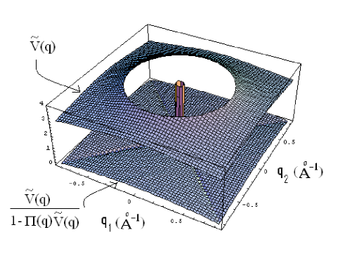
Figure 4: Plot of the screened and bare Coulomb contributions to the kernel of the Bethe-Salpeter equation, as functions of the wave vector $\mathbf{\widetilde{q}}$. Note the presence of an intense screening of the Coulomb repulsion in the considered here approximation.

Further, in the figure  4, the results of the evaluation of the screened Coulomb kernel of the bound state equation for two electrons (or two holes) are plotted, in common with the values of the bare kernel. Again the overlapping parameter and the Fermi energy are $\ a=0.95$ Å,  $\epsilon_{F}=-0.005\ eV$.    As it can be observed, in the considered approximation, the screening effect is noticeable.   Considering that the bare Coulomb interaction produces a repulsive potential of few $eV$ at distances of the order of the lattice constant, it follows that the screening effect could reduce these values down to ones of the order 0.1 $eV$ .  But, at such small repulsion forces other mechanisms, such as super-exchange or strong phonon interactions  could then create the necessary binding forces for the pairs to form.

Finally it should be remarked that in order to approach the present discussion to the real situation in the superconductor materials, it seems necessary to derive a similar picture but in a self-consistent approach.  A concrete way for this program could proceed in the following steps: a) To formulate the general Coulomb interacting problem of the valence electrons but retaining the Coulomb interaction exactly. b) Attempt to derive the here discussed tight binding model as a kind of HF approximation of the exact theory. c) After that, to derive and solve the Bethe-Salpeter equation for bounded pairs,  which should be expected to end including the anti-ferromagnetic interactions of the $tj$-model as a possible bounding mechanism Zhang_Rice . The consideration of this program is in progress.

References

• (1) E. Dagotto, Rev. Mod. Phys. 66, 763 (1994).
• (2) D. J. Scalapino, Phys. Rep. 250, 329 (1995).
• (3) D. C. Johnston, Normal-State Magnetic Properties of Single-Layer Cuprate High-Temperature Superconductors and Related Materials, in Handbook of Magnetic Materials, Vol. 10, Ed. K. H. J. Buschow Elsevier Science, Holland, 1997.
• (4) L. F. Mattheiss, Phys. Rev. Lett. 58, 1028 (1987).
• (5) W. Hanke and L. J. Sham, Phys. Rev. Lett. 33, 582 (1974).
• (6) W. Hanke and L. J. Sham, Phys. Rev. B 12, 4501 (1975).
• (7) O. Dolgov in: The Dielectric function of condensed systems, Eds.: L.V. Keldysh and D.A. Kirzhnitz and A.A. Maradudin (North-Holland, Amsterdam 1989).
• (8) D. C. Mattis, Coulomb Potencial in Layered Metals, Bloch States, Wannier Functions and High-Tc Superconductivity, Preprint UT 84112, Department of Physics, University of Utah, Salt Lake City, USA.
• (9) H. B. Schuttler, C. Grober, H. G. Evertz and W. Hanke,  Phys. Rev. E 64, 195105 (2001).
• (10) H.B. Schuttler, C. Grober, H. G. Evertz, and W. Hanke,  Overscreening in Hubbard electron systems,  arXiv:cond-mat/9805133, (1998).
• (11) J. van den Brink and G. A. Sawatzky, Eur. Phys. Lett. 50, 447 (2000).
• (12) V. I. Belyavsky and Yu. V. Kopaev, Phys. Rev. B 67, 024513 (2003).
• (13) M. Capezzali, D. Ariosa and H.Beck, Screening effects in superconductors, arXiv:cond-mat/9608119 (1996).
• (14) H. Shimahara, Effects of Short-Range Correlations on the Coulomb Screening and the Pairing Interactions in Electron-Phonon Systems: Triplet Pairing Mediated by Phonons, arXiv:cond-mat/0403628 (2004).
• (15) E. Koch, O. Gunnarsson, and R. M. Martin, Phys. Rev. Lett. 83, 620 (1999).
• (16) D. Pines, Elementary excitations in solids, (Benjamin, Ne York, 1964).
• (17) F. C. Zhang and T. M. Rice, Phys. Rev. B 37, 3759 (1988).
• (18) G. Wannier, JMP 19, 131 (1978).
• (19) G. Alecu, Rom. Rep. Phys. 56, 404 (2004).
• (20) C. Kittel, Introducción a la Física del Estado Sólido, (Reverté, Barcelona, 1993).
• (21) N. W. Ashcroft and N. D. Mermin, Solid State Physics, Ed. D.G. Crane (Holt, Rinehart and Winston, USA, 1976).
• (22) A. Fetter, A. L. and J. D. Walecka, Quantum Theory of Many-Particle Systems, (McGraw-Hill, New York, 1971).
• (23) S. Lundquist and N. H. March, Theory of the inhomogeneous electron gas, (Plenum Press, NewYork, 1983).