Macroscopic quantum tunnelling of Bose-Einstein condensates in a finite potential well

Abstract

Bose-Einstein condensates are studied in a potential of finite depth which supports both bound and quasi-bound states. This potential, which is harmonic for small radii and decays as a Gaussian for large radii, models experimentally relevant optical traps. The nonlinearity, which is proportional to both the number of atoms and the interaction strength, can transform bound states into quasi-bound ones. The latter have a finite lifetime due to tunnelling through the barriers at the borders of the well. We predict the lifetime and stability properties for repulsive and attractive condensates in one, two, and three dimensions, for both the ground state and excited soliton and vortex states. We show, via a combination of the variational and WKB approximations, that macroscopic quantum tunnelling in such systems can be observed on time scales of 10 milliseconds to 10 seconds.

1 Introduction

The tunnelling of a particle through a potential barrier is a fundamental effect in quantum mechanics [1]. Macroscopic quantum tunnelling is the tunnelling of a many-body wavefunction through a potential barrier, and therefore provides a more stringent test of the validity of quantum mechanics than the one particle case [2]. One place where the study of macroscopic quantum tunnelling is particularly experimentally accessible is in the tunnelling of a Bose-Einstein condensate (BEC) out of an optical trap. Recently, we showed that optical traps, which are of finite depth, can support both bound and quasi-bound states, and that the nonlinearity of the BEC mean field can be used to tune between them [3, 4, 5]. In this article, we calculate the lifetime of such quasi-bound states for both the ground state and excited soliton and vortex states. This provides a straightforward experimental observable for the occurrence of macroscopic quantum tunnelling of a BEC.

BEC’s exhibit different kinds of tunnelling phenomena. We consider the most direct generalization of the single-particle case [1], the tunnelling of the mean field through a barrier via the Gross-Pitaevskii, or nonlinear Schrödinger equation (NLS) [6]. We emphasize that this is a nonlinear tunnelling problem in the mean-field approximation [7]. Experimentally, tunnelling of the mean field in a double-well [8, 9] or sinusoidal lattice potential [10] in configuration space, as well as in spin space for multiple-spin-component BEC’s [11], has been investigated. There have been various theoretical studies related to these experiments [12, 13, 14, 15, 16, 17, 18, 19]. This is to be contrasted with tunnelling of the whole condensate in a variational parameter space, as was previously considered in the context of the collapse of a metastable attractive BEC in three dimensions [20, 21, 22, 23, 24] and in quantum evaporation of a bright soliton in an expulsive harmonic trap [7].

In this work, we consider a spherically symmetric trap in the form of a parabolic potential times a Gaussian, where the width of the Gaussian envelope is much greater than the harmonic oscillator length. This models the optical trap used in many experiments on BEC’s (see, for instance, [25]). A potential offset $V_{0}$ at the origin, which is important [3] in preventing collapse of attractive condensates in three dimensions [26], can be added with an additional blue- or red-detuned laser beam focused at the center of the trap. We take advantage of semi-classical methods and employ a variational-WKB formalism to calculate the lifetime of the condensate held in such a potential [7]. In addition, we calculate three critical values of the nonlinearity which could be observed in experiments: the point at which the condensate collapses, termed the collapse nonlinearity; the point at which the quasi-bound states are transformed into bound states, called the critical nonlinearity; and the point at which the condensate is pushed out over the top of the potential and quasi-bound states cease to exist at all, called the maximum nonlinearity. The collapse nonlinearity is observable as the point where the condensate first implodes. The critical nonlinearity is observable as the point where the lifetime first becomes longer than inverse experimental loss rates. The maximum nonlinearity is observable as the point where the condensate commences to expand.

We emphasize that even at the level of the mean field approximation, there are features that are distinctly different from the tunnelling of a single particle. As the tunnelling rate depends on the number of atoms remaining in the well, the lifetime is not simply inversely proportional to the rate as in the linear Schrödinger equation, but must be determined by an integral over each step of the tunnelling. The final state of the tunnelling process need not be that of zero probability of there being an atom remaining in the well. Instead, a quasi-bound repulsive condensate can decay towards a final bound state in which a finite number of atoms remain in the well. A quasi-bound attractive condensate can decay towards an unbound state so that the atoms spill out over the top of the well.

In Sec. 2, our application of the variational-WKB method to this nonlinear tunnelling problem is explained in detail. In Sec. 3 the lifetime and the three above-mentioned critical points are studied for the ground state in one, two, and three dimensions. Excited states are treated in Sec. 4.1 in one dimension for dark solitons and bright twisted solitons, and in Sec. 4.2 for vortices in two dimensions. In all cases we consider both repulsive and attractive condensates.

2 Fundamental equations and methods

The time-independent isotropic NLS with an external potential of the form described in Sec. 1 may be written as

$$-\frac{\hbar^{2}}{2M}\nabla^{2}\tilde{\Psi}+\tilde{V}(\tilde{r})\tilde{\Psi}+\tilde{U}_{D}|\tilde{\Psi}|^{2}\tilde{\Psi}=\tilde{\mu}\tilde{\Psi}\,,$$ (1)

$$\tilde{V}(\tilde{r})=\left(\tilde{V}_{0}+\frac{1}{2}M\omega^{2}\tilde{r}^{2}\right)\exp\left(-\tilde{r}^{2}/2\ell_{\mathrm{Gauss}}^{2}\right)\,,$$ (2)

$$\beta_{D}\int_{0}^{\infty}d\tilde{r}\,\tilde{r}^{D-1}|\tilde{\Psi}|^{2}=1\,,$$ (3)

where the tildes indicate that the respective variables and parameters are measured in physical units. Here $\tilde{\Psi}$ is the mean-field wavefunction with the integral norm set to unity, $M$ is the atomic mass, $\tilde{\mu}$ is a complex eigenvalue which we term the chemical potential, $\ell_{\mathrm{Gauss}}$ is the width of the Gaussian envelope, $\omega$ is the angular frequency of the parabolic trap, and $\tilde{V}_{0}$ is the potential offset at the origin. The constant

$$\beta_{1,2,3}\equiv 2,2\pi,4\pi$$ (4)

for the spatial dimension $D=1,2,3$. The coupling constants are renormalized appropriately for the dimensionality:

$$\tilde{U}_{1,2,3}=(2\hbar\omega_{\perp})aN\,,\,\left(\sqrt{\frac{8\pi\hbar^{3}\omega_{z}}{M}}\right)\,aN\,,\,\left(\frac{4\pi\hbar^{2}}{M}\right)aN\,\,,$$ (5)

where $a$ is the $s$-wave scattering length and $N$ is the number of atoms. The transverse oscillator frequencies $\omega_{\perp},\omega_{z}$ must be sufficiently high so as to reduce the effective dimensionality of the mean field of the BEC [27, 28, 29, 30].

The NLS can be conveniently rescaled to dimensionless form:

$$-\frac{1}{2}\nabla^{2}\Psi+V(r)\Psi+U_{D}|\Psi|^{2}\Psi=\mu\Psi\,,$$ (6)

$$V(r)=\left(V_{0}+\frac{1}{2}r^{2}\right)\exp\left(-\alpha\,r^{2}\right)\,,$$ (7)

$$\beta_{D}\int_{0}^{\infty}dr\,r^{D-1}|\Psi|^{2}=1\,,$$ (8)

where all variables are in units of the harmonic oscillator energy $\hbar\omega$ and length $\ell_{\mathrm{ho}}\equiv\sqrt{\hbar/m\omega}$. The coupling constants become

$$U_{1,2,3}=aN/\ell_{{\mathrm{ho}}}\,,\sqrt{2/\pi}\,aN/\ell_{{\mathrm{ho}}}\,,aN/\ell_{{\mathrm{ho}}}\,.$$ (9)

The parameters $V_{0}$ and

$$\alpha\equiv(\ell_{\mathrm{ho}}/\ell_{\mathrm{Gauss}})^{2}$$ (10)

characterize the structure of the potential. For a broad Gaussian envelope, which pertains to the experimentally available optical trap described in Sec. 1, $\alpha\ll 1$.

Approximate solutions to Eq. (6) with potential (7) can be obtained via the variational method. The ansatz we use in each of the cases to be considered below contains a Gaussian factor of form $A\,\exp[-r^{2}/(2\rho^{2})]$, with the amplitude $A$ and the width $\rho$ taken as variational parameters. Substituting the ansatz into the normalization condition (8) and the Lagrangian of the NLS (for the time being, $\mathrm{Im}(\mu)$ is disregarded), one minimizes the Lagrangian with respect to $\rho$ and $A$. Then one obtains a system of equations for the nonlinearity $U_{D}$ and the real part of the chemical potential $\mathrm{Re}(\mu)$ in terms of given parameters of the system, $D$, $\alpha$, and $V_{0}$. The solution is stable in the framework of the time-dependent radially symmetric NLS if

$$d\mathrm{Re}(\mu)/d|U_{D}|\leq 0\,,$$ (11)

which is known as the Vakhitov-Kolokolov (VK) criterion [31]. An important point is that our choice of ansatz truncates the solution space by requiring the wavefunction decay as $r\rightarrow\infty$, eventually enabling us to find quasi-bound states in the form of eigenstates with complex eigenvalues.

To find the imaginary part of the chemical potential one can separately apply the WKB approximation [1, 32]. The tunnelling rate $\gamma$ in $D$ dimensions is given by the standard expressions

$$\gamma = \nu\,\exp\left(-2\int_{r_{1}}^{r_{2}}dr\,|p(r)|\right)\,,$$ (12)

$$p(r) \equiv \sqrt{2[\mu-V_{D}^{\mathrm{eff}}(r)]}\,,$$ (13)

$$\nu^{-1} \equiv 4\int_{0}^{r_{1}}\frac{dr}{|p(r)|}\,,$$ (14)

where the endpoints $r=r_{1}$ and $r=r_{2}$ are found from setting the semiclassical momentum $p(r)=0$ and

$$V_{1}^{\mathrm{eff}}(r) \equiv V(r)+U_{1}|\phi_{1}|^{2}\,,$$ (15)

$$V_{2}^{\mathrm{eff}}(r) \equiv V(r)-\frac{1}{8r^{2}}+\frac{U_{2}}{r}|\phi_{2}|^{2}\,,$$ (16)

$$V_{3}^{\mathrm{eff}}(r) \equiv V(r)+\frac{U_{3}}{r^{2}}|\phi_{3}|^{2}\,.$$ (17)

Here $\nu$ is the semiclassical oscillation frequency in the well. The imaginary part of the chemical potential is then given by

$$\mathrm{Im}(\mu)=-\gamma/2\,.$$ (18)

Note that $\gamma$ must be multiplied by $2$ in the 1D case, to account for tunnelling from both sides of the well. The transformed wavefunctions in Eqs. (15)-(17) are given by the standard expressions

$$\phi_{1,2,3}=\Psi\,,\,\sqrt{r}\Psi\,,\,r\Psi\,.$$ (19)

In the case of axially symmetric excited states in 2D, i.e., vortices, it is useful to make the phase winding number explicit:

$$\phi_{2}=\phi_{2,m}e^{im\theta}\,.$$ (20)

Then the transformed wavefunction $\phi_{2,m}$ leads to the simplified NLS

$$-\frac{1}{2}\frac{\partial^{2}}{\partial r^{2}}\phi_{2,m}+V_{2,m}^{eff}\phi_{2,m}=\mu\,\phi_{2,m}\,,$$ (21)

where the effective potential is

$$V_{2,m}^{eff}=V(r)+\frac{m^{2}-1/4}{2\,r^{2}}+\frac{U_{2}}{r}|\phi_{2,m}|^{2}\,.$$ (22)

Note that the centrifugal barrier changes sign for $m\neq 0$, so that the semiclassical period of oscillation in the well must be redefined as

$$\nu^{-1}=2\int_{r_{0}}^{r_{1}}\frac{dr}{|p(r)|}\,,$$ (23)

where $r_{0}$ is the inner turning point created by the centrifugal barrier. The outer potential barrier is delimited by $r_{1},\,r_{2}$.

The main experimental observable we consider is the lifetime of the trapped condensate. This is not given by $1/\gamma$, as in a linear system, but must be found from the rate equation

$$dN/dt=-\gamma(N)N\,,$$ (24)

where $\gamma(N)$ is the nonlinear tunnelling rate and $N$ is the number of atoms in the BEC remaining in the trap, i.e., between the classical turning points. This leads to the integral

$$T=\int_{N_{0}}^{N_{0}/e}dN/[-\gamma(N)N]\,,$$ (25)

where $T$ is the lifetime and $N_{0}$ is the initial number of atoms in the well. Here we have assumed that the atomic interaction strength $a$ and the harmonic oscillator length $\ell_{\mathrm{ho}}$ are constant in time. Therefore, in practice, we integrate over the norm $U_{D}$, which is proportional to $N$.

Besides the lifetime, there are three important quantities we will calculate. The maximum nonlinearity $U_{D}^{\mathrm{max}}$ is the point at which the condensate spills out over the top of the well and a quasi-bound state ceases to exist. The critical nonlinearity $U_{D}^{\mathrm{crit}}$ is the point at which the real part of the chemical potential changes from positive to negative, the imaginary part goes to zero, and the quasi-bound state is transformed into a genuine bound state. The collapse nonlinearity $U_{D}^{\mathrm{coll}}$ is the point at which the condensate collapses in two and three dimensions, as we will explain in more detail in the following section.

There is an important subtlety in the limits of integration in Eq. (25). We can define an $N^{\mathrm{crit}}\propto U_{D}^{\mathrm{crit}}$ and $N^{\mathrm{max}}\propto U_{D}^{\mathrm{max}}$. If $U_{D}^{\mathrm{crit}}>0$, then the nonlinearity is always repulsive for tunnelling processes. The upper limit of Eq. (25) must be replaced with $(N_{0}-N_{\mathrm{crit}})/e+N_{\mathrm{crit}}$, and we define the lifetime with respect to decay to a stable state. That is to say, no more than $(N_{0}-N_{\mathrm{crit}})$ particles will ever leave the well. On the other hand, if $U_{D}^{\mathrm{max}}<0$, then the nonlinearity is always attractive. The upper limit of Eq. (25) must then be replaced with $(N_{0}-N_{\mathrm{max}})/e+N_{\mathrm{max}}$, and we define the lifetime with respect to decay to a non-stationary state. In this case, after $(N_{0}-N_{\mathrm{max}})/e$ particles have left the well via quantum mechanical tunnelling, the rest simply flow over the top classically. These cases are extremely different from tunnelling of a single atom in the linear Schrödinger equation, where the final state always corresponds to zero atoms remaining in the well.

3 Tunnelling of the Ground State in One, Two, and Three Dimensions

Taking the variational ansatz as a Gaussian,

$$\Psi_{\mathrm{gs}}=A\,\exp\left(-\frac{r^{2}}{2\rho^{2}}\right)\,,$$ (26)

one minimizes the Lagrangian corresponding to Eq. (6). The result is a system of Euler-Lagrange equations for the chemical potential and nonlinearity [33, 34]. These take the form

$$\mathrm{Re}(\mu) = \frac{1}{4}\left\{(-4+D)\rho^{-2}+(1+\alpha\rho^{2})^{-2-D/2}\right.$$ (27)

$$\left.\times\left[4V_{0}+(4+D)\rho^{2}\right.\left.-\alpha(D+4V_{0}\alpha)\rho^{4}\right]\right\}\,,\,\,\,\,\,\,$$

$$U_{D} = \Gamma(D/2)2^{-2+D/2}\beta\rho^{-2+D}(1+\alpha\rho^{2})^{-2-D/2}$$ (28)

$$\times\left\{-2(1+\alpha\rho^{2})^{2+D/2}+\rho^{4}[2-4V_{0}\alpha-\alpha(D+4V_{0}\alpha)\rho^{2}]\right\},::::::$$

where $\Gamma(D/2)$ is a Gamma function and $D$ is the dimensionality.

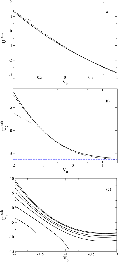
Figure 1: Ground state transition. Shown is the critical nonlinearity for a transition from a bound to a quasi-bound state, as a function of the potential offset $V_{0}$. (a) One dimension, $\alpha=1,1/2,1/10$ (dotted, dashed, solid curves), where $\alpha\equiv\ell_{\mathrm{ho}}^{2}/\ell_{\mathrm{Gauss}}^{2}$. There is no collapse in one dimension. (b) Two dimensions: $\alpha=1,1/2,1/10$ (dotted, dot-dashed, solid curves); the critical nonlinearity for collapse, $U_{2}^{\mathrm{coll}}=-2\pi$ is indicated by the blue dashed curve. Note that the condition $U_{2}^{\mathrm{crit}}>U_{2}^{\mathrm{coll}}$ always holds. (c) Three dimensions: $\alpha=1,1/2,1/3,1/4,1/5,1/6,1/7$ from bottom left to top right. The collapse point is described in Fig. 2.

The transition from a quasi-bound to a bound state occurs when the real part of the chemical potential changes sign from positive to negative, since our potential $V(r)\rightarrow 0^{+}$ as $r\rightarrow\infty$. The nonlinearity at which this occurs we termed $U_{D}^{\mathrm{crit}}$. In Fig. 1 is shown the dependence of $U_{D}^{\mathrm{crit}}$ on the potential offset $V_{0}$, as defined in Eq. (7). The cases of $D=1,2,3$ dimensions are illustrated in separate panels in the figure. The different curves in each panel pertain to different values of the trap-shape parameter $\alpha$. These two continuous parameters, $V_{0}$ and $\alpha$, and the discrete one, $D$, are the only given constants in the system. The potential offset $V_{0}$ can be controlled by a red- or blue-detuned laser focused at the center of the trap, as previously mentioned.

However, the existence of the transition from a quasi-bound to a bound state does not mean that the ground state solution we obtained is stable. When the nonlinearity is negative, so that the atoms attract each other, the condensate can collapse. In three dimensions with $V(r)=0$, any initial condition leads to collapse [26]. As is well-known for BEC’s, the imposition of a nonzero potential $V(r)$ can create a metastable solution with a lifetime much longer than that of the BEC, so that it is experimentally stable. This requires a nonlinearity which is not too strongly negative, $U_{3}>U_{3}^{\mathrm{coll}}$, where $U_{3}^{\mathrm{coll}}$ is the critical point for collapse. This critical point can be determined variationally or numerically [35, 36, 3]. In order to observe the transition from a quasi-bound to a bound state, it is necessary that $U_{3}^{\mathrm{coll}}<U_{3}^{\mathrm{crit}}$, as we showed recently [3]. The critical nonlinearity for collapse corresponds to an eigenvalue $\mu^{\mathrm{coll}}$, while $U_{3}^{\mathrm{crit}}$ corresponds to $\mu=0$. Therefore a simple way to state this condition is

$$\mu^{\mathrm{coll}}<0\,.$$ (29)

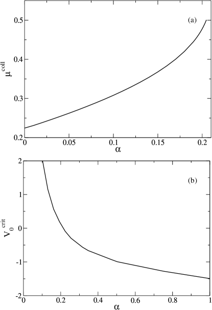
Figure 2: Ground state parameters, three dimensions. (a) Shown is the dependence of the collapse point on the trap-shape parameter $\alpha$ for zero offset ($V_{0}=0$). For nonzero $V_{0}$ and $\alpha\ll 1$, $\mu^{\mathrm{coll}}\simeq\mu^{\mathrm{coll}}(V_{0}=0)+V_{0}$. In order to obtain an observable transition from a quasi-bound to a bound state, it is necessary that $\mu^{\mathrm{coll}}<0$. (b) Shown is the critical offset $V_{0}^{\mathrm{crit}}$ needed to obtain any quasi-bound state for a given $\alpha$: $V_{0}\leq V_{0}^{\mathrm{max}}$.

In Fig. 2(a), $\mu^{\mathrm{coll}}$ is shown as a function of the trap parameter $\alpha$ for $V_{0}=0$. Clearly, in order to observe the transition from a quasi-bound to a bound state in three dimensions, one needs a finite offset $V_{0}<0$, as was shown in Ref. [3]. For $\alpha\ll 1$, the effect of a nonzero offset $V_{0}$ on $\mu^{\mathrm{coll}}$ is essentially linear: $\mu^{\mathrm{coll}}\simeq\mu^{\mathrm{coll}}(V_{0}=0)+V_{0}$. For instance, to observe the transition from the quasi-bound state to the bound one, it is required that $V_{0}\leq-0.273$ for $\alpha=1/4$. For larger $\alpha$, the relation between $\mu$ and $V_{0}$ becomes nonlinear. For example, in the case of $\alpha=1$, the necessary condition is $V_{0}\leq-1.495$. Since such values of $\alpha$ are experimentally irrelevant, we do not illustrate this regime.

Inspection of Fig. 2(a) reveals that the curve terminates at $\alpha=0.2$. For $\alpha>0.2$ and $V_{0}=0$, there is no quasi-bound state at all. Another way of stating this is that for any $\alpha$, there is a critical $V_{0}^{\mathrm{crit}}$ such that

$$V_{0}\leq V_{0}^{\mathrm{crit}}$$ (30)

is required to obtain any stationary solution of the form described by the ansatz of Eq. (26). A plot expressing this condition is displayed in Fig. 2(b). This is an important consideration in choosing the correct experimental regime to observe quasi-bound states in three dimensions.

In 1D there is no collapse at all. In 2D and in free space, initial conditions lead to collapse for $U_{2}<U_{2}^{\mathrm{coll}}$ and expansion for $U_{2}>U_{2}^{\mathrm{coll}}$, while for $U_{2}=U_{2}^{\mathrm{coll}}$ an unstable stationary state is obtained, known as the Townes soliton [26]. This weak collapse is different from the strong collapse which occurs in 3D [26]. An appropriate external potential can stabilize the expanding regime, producing a stable solution, rather than a metastable one as in 3D (see, for instance, the discussion in Ref. [40]). The value $U_{2}^{\mathrm{coll}}$ which determines the collapse threshold can be derived from Eqs. (27)-(28) by taking $\rho\rightarrow 0^{+}$. Then $\mu\rightarrow-\infty$ and

$$U_{2}^{\mathrm{coll}}=-2\pi\,.$$ (31)

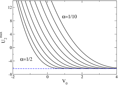
Figure 3: Ground state parameters, two dimensions. (a) Shown is the dependence of the maximum nonlinearity $U_{2}^{\mathrm{max}}$ to obtain a quasi-bound state on the potential offset $V_{0}$. The curves show $\alpha=1/2,1/3,\ldots,1/10$ from bottom left to top right. The dashed blue line shows the collapse point, $U_{2}^{\mathrm{coll}}=-2\pi$. In this harmonic times Gaussian potential, one is therefore limited to the range of nonlinearities $U_{2}^{\mathrm{coll}}<U_{2}<U_{2}^{\mathrm{max}}$. Note that for $U_{2}\leq U_{2}^{\mathrm{coll}}$ there is no stationary state at all.

A third critical nonlinearity is given by the point at which the eigenvalue $\mu=\max[V(r)]$, i.e., where the quasi-bound state ceases to exist. We called this maximum nonlinearity $U_{2}^{\mathrm{max}}$. The range of allowed nonlinearities for obtaining a stationary state is therefore given by $U_{2}^{\mathrm{coll}}<U_{2}<U_{2}^{\mathrm{max}}$. In this range all solutions are stable or quasi-stable. Outside of this range there are no stationary states. Figure 3 illustrates the dependence of $U_{2}^{\mathrm{max}}$ on the other parameters in the problem. The collapse point is shown as a dashed blue line. Note that the inequalities $U_{2}^{\mathrm{coll}}<U_{2}^{\mathrm{crit}}<U_{2}^{\mathrm{max}}$ hold for all shapes of the trap, unlike the 3D case.

A technical point concerning two dimensions is that there is always an additional solution with large $\rho$ which is radially unstable within the context of our Gaussian ansatz and the VK criterion. This corresponds to a ring of condensate around the trap. Its variational form and stability can be more appropriately investigated with a vortex-like ansatz, as we briefly discuss in Sec. 4.2.

A clear experimental signature for a quasi-bound to bound state transition is a change in the lifetime of the condensate. Suppose that the lifetime due to tunnelling of the wave function is on the order of or much less than that imposed by three body processes, scattering with the background gas in the vacuum, and other sources of loss. One can then determine the difference between a quasi-bound and bound state by measuring the number of atoms in the trap as a function of time. It is necessary to choose the right experimental parameters in order to have a realistically observable lifetime. For instance, typical BEC lifetimes are on the order of ten to a hundred seconds. However, the mean-field induced dynamical time scales are typically on the order of milliseconds. Therefore, a lifetime due to tunnelling on the order of 10 milliseconds to 1 second is desirable.

In Fig. 4 we show the lifetime for several values of $\alpha$. Panels (a)-(c) pertain to one, two, and three dimensions. The lifetime is calculated from Eq. (25), as discussed in Sec. 2. The leftmost endpoint of the curves corresponds to $U_{D}^{\mathrm{crit}}$. When $U_{D}^{\mathrm{crit}}>0$ the final state is bound and has a nonzero number of atoms. Three examples are shown for $D=3$ in Fig. 4(c). The rightmost endpoint of the curves corresponds to $U_{D}^{\mathrm{max}}$. When $U_{D}^{\mathrm{max}}<0$, the final state is unbound and the remaining atoms spill out over the top of the trap without tunnelling. Two examples are shown for $D=2$ in Fig. 4(b).

Since the lifetime is scaled to the trap frequency $\omega$, one can convert the range of $T$ to milliseconds easily. For instance, for a trap of angular frequency $\omega=2\pi\times 100$ Hz, the range $T=10$ to $10^{4}$ shown in Fig. 4 corresponds to 16 ms to 16 s. Thus the trap parameters chosen for the figure result in experimentally observable lifetimes.

The relationship between the tunnelling rate, defined by Eq. (12), and the lifetime, defined by Eq. (25), can be very non-intuitive with respect to what is known from single-particle tunnelling in the linear Schrödinger equation. For example, in Fig. 4(c) the lifetime approaches zero on the left hand side as $U_{3}\rightarrow U_{3}^{\mathrm{crit}}>0$. This can be physically understood in terms of the tunnelling of the wavefunction through the effective potential. As the real part of the chemical potential approaches zero from above, so that the quasi-bound state becomes a bound state, the attractive nonlinearity pulls down the potential barrier. That is, the effective potential barrier shrinks. In the case of three dimensions, and for $\mathrm{Re}(\mu)<0$, it is well-known that the attractive nonlinearity can dominate over both the kinetic energy and the potential energy, leading to strong self-focusing and collapse. Here, one observes that the attractive nonlinearity already dominates over the potential energy barrier for $\mathrm{Re}(\mu)>0$. This causes the effective potential barrier to disappear for a very narrow region of $U_{3}$ near the formation of the bound state, so that the lifetime goes to zero. This region is so narrow that it is not experimentally relevant, since number fluctuations cannot be finely controlled in BEC experiments, and $U_{3}\propto N$.

One can more rigorously understand the limiting values of the lifetime in the form of the power law of the tunnelling rate $\gamma$ as $U_{3}\rightarrow\left(U_{3}^{\mathrm{crit}}\right)^{+}$. Suppose the power law takes the form

$$\gamma(U_{D})\simeq\left(U_{D}-U_{D}^{\mathrm{final}}\right)^{p}\,,$$ (32)

where $p$ is a real positive constant and $U_{D}^{\mathrm{final}}$ can be zero, $U_{D}^{\mathrm{max}}$, or $U_{D}^{\mathrm{crit}}$, depending on the allowed domain of quasi-bound states (see the discussion of the appropriate integration limits following Eq. (25)). By expanding the integral according to $\int_{a}^{a+\epsilon}dx\,f(x)\simeq\epsilon f(a)$, one finds that for $0\leq p<1$ the lifetime approaches zero, despite the rate approaching zero. For $p>1$ the lifetime approaches infinity, while for $p=1$ it approaches a nonzero constant. We find numerically for the ground state that whenever $U_{D}^{\mathrm{final}}=U_{D}^{\mathrm{crit}}>0$ or $U_{D}^{\mathrm{final}}=U_{D}^{\mathrm{max}}<0$ the power law of the rate is such that the lifetime approaches zero at these critical points. For $U_{D}^{\mathrm{final}}=0$, which occurs when $U_{D}^{\mathrm{crit}}<0$ and $U_{D}^{\mathrm{max}}>0$, $p=1$ and the lifetime approaches a nonzero constant.

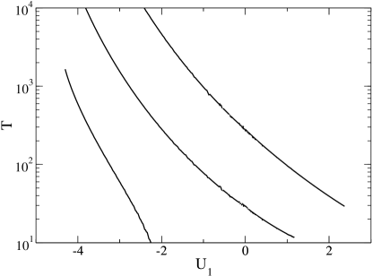
Figure 6: Excited state lifetime, soliton. Shown is the lifetime of the excited state with a single node in one dimension, i.e., a dark soliton for $U_{1}>0$ and a bright twisted soliton for $U_{1}<0$. The parameters are $V_{0}=0$ and $\alpha=1/6,1/8,1/10$ from left to right.

Finally, we note one other important point about the lifetime. For $U_{D}=0$, where there is no mean field, one recovers the correct single-particle $T=1/\gamma$, as can also be seen by consideration of Eq. (25). This is a limiting case in the center of a smooth lifetime curve in Fig. 4 (see also Figs. 6 and 9 below). Therefore, it strongly supports the validity of the mean field approximation.

4 Tunnelling of Excited States

4.1 Soliton Tunnelling in One Dimension

The variational ansatz

$$\Psi_{\mathrm{sol}}=A\,r\exp\left(-\frac{r^{2}}{2\rho^{2}}\right)$$ (33)

models the excited state with a single node in one dimension. This is a dark soliton for $U_{1}>0$, i.e., a repulsive BEC in 1D, and an antisymmetric, or bright twisted soliton for $U_{1}<0$, i.e., an attractive BEC in 1D. The variational equations for the chemical potential and nonlinearity may be derived by means of the methods outlined in Sec. 2:

$$\mathrm{Re}(\mu) = \frac{1}{4}\left\{-9\rho^{-2}+(1+\alpha\rho^{2})^{-7/2}\left[4V_{0}+(15-16V_{0}\alpha)\rho^{2}\right.\right.$$ (34)

$$\left.\left.-5\alpha(3+4V_{0}\alpha)\rho^{4}\right]\right\}\,,\,\,\,\,\,\,$$

$$U_{1} = \frac{2\sqrt{2\pi}}{\rho}\left\{-2+(1+\alpha\rho^{2})^{-7/2}\rho^{4}\left[2-4V_{0}\alpha\right.\right.$$ (35)

$$\left.\left.-\alpha(3+4V_{0}\alpha)\rho^{2}\right]\right\}\,,$$

A plot of $U_{1}^{\mathrm{crit}}$, the dependence of the critical nonlinearity for the transition from a quasi-bound state to a bound state, is shown in Fig. 5. The transition point is only very weakly dependent on $\alpha$ for $\alpha\ll 1$. This regime is an experimental relevant one.

Figure 6 shows the main experimental observable characteristic of quasi-bound solitons, namely, the lifetime. The node causes the wavefunction to become somewhat broader than the ground state. This requires smaller values of $\alpha$ in order to provide sufficiently thick walls to hold the quasi-bound condensate, in comparison to Fig. 4(a). As was true for the ground state, the leftmost endpoint of the curves corresponds to $U_{1}^{\mathrm{crit}}$, while the rightmost endpoint corresponds to $U_{1}^{\mathrm{max}}$. For $\alpha=1/6$ and $V_{0}=0$, one finds $U_{1}^{\mathrm{max}}<0$. Thus, after losing some atoms via tunnelling through the barrier, the final state takes the form of two bright solitons with a phase difference of $\pi$ which travel in opposite directions away from the potential center.

4.2 Vortex Tunnelling in Two Dimensions

Under the assumption of an axisymmetric stationary state in two dimensions, one may take the variational ansatz for a vortex state as

$$\phi_{m}^{\mathrm{vor}}=A\,r^{m}\exp\left(-\frac{r^{2}}{2\rho^{2}}\right)\exp(im\theta)\,,$$ (36)

where $m$ is the winding number, or topological charge. Then, transforming the ansatz according to Eq. (20) and minimizing the Lagrangian with respect to Eq. (21) with effective potential (22), one derives the following system of equations for the chemical potential:

$$\mathrm{Re}(\mu) = \frac{1}{2\,\Gamma(1+m)}\left\{-\frac{\Gamma(2+m)}{\rho^{2}}+(1+\alpha\rho^{2})^{-3-m}\right.$$ (37)

$$\left.\times\left[-2V_{0}(1+\alpha\rho^{2})(-1+(1+2m)\alpha\rho^{2})\Gamma(1+m)\right.\right.$$

$$\left.\left.-\rho^{2}(-3+(1+2m)\alpha\rho^{2})\Gamma(2+m)\right]\right\}\,,\,\,\,\,\,\,$$

$$U_{2} = -\frac{\Gamma(1+m)\Gamma(2+m)\,2^{1+2m}\pi}{\Gamma(1+2m)}\left\{1+(1+\alpha\rho^{2})^{-3-m}\right.$$ (38)

$$\left.\times\rho^{4}\left[-1+2V_{0}\alpha+\alpha(1+m+2V_{0}\alpha)\rho^{2}\right]\right\}\,,$$

As a consistency check, note that, for the case $m=0$, one recovers the same result as given by Eqs. (27) and (28) with $D=2$.

The collapse point may be obtained by expansion of Eqs. (37) and (38) in small $\rho$, in the same way as was done in Sec. 3. One thus finds

$$U_{2}^{\mathrm{coll}}=-\frac{2\pi^{3/2}\Gamma(2+m)}{\Gamma(1/2+m)}\,.$$ (39)

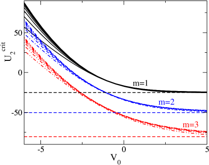
Figure 7: (color online) Excited state transition, vortex. The critical nonlinearity for a transition from a quasibound to a bound state is shown, in analogy to Fig. 3(b), for values of the winding number $m=1$ (solid black curves), $m=2$ (dot-dashed blue curves), and $m=3$ (dot-dot-dashed red curves). Each set of curves rises along the $y$-intercept for decreasing $\alpha$ as $\alpha=3^{-2},\,4^{-2},\,\ldots,\,10^{-2}$. The dashed horizontal lines show the nonlinearities for which the solutions collapse: $U_{2}^{\mathrm{coll}}=-8\pi,-16\pi,-(128/5)\pi$ for $m=1,2,3$. Note that $U_{2}^{\mathrm{crit}}>U_{2}^{\mathrm{coll}}$ for all $V_{0},\alpha,m$.

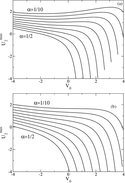
Figure 8: Excited state parameters, vortex. Shown is the dependence of the maximum nonlinearity for confinement of a vortex, $U_{2}^{\mathrm{max}}$, on the parameters $V_{0},\alpha,m$. Here $V_{0}$ is the potential offset, $\alpha$ the trap-shape parameter, and $m$ the vortex winding number. Panels (a) and (b) illustrate $m=1$ and $2$, respectively, while $\alpha=1/2,1/3,\ldots,1/10$ from bottom to top in each panel. The asymptotic right hand value of each curve represents the critical parameter set for which a vortex is pushed outside the potential, i.e., where it becomes pinned rather than confined.

For $m=0,1,2,3$ one obtains $U_{2}^{\mathrm{coll}}=-2\pi,\,-8\pi,\,-16\pi,\,-(128/5)\pi$. The presence of the vortex decreases the collapse point, as was pointed out some time ago [35, 37, 38]. The critical point for a transition from a quasi-bound to a bound state is shown in Fig. 7 for $m=1,2,3$. Like the ground state in two dimensions, the nonlinearity is constrained to the range $U_{2}^{\mathrm{coll}}<U_{2}<U_{2}^{\mathrm{max}}$. In Fig. 8 the allowed range is shown as a function of $\alpha$ and $V_{0}$ for $m=1,2$.

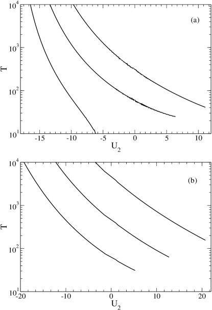
Figure 9: Excited state lifetime, vortex. Shown is the lifetime of the condensate with a vortex in two dimensions. (a) Winding number $m=1$ and trap-shape parameter $\alpha=1/8,\,1/10,\,1/12$. (b) $m=2$ and $\alpha=1/14,/,1/16,\,1/18$. The leftmost point of each curve, which is not shown on the plot, approaches $U_{2}^{\mathrm{crit}}$, where $\mu\rightarrow 0^{+}$, the quasi-bound state disappears, and the lifetime $T\rightarrow\infty$. The rightmost point corresponds to $U_{2}^{\mathrm{max}}$, where a quasi-bound state is no longer supported by the potential (see Fig. 8).

The lifetime of the condensate with a vortex is shown in Fig. 9 for $m=1,2$. For higher winding numbers the ansatz becomes broader, and it is necessary to choose smaller $\alpha$ in order to contain the vortex. This is reflected in the range of $\alpha$ in Fig. 9, $\alpha=1/8$ to $1/12$ for $m=1$ and $\alpha=1/14$ to $1/18$ for $m=2$. Note that, unlike for the cases illustrated in Figs. 4 and 6, here $T\rightarrow\infty$ as $U_{2}\rightarrow U_{2}^{\mathrm{crit}}$. In Fig. 9(a), for $\alpha=1/8$ the atoms first tunnel through the barrier. When $U_{2}$ reaches $U_{2}^{\mathrm{max}}<0$, the condensate spills out over the top of the potential barrier. Then it expands towards $r=\infty$ as a bright ring soliton [39, 40], pushed outwards by the Gaussian tail of the potential. At a critical value of the ring radius, it undergoes azimuthal modulational instability [41].

We have not considered azimuthal instabilities. These should be manifest for nonzero winding number in the attractive case in 2D in certain parameter regimes [39, 42]. A simple stability criterion is that the wavelength of modulational instability be longer than the ring circumference $2\pi\rho$ (for details, see [40] and references therein). A more sophisticated treatment via a full linear stability analysis (using the Bogoliubov equations) is left for a future work.

We note that for nonzero winding number there is an additional stationary state which has a radius greater than that of the potential peak. For repulsive nonlinearity, this is a radially unstable pinned vortex with an initial core size artificially controlled via the trapping potential. For attractive nonlinearity, this state can be radially stabilized for sufficiently strong nonlinearity, as may be shown via the VK criterion of Eq. (11). However, in this regime we expect the azimuthal instability to dominate, so we have not presented it here in any detail.

5 Conclusion

In this study we suggested a straightforward macroscopic quantum tunnelling experiment which requires little or no modification of existing experimental apparatus. We assumed a trap consisting of a parabolic potential times a Gaussian envelope, which models typical optical traps used in experiments. Such a trap supports both bound and quasi-bound states. Using a variational-WKB mean-field formalism, we calculated four experimental observables: the lifetime $T$ of quasi-bound condensates; the maximum nonlinearity $U_{D}^{\mathrm{max}}$ for which a quasi-bound state exists; the critical nonlinearity $U_{D}^{\mathrm{crit}}$ for which a quasi-bound state becomes a bound state; and, for two and three dimensions, the collapse nonlinearity $U_{D}^{\mathrm{coll}}<0$.

By adjusting the initial number of atoms and/or the atomic interaction strength, as may be achieved via a Feshbach resonance [vogels1997, 44, 45], we showed how a quasi-bound condensate can be adiabatically transformed into a bound one, and vice versa. We presented in detail the parameter regimes in which such a transformation can be performed for both repulsive and attractive condensates. In two dimensions, we found that the relations $U_{2}^{\mathrm{max}}>U_{2}^{\mathrm{crit}}>U_{2}^{\mathrm{coll}}$ always hold; in three dimensions, it is necessary to add a negative offset to the potential at $r=0$ in order to observe the quasi-bound to bound transition without provoking collapse of the condensate. This offset can be constructed with an off-resonant blue- or red-detuned laser focused at the origin of the trap.

We found that, for reasonable experimental parameters, one could observe the tunnelling of a BEC through the walls of an optical trap on time scales of 10 milliseconds to 10 seconds. We showed that tunnelling can lead to a final state which is quite different from that obtained via the linear Schrödinger equation. For $U_{D}^{\mathrm{crit}}>0$, an initially quasi-bound repulsive condensate approaches a bound state with a finite number of atoms remaining in the well. For $U_{D}^{\mathrm{max}}<0$ an initially quasi-bound attractive condensate approaches an unbound state for which the atoms spill out over the top of the well. This is observable as a pair of counter-propagating bright solitons in one dimension, and as an azimuthally unstable bright ring soliton in two dimensions [39, 40].

We showed previously that our variational-WKB method accurately determines the tunnelling rate and critical points at the level of 1% or better, except near the collapse points, where it is accurate to within about 10% [3]. It is also possible to test our method via exact solution with a small number of atoms. For example, it has been shown that mean field effects are strongly evident in as few as three bosons confined in an external potential [46].

Finally, we note that there is a direct analogy between the operation of a laser and the tunnelling of a BEC through the walls of an optical trap. In a laser operating well above threshold, the coherent state in the cavity is robust against removal of single photons via tunnelling through a thin barrier. This is the essence of a coherent state. The mean field of the Bose condensate in an optical trap is phase-coherent and robust in the same way. Therefore we expect our mean field approximation to be an excellent one for a large initial number of atoms in the trap. When the initial number of atoms becomes very small, the condensate is liable to phase fluctuations. However, as our lifetime definition and figures have the right single-particle limit for zero mean field, we expect that the mean field theory also gives good results in this region.

We acknowledge useful discussions with Yehuda Band, Nimrod Moiseyev, and Brian Seaman. L. D. Carr and M. J. Holland acknowledge the support of the U.S. Department of Energy, Office of Basic Energy Sciences via the Chemical Sciences, Geosciences and Biosciences Division. B. A. Malomed acknowledges support from the Israel Science Foundation, through grant No. 8006/03, and appreciates the hospitality of JILA (University of Colorado, Boulder).

Figure 4: Ground state lifetime. Shown is the lifetime $T$ of the BEC, scaled to the trap frequency $\omega$, for zero potential offset $V_{0}$ and for several values of the trap-shape parameter $\alpha\equiv\ell_{\mathrm{ho}}^{2}/\ell_{\mathrm{Gauss}}^{2}$, as a function of the initial nonlinearity $U_{D}\propto N$. (a) $D=1$, $V_{0}=0$, $\alpha=1/4,1/5,1/6,1/7,1/8$ (from bottom to top). (b) $D=2$, $V_{0}=0$, $\alpha=1/4,1/5,1/6,1/7,1/8$ (from bottom to top). (c) $D=3$, $V_{0}=-2$, $\alpha=1/4,1/6,1/8$ (from bottom to top). The leftmost point of each curve approaches the value $U_{D}^{\mathrm{crit}}$, where $\mu\rightarrow 0^{+}$, the quasi-bound state disappears, and the lifetime $T\rightarrow\infty$. The rightmost point corresponds to $U_{D}^{\mathrm{max}}$, where a quasi-bound state is no longer supported by the potential.

Figure 5: Excited state transition, soliton. The critical nonlinearity for a transition from a quasibound to a bound state is shown, in analogy to Fig. 3(a). Positive values of $U_{1}^{\mathrm{crit}}$ pertain to the dark soliton; negative values are for a bright twisted soliton. The dashed line divides the two regimes. The curves correspond to increasing values of $\alpha=\ell_{\mathrm{ho}}^{2}/\ell_{\mathrm{Gauss}}^{2}$: $\alpha=1,1/4,1/9,\ldots$ from bottom to top of the $y$-axis intercept. For sufficiently small $\alpha$, all curves lie on the final dark line.

References

- [1] L. D. Landau and E. M. Lifshitz, Quantum Mechanics (Non-relativistic Theory) (Pergamon Press, Tarrytown, New York, 1977), Vol. 3.
- [2] A. J. Leggett, Rev. Mod. Phys. 73, 307 (2001).
- [3] N. Moiseyev, L. D. Carr, B. A. Malomed, and Y. B. Band, J. Phys. B: At. Mol. Opt. Phys. 37, L1 (2004).
- [4] D. Witthaut, S. Mossmann, and H. J. Korsch, J. Phys. A: Math. Gen. 38, 1777 (2005).
- [5] S. K. Adhikari, J. Phys. B.: At. Mol. Opt. Phys. 38, (2005).
- [6] F. Dalfovo, S. Giorgini, L. P. Pitaevskii, and S. Stringari, Rev. Mod. Phys. 71, 463 (1999).
- [7] L. D. Carr and Y. Castin, Phys. Rev. A 66, 063602 (2002).
- [8] Y. Shin, M. Saba, T. A. Pasquini, W. Ketterle, D. E. Pritchard, and A. E. Leanhardt, Phys. Rev. Lett. 92, 0500405 (2004).
- [9] Y. Shin, M. Saba, A. Schirotzek, T. A. Pasquini, A. E. Leanhardt, D. E. Pritchard, and W. Ketterle, Phys. Rev. Lett. 92, 150401 (2004).
- [10] B. P. Anderson and M. A. Kasevich, Science 282, 1686 (1998).
- [11] D. M. Stamper-Kurn, H.-J. Miesner, A. P. Chikkatur, S. Inouye, J. Stenger, and W. Ketterle, Phys. Rev. Lett. 83, 661 (1999).
- [12] K. Kasamatsu, Y. Yasui, and M. Tsubota, Phys. Rev. A. 64, 053605 (2001).
- [13] W. M. Liu, W. B. Fan, W. M. Zheng, J. Q. Liang, and S. T. Chui, Phys. Rev. Lett. 88, 170408 (2002).
- [14] H. Pu, W. P. Zhang, and P. Meystre, Phys. Rev. Lett. 89, 090401 (2002).
- [15] C. Lee, W. Hai, X. L. Luo, L. Shi, and K. L. Gao, Phys. Rev. A 68, 053614 (2003).
- [16] C. Huepe, L. S. Tuckerman, S. Metens, and M. E. Brachet, Phys. Rev. A 68, 023609 (2003).
- [17] E. Sakellari, N. P. Proukakis, and C. S. Adams, J. Phys. B: At. Mol. Opt. Phys. 37, 3681 (2004).
- [18] V. S. Shchesnovich, B. A. Malomed, and R. A. Kraenkel, Physica D 188, 213 (2004).
- [19] V. S. Shchesnovich and S. B. Cavalcanti, Phys. Rev. A 71, 023607 (2005).
- [20] Y. Kagan, G. V. Shlyapnikov, and J. T. M. Walraven, Phys. Rev. Lett. 76, 2670 (1996).
- [21] E. V. Shuryak, Phys. Rev. Lett. 54, 3151 (1996).
- [22] H. T. C. Stoof, J. Stat. Phys. 87, 1353 (1997).
- [23] M. Ueda and A. J. Leggett, Phys. Rev. Lett. 80, 1576 (1998).
- [24] C. A. Sackett, H. T. C. Stoof, and R. G. Hulet, Phys. Rev. Lett. 80, 2031 (1998).
- [25] M. D. Barrett, J. A. Sauer, and M. S. Chapman, Phys. Rev. Lett. 87, 010404 (2001).
- [26] C. Sulem and P. L. Sulem, Nonlinear Schrödinger Equations: Self-focusing Instability and Wave Collapse (Springer-Verlag, New York, 1999).
- [27] L. D. Carr, M. A. Leung, and W. P. Reinhardt, J. Phys. B: At. Mol. Opt. Phys. 33, 3983 (2000).
- [28] M. Olshanii, Phys. Rev. Lett. 81, 938 (1998).
- [29] D. S. Petrov, M. Holzmann, and G. V. Shlyapnikov, Phys. Rev. Lett. 84, 2551 (2000).
- [30] D. S. Petrov, G. V. Shlyapnikov, and J. T. M. Walraven, Phys. Rev. Lett. 85, 3745 (2000).
- [31] M. G. Vakhitov and A. A. Kolokolov, Radiophys. Quantum Electr. 16, 783 (1973).
- [32] M. Brack and R. K. Bhaduri, Semiclassical physics, Frontiers in Physics (Addison-Wesley, Reading, Massachusetts, 1997).
- [33] J. J. Sakurai, Modern Quantum Mechanics (Addison-Wesley, Massachusetts, 1994).
- [34] B. A. Malomed, Progr. Optics 43, 71 (2002).
- [35] P. A. Ruprecht, M. J. Holland, K. Burnett, and M. Edwards, Phys. Rev. A 51, 4704 (1995).
- [36] V. M. Pérez-García, H. Michinel, J. I. Cirac, M. Lewenstein, and P. Zoller, Phys. Rev. A 56, 1424 (1997).
- [37] R. J. Dodd, M. Edwards, C. J. Williams, C. W. Clark, M. J. Holland, P. A. Ruprecht, and K. Burnett, Phys. Rev. A 54, 661 (1996).
- [38] T. J. Alexander and L. Bergé, Phys. Rev. E 65, 026611 (2002).
- [39] W. J. Firth and D. V. Skryabin, Phys. Rev. Lett. 79, 2450 (1997).
- [40] L. D. Carr and C. W. Clark, e-print cond-mat/0408491 (2004).
- [41] A. Hasegawa and W. F. Brinkman, IEEE J. Quantum Electron. 16, 694 (1980).
- [42] H. Saito and M. Ueda, Phys. Rev. A 69, 013604 (2004).
- [43] J. M. Vogels, C. C. Tsai, R. S. Freeland, S. J. J. M. F. Kokkelmans, B. J. Verhaar, and D. J. Heinzen, Phys. Rev. A 56, R1067 (1997).
- [44] S. Inouye, M. R. Andrews, J. Stenger, H.-J. Miesner, D. M. Stamper-Kurn, and W. Ketterle, Nature 392, 151 (1998).
- [45] E. Timmermans, P. Tommasini, M. Hussein, and A. Kerman, Phys. Rep. 315, 199 (1999).
- [46] D. Blume and C. H. Greene, Phys. Rev. A 66, 013601 (2002).