Theory of ultrafast exciton dynamics in the Quantum Hall system

Abstract

We discuss a theory of the ultrafast non-linear optical response of excitons in the Quantum Hall system. Our theory focusses on the role of the low energy collective electronic excitations of the cold, strongly correlated, two–dimensional electron gas (2DEG) present in the ground state. It takes into account ground state electron correlations and Pauli exchange and interaction effects between the photoexcited excitons and the collective excitations. Our formulation addresses both the initial coherent regime, where the dynamics is determined by exciton and 2DEG polarizations, and the subsequent incoherent regime, dominated by population dynamics. We describe non-Markovian memory, dephasing, and correlation effects and a non-linear exciton hybridization due to the non-instantaneous interactions. We identify the signature of the coherent inter–Landau level magnetoplasmon (MP) in the temporal profile of the three–pulse time–integrated four–wave–mixing signal in the initial coherent regime.

,

1 Introduction

In low dimensional geometries, collective many–electron effects can lead to new quantum phases that display novel transport and optical properties. One such example is the cold two–dimensional electron gas (2DEG) in modulation–doped quantum wells (MDQW), which provides an ideal “laboratory” for studying and manipulating charge and spin excitations on the nanometer and femtosecond scale [1, 2, 3]. In the presence of a strong magnetic field pointing along the MDQW growth direction, the 2DEG is a strongly correlated quantum liquid whose ground state cannot be described by a non-interacting Hartree–Fock state, unlike the ground state of undoped semiconductors [1, 2]. The magnetic field creates discrete Landau levels (LL), which in the ground state are partially filled by electrons introduced by the doping. These LLs are highly degenerate, and the states of each LL are strongly coupled by the Coulomb interaction. The latter coupling leads to collective charge and spin excitation modes, such as the intra–LL and inter–LL magnetoplasmons (MP), with dispersion governed by strong correlation effects that lead to a magnetoroton minimum [1, 2]. The LL degeneracy increases with magnetic field, and above a threshold value the ground state electrons only occupy the lowest LL (LL0) states; all the higher LLs (LL1, LL2, $\cdots$) are then empty in the ground state. The percentage of occupied states gives the LL filling factor, $\nu$. The ground state, well described by the Jastrow–like Laughlin wavefunction [1, 2], depends on this filling factor. Strong exchange Coulomb interactions stabilize a ferromagnetic ground state with polarized electron spins for filling factors $\nu=1/m$, where $m$ is an integer [2, 4], or for integer $\nu$. For fractional values of $\nu$, the correlated ground state leads to the fractional QHE [1, 2, 3].

Recent time–resolved four–wave–mixing experiments shed new light into the dynamics of this strongly correlated system, and opened a new field of non-equilibrium Quantum Hall physics [5, 6, 7, 8, 9, 10, 11, 12, 13, 14]. The interband optical absorption spectrum of the 2DEG is dominated by LL exciton peaks [5, 8]. In the QHE system, the 2DEG correlations and collective electronic excitations dominate the dephasing of the photoexcited excitons (X) for low photoexcitation intensities [5, 6, 7, 8, 9, 10, 11, 12, 13, 14]. Of particular interest is the dynamics of the QHE system during time scales comparable to the characteristic time it takes the cold 2DEG “bath” system to react to the introduction of photoexcited Xs. The dephasing times of the two lowest LL excitons in the QHE system range from a few picoseconds (LL0) to a few hundreds of femtoseconds (LL1), while the 2DEG responds to the X–2DEG interactions within a time interval comparable to the period of its low energy excitations. The period of the lowest inter–LL magnetoplasmon (MP) collective modes [1, 2], discussed below, is $T_{MP}=2\pi\hbar/\Omega_{M}$, where $\Omega_{M}\sim 15-20\>meV$ is the MP excitation energy. Therefore, $T_{MP}$ is of the order of a few hundreds of femtoseconds, longer than the duration of the $\sim$100fs optical pulses used to probe this system and tunable by changing the magnetic field. Strong quantum kinetic effects in the ultrafast non-linear optical dynamics are expected in this regime, explored for the first time in [5, 6, 7, 8, 9, 10, 11, 12, 13, 14]. In order to study time scales comparable to the duration of the X–2DEG scattering events, well–established pictures such as the semiclassical Boltzmann picture of dephasing and relaxation (which assumes instantaneous X–2DEG scattering) and the Markov approximation need to be revisited [15, 16, 17, 18, 19, 20].

Transient wave–mixing spectroscopy is well suited for studying strong correlation and quantum coherent effects during time scales shorter than the dephasing times. Indeed, fluctuations beyond the Random Phase Approximation (RPA) can generate a FWM signal with a distinct time dependence [15, 16]. For example, in undoped semiconductors, exciton–exciton (X–X) interactions dominate the two–pulse FWM signal during negative time delays, where the Pauli blocking effects vanish [15, 16]. The time–dependent Hartree–Fock (HF) treatment of such interactions [21] predicts an asymmetric FWM temporal profile, with a negative time delay FWM signal decaying twice as fast as the positive time delay signal [15, 16, 22]. The observation of strong deviations from the asymmetric HF temporal profile is the signature of strong X–X correlations [15, 16]. In this paper, our main goal is to describe theoretically the non-instantaneous many–body effects in the ultrafast non-linear optical response of the QHE system that are due to the correlated 2DEG. We discuss ways in which ultrafast non-linear optical spectroscopy can be used to probe the coherent MP dynamics, important for understanding and manipulating the coherent transport and optical properties of the 2DEG but not accessible so far.

The two–pulse wave mixing spectroscopic studies of electronic dephasing in the QHE regime reported in [5, 6, 7, 8, 9, 10, 11, 12, 13] focussed on the dynamics of the excitonic peaks for filling factors $\nu<2$, where only LL0 states are populated in the ground state. The time and frequency dependence of the FWM spectra revealed new dynamical features that could not be explained within the RPA. The most important observations were a strong optically–induced time–dependent hybridization of the LL0 and LL1 exciton peaks governed by the inter–LL MP dynamics, a non-Markovian dephasing of the LL1 exciton peak when $\nu<2$, and strong oscillations as function of time delay of quantum kinetic origin. The exciton hybridization manifests itself in a strong enhancement of the LL0 FWM signal even in the case of minor photoexcitation of the LL0 optical transitions. This non-resonant FWM signal displayed a symmetric time delay profile, unlike for the LL1 signal and the predictions of the RPA. Additionally, a strong dephasing of the LL1 resonance and an asymmetric LL1 linear absorption lineshape was observed when $\nu<2$, unlike for the LL0 resonance. Finally, for equal photoexcitation of the LL0 and LL1 transitions, the FWM signal at the LL1 energy was very minimal, while the LL0 FWM resonance showed strong oscillations as function of time delay, despite the fact that a single LL0 peak dominated the FWM spectral profile. In contrast to the MDQW, a comparable undoped quantum well did not display any of the above behavior: its FWM spectrum was consistent, to first approximation, with the predictions of a three level system consisting of the ground state, LL0, and LL1 levels. Importantly, the strength of the new MDQW features diminished as the density of photoexcited carriers approached the density of the ground state 2DEG. In this case, the Coulomb scattering among the photoexcited carriers dominates over the X–2DEG interactions and can even change the dephasing times. More recent experiments by the Chemla group [14] showed that the initial coherent regime, which lasts for a few picoseconds, is followed by an incoherent regime that, for low photoexcitation intensity, builds up slowly over a time interval of several picoseconds.

To interpret experiments such as the above, one should note some important differences between the MDQW and QHE system and the undoped QWs studied so far. In addition to the ground state electron correlations in the QHE system, important differences in the optical properties between the doped and undoped QWs arise from the different nature of the low energy electronic excitation spectrum in the two systems. In undoped semiconductors, the lowest electronic excitations of the ground state electrons are the high energy interband $e$–$h$ pair excitations, which can adjust almost instantaneously to the dynamics of the photoexcited carriers. The latter then behave as quasi–particles with mutual interactions, while the ground state can be considered as rigid: the many–body nature of the system only affects the different parameters associated with the band structure and the dielectric screening.

In the case of the 2DEG in the QHE regime one should distinguish between the excitations of two subsystems: (i) the QW interband excitations (with the 2DEG at rest), which consist of 1 $e$–$h$, 2 $e$–$h$, $\cdots$ pairs created in the LLs, and (ii) the 2DEG excitations (with unexcited QW and full valence band), e.g. the 1–MP, 2–MP, $\cdots$ and incoherent pair excitation states. The ensemble of states that determine the non-linear optical spectra can be thought of as consisting of $\ell$ $e$–$h$ pairs and $n$ 2DEG excitations. One can then draw an analogy between the X–MP effects studied here and the X–phonon effects in the ultrafast response of undoped semiconductors that were extensively studied in the past [17, 18, 20, 23, 24, 25, 26, 27]. In both cases, the ultrafast non-linear optical dynamics is governed by the interactions between photoexcited Xs and a collective excitation. However, there are some important differences. In the QHE system, the collective excitations are electronic in nature, and are described by similar electronic operators as the photoexcited carriers. They are therefore subject to Pauli correlations with the photoexcited Xs, while the ground state electrons are strongly correlated and sustain low–energy excitations. On the other hand, in the undoped system, the electronic operators commute with the collective excitation (phonon) operators, while the ground state correlations can be neglected.

The role of the Coulomb and exciton–phonon correlations in undoped semiconductors have been studied in the past using different theoretical approaches [18, 20, 23, 24, 28, 29, 30, 31, 32, 33, 34, 35]. A widely used approach is the “dynamics–controlled truncation scheme” (DCTS) [19, 23, 24], which truncates the hierarchy of density matrices generated by the interactions based on the fact that, in the undoped system, all Coulomb interactions occur between photoexcited $e$–$h$ pairs and are thus dynamically generated by the optical excitation, treated with an expansion in terms of the optical field. The DCTS also assumes the absence of free carriers in the ground state [23], a condition that does not hold in the MDQWs. The almost unexplored dynamics of strongly correlated systems whose ground state electrons interact unadiabatically with the photo–excited $e$–$h$ pairs raises very fundamental questions. In MDQWs, the direct exciton–exciton interactions are screened, and the non-linear response is mainly determined by the Fermi sea excitations [34, 36, 37, 38, 39, 40, 41]. In the QHE regime, the presence of collective low energy electronic excitations and the resulting non-Markovian dynamics and memory effects, as well as the strongly correlated ground state, raise formidable theoretical difficulties for describing the non-linear optical dynamics. For example, standard diagrammatic expansions and DCTS factorizations that assume a Hartree–Fock reference state break down. In addition, the theory must address the quantum effects due to the Pauli correlations between the collective electronic excitations and the photoexcited carriers.

In the first part of this paper we discuss a theoretical formulation that describes the ultrafast third–order non-linear optical response of the QHE system at zero temperature and addresses both the coherent and incoherent regimes. To our knowledge, this is the first theory that addresses this non-equilibrium many–body problem. Our approach is based on the projection of the exciton states and the separation of the uncorrelated contributions to the third–order non-linear optical response from the contributions due to correlations among the interband and intraband elementary excitations. We also introduce a basis of correlated states, generated by using the Lanczos iterative approach [42], which is useful for calculating the 2DEG correlations [1, 2] as well as for deriving a simple average polarization model [16, 30, 35] for treating the ultrafast dynamics. We neglect phonons since the optical phonon frequency is much larger than the inter–LL splitting. In the second part of the paper, we focus on the coherent regime and discuss the manifestations of the MP coherence in the three–pulse time–integrated FWM signal, while neglecting the incoherent effects. This calculation is based on an average polarization model derived from the general theory by projecting out the first few correlated Lanczos states.

Although our theory can be used to treat the general case, of particular interest here is the spin–$\uparrow$ polarized LL0 2DEG, realized for filling factors $\nu=1/m$, where $m$ is an integer, or integer $\nu$. We consider the case of photoexcitation with right–circularly polarized optical pulses, which excite spin–$\downarrow$ electrons. For simplicity we only consider the LL0 and LL1 electron and hole states. We show that the MP effects can be separated from the corresponding Pauli blocking and exciton–exciton interaction signals based on the temporal profile of the FWM signal. Throughout the paper we point out the analogies between the theoretical formulation of the X–MP effects presented here and the DCTS [23, 24] and correlation expansion [20] approaches for treating X–phonon effects in undoped semiconductors. Similar to the DCTS [24], we use an expansion in terms of the optical field in order to eliminate the number of independent dynamical variables that need to be considered. The X–2DEG correlations do not allow the complete factorization of the intraband density matrix into products of interband coherences. Here we separate out the correlated contributions, which lead to the incoherent effects, without assuming a Hartree–Fock ground state, as in the case of the DCTS. In undoped semiconductors, our approach reduces to the DCTS if phonons are included.

In Section 2 we set up the general problem and in Section 3 we discuss the nature of the exciton and magnetoplasmon states that determine the optical spectra. We also present some useful relations for describing the Pauli exchange quantum effects and the interaction effects between Xs and MPs. In Section 4 we present the equations of motion for the non-linear polarizations and photoexcited carrier populations and identify the contributions due to the many–body correlations. In Section 5 we present a decoupling scheme for treating the interaction effects, which is motivated by a decomposition of the photoexcited many–body states that separates out the uncorrelated and excitonic contributions from the correlated and incoherent contributions. We use this approach to devise a factorization scheme and identify the intraband and interband correlated contributions to the density matrix. We also discuss the linear absorption spectra. In Section 6 we briefly discuss the coherent X–X interaction and scattering effects and derive an average polarization model [16, 30, 35] for treating such correlation effects by using a basis of interacting X–X Lanczos states [42]. In Section 7 we derive from the general equations a generalized average polarization model that treats the effects of the magnetoplasmon dynamics. Finally, in Section 8, we use the above model to calculate the three–pulse time–integrated FWM signal and identify the signatures of the MP dynamics in the coherent regime by assuming that incoherent effects can be neglected for such short time scales. We end with the conclusions.

2 Hamiltonian

To describe the optical response of the QHE system, we adopt the standard two–band Hamiltonian of interacting electrons and holes coupled by an optical field $E(t)$ and subject to a magnetic field, treated within the Landau gauge ${\bf A}=(0,Bx,0)$, that splits the conduction and valence bands into discrete electron ($e$) and hole ($h$) LLs [21, 29]:

$$H_{{\rm tot}}(t)=H-\mu E(t){\hat{X}}^{{\dagger}}-\mu E^{\ast}(t){\hat{X}},$$ (1)

where $\hat{X}$ is the interband optical transition operator, discussed further in the following section, $\mu$ is the interband transition matrix element and $N=L^{2}/2\pi l^{2}$ is the LL degeneracy, where $l=(\hbar c/eB)^{1/2}$ is the magnetic length (Larmor radius) and $L$ the system size [35, 43]. $H$ is the “bare” semiconductor many–body Hamiltonian ($\hbar=1$ from now on) [21, 29, 35, 7],

$$H=\sum_{kn\sigma}[E_{g}+\Omega_{c}^{c}(n+1/2)]\,{\hat{e}}^{{\dagger}}_{kn\sigma}{\hat{e}}_{kn\sigma}+\sum_{kn\sigma}\Omega_{c}^{v}(n+1/2)\,{\hat{h}}_{kn\sigma}^{{\dagger}}{\hat{h}}_{kn\sigma}+H_{int},$$ (2)

where $E_{g}$ is the bandgap and $\Omega^{i}_{c}=eB/m_{i}$, $i=c,v$, are the electron and hole cyclotron energies that determine the Landau level spacings, which are inversely proportional to the carrier masses and closely spaced in the valence band. In the above Hamiltonian, ${\hat{e}}^{{\dagger}}_{kn\sigma}$ is the creation operator of the spin $\sigma$ LL$n$ conduction band electron state

$$\psi_{kn}({\bf r})=\frac{e^{iky}}{\sqrt{L}}\phi_{n}(x-x_{k})$$ (3)

characterized by the momentum $k=x_{k}/l^{2}$, where $x_{k}$ is the x coordinate of the cyclotron orbit center. In the above equation, $\phi_{n}$ is the $n$–th eigenfunction of the 1D harmonic oscillator, with energy equal to the cyclotron energy. Similarly, $\hat{h}^{{\dagger}}_{kn\sigma}$ creates the LL$n$ valence band hole state $\bar{\psi}$, which in the ideal two–dimensional system is related to the conduction electron wavefunction by $\bar{\psi}_{kn}=\psi^{*}_{-kn}.$ We only consider heavy hole states, with angular momentum $J=3/2$ and $m=3/2$ ($\sigma=\uparrow$) or $m=-3/2$ ($\sigma=\downarrow$). The above relation between the conduction electron and valence hole wavefunctions in the ideal two–dimensional system leads to an electron–hole symmetry that strongly affects the non-linear optical properties [35, 44]. In the realistic system, this symmetry is lifted due to the lateral confinement, the different band offsets and confinement between the electrons and the hole, the valence band mixing, etc.

The Hamiltonian $H_{int}$ describes the e–e, e–h, and h–h Coulomb interactions,

$$H_{int}=\frac{1}{2}\sum_{\alpha_{1}\alpha_{2}\alpha_{3}\alpha_{4}}\Bigl{[} v_{\alpha_{1}\alpha_{2},\alpha_{3}\alpha_{4}}^{ee}\hat{e}_{\alpha_{3}}^{{\dagger}}\hat{e}_{\alpha_{1}}^{{\dagger}}\hat{e}_{\alpha_{2}}\hat{e}_{\alpha_{4}}+v_{\alpha_{1}\alpha_{2},\alpha_{3}\alpha_{4}}^{hh}\hat{h}_{\alpha_{3}}^{{\dagger}}\hat{h}_{\alpha_{1}}^{{\dagger}}\hat{h}_{\alpha_{2}}\hat{h}_{\alpha_{4}}$$

$$-v_{\alpha_{1}\alpha_{2},\alpha_{3}\alpha_{4}}^{eh}\hat{h}_{\alpha_{3}}^{{\dagger}}\hat{e}_{\alpha_{1}}^{{\dagger}}\hat{e}_{\alpha_{2}}\hat{h}_{\alpha_{4}}-v_{\alpha_{1}\alpha_{2},\alpha_{3}\alpha_{4}}^{he}\hat{e}_{\alpha_{3}}^{{\dagger}}\hat{h}_{\alpha_{1}}^{{\dagger}}\hat{h}_{\alpha_{2}}\hat{e}_{\alpha_{4}}\Bigr{]},$$ (4)

where $\alpha=(k,n,\sigma)$. In the ideal two–dimensional system, the Coulomb interaction matrix elements $v_{\alpha_{1}\alpha_{2},\alpha_{3}\alpha_{4}}^{ij}$ (with $i,j=e,h$) are given by

$$v_{\alpha_{1}\alpha_{2},\alpha_{3}\alpha_{4}}^{ij}=\int\frac{d{\bf q}}{(2\pi)^{2}}v_{q}F_{\alpha_{1}\alpha_{2}}^{i}({\bf q})F_{\alpha_{3}\alpha_{4}}^{j}(-{\bf q}),$$ (5)

where $v_{q}=2\pi e^{2}/q$ is the 2D Coulomb potential, and [43]

$$F_{\alpha_{1}\alpha_{2}}^{e}({\bf q})=\varphi_{n_{1}n_{2}}({\bf q})e^{iq_{x}(k_{1}+k_{2})l^{2}/2}\delta_{k_{1},k_{2}+q_{y}}\delta_{\sigma_{1},\sigma_{2}}\ ,\ F_{\alpha_{1}\alpha_{2}}^{h}({\bf q})=F_{-\alpha_{2},-\alpha_{1}}^{e}({\bf q}),$$ (6)

where $-\alpha=(-k,n,\sigma)$ and

$$\varphi_{mn}({\bf q})=\frac{n!}{m!}\biggl{[}\frac{(-q_{y}+iq_{x})l}{\sqrt{2}}\biggr{]}^{m-n}L_{n}^{m-n}\biggl{(}\frac{q^{2}l^{2}}{2}\biggr{)}e^{-q^{2}l^{2}/4},$$ (7)

for $m\geq n$ and $\varphi_{mn}({\bf q})=\varphi^{*}_{nm}(-{\bf q})$ for $m<n$, where $L_{n}^{m-n}$ is the generalized Laguerre polynomial. From now on we measure all energies with respect to the ground state energy and thus have that $H|G\rangle=0$.

3 2DEG Magnetoexcitons and Magnetoplasmons

In this section we briefly discuss the magnetoexciton (X) and magnetoplasmon (MP) excitations that govern the ultrafast non-linear optical dynamics. From now on we restrict to the case of photoexcitation with right–circularly polarized light, which excites spin–$\downarrow$ $e$–$h$ pairs. We start with the dipole transition operator $\hat{X}^{\dagger}$, which can be expanded in terms of the exciton creation operators $\hat{X}_{i}^{\dagger}$ that create the allowed optical transitions for given LLs. We introduce the creation operators of LL$m\to$ LL$n$ magnetoexcitons with total momentum ${\bf q}$,

$$\hat{X}^{\dagger}_{{\bf q}nm}=\frac{1}{\sqrt{N}}\sum_{k}e^{ikq_{x}l^{2}}\ \hat{e}^{\dagger}_{k+q_{y}/2,n,\downarrow}\ \hat{h}^{\dagger}_{-k+q_{y}/2,m,\downarrow}.$$ (8)

In the absence of disorder, momentum is conserved and only ${\bf q}=0$ excitons are photoexcited directly. Furthermore, in the ideal system, the only allowed optical transitions correspond to $m=n$. We then have that

$$\hat{X}^{\dagger}=\sqrt{N}\sum_{n}\hat{X}^{\dagger}_{n}\ ,\ \hat{X}_{n}^{\dagger}=\hat{X}^{\dagger}_{0nn}.$$ (9)

We note however that the disorder present in the MDQW system can relax the momentum conservation condition [45, 46, 47, 48], thus mixing X states with different momenta, while the valence band mixing couples the $n\neq m$ valence hole states and magnetoexcitons [45, 46, 49]. For this reason, in the formulation of the non-linear optical response we first consider all allowed magnetoexciton transitions, $\hat{X}^{\dagger}=\sqrt{N}\sum_{i}\hat{X}_{i}^{\dagger}$, before presenting results specific to the ideal 2D system.

The states $|X_{i}\rangle=\hat{X}^{\dagger}_{i}|G\rangle$ are the magnetoexciton states in the 2DEG system. The difference from undoped semiconductors is that here the exciton operators $\hat{X}^{\dagger}_{i}$ act on the strongly correlated state $|G\rangle$, which is the ground eigenstate of the many–body Hamiltonian $H$ that describes the correlated 2DEG at rest. Therefore, the states $|X_{i}\rangle$ are strongly correlated, similar to the magnetoplasmon states discussed below. The following orthogonality relation holds:

$$\langle X_{i^{\prime}}|X_{i}\rangle=(1-\nu_{i})\delta_{ii^{\prime}},$$ (10)

where, as discussed below, $\nu_{i}$ is related to the LL filling factor. For the magnetic fields of interest, only the electron LL0 is partially filled in the ground state with the 2DEG at rest. On the other hand, all the hole LL states are empty (full valence band), similar to the undoped system.

We now turn to the magnetoplasmon modes, which dominate over quasi-electron – quasi-hole pair excitations for momenta $q<1/l$. A LL$m\to$LL$n$ MP may be thought of as an $e$–$h$ pair, or exciton, formed by an electron in LL$n$ and a hole in the LL$m$ 2DEG. The creation operator of this MP is given to first approximation by the LL$m\to$LL$n$ contribution to the collective density operator [1, 2, 50, 51]:

$$\hat{\rho}_{{\bf q}nm\sigma}^{e}=\frac{1}{\sqrt{N}}\sum_{k}e^{iq_{x}kl^{2}}\ \hat{e}^{\dagger}_{k+q_{y}/2,n,\sigma}\ \hat{e}_{k-q_{y}/2,m,\sigma}.$$ (11)

The analogy between the above MP and magnetoexciton creation operators is clear. It is convenient to also introduce a similar collective operator for the hole states [44],

$$\hat{\rho}_{{\bf q}nm\sigma}^{h}=\frac{1}{\sqrt{N}}\sum_{k}e^{iq_{x}kl^{2}}\hat{h}^{\dagger}_{-k+q_{y}/2,n,\sigma}\ \hat{h}_{-k-q_{y}/2,m,\sigma},$$ (12)

and note the relation

$$\hat{\rho}^{i{\dagger}}_{{\bf q}nm\sigma}=\hat{\rho}^{i}_{-{\bf q}mn\sigma}\ ,\ i=e,h$$ (13)

that relates the creation and annihilation operators. Here we focus on photoexcitation of the LL0 and LL1 optical transitions only, which are dynamically coupled by the LL0 $\to$ LL1 inter–LL MPs [5, 7, 8, 9, 10, 11]. Theese MPs are the lowest–energy neutral charge excitations of the $\nu=1$ QHE ferromagnet, where the intra–LL charge excitations are suppressed since all spin–$\uparrow$ LL0 states are occupied in the ground state [4].

Similar to Feynmann’s theory of the collective charge excitation spectrum of liquid helium [1, 2, 50, 52], a good variational approximation of the MP eigenstates of the Hamiltonian $H$ is given by the state (single–mode approximation) [1, 2]

$$|M_{{\bf q}}\rangle=\sum_{\sigma nm}C_{nm\sigma}({\bf q})\phi_{nm}({\bf q})\hat{\rho}_{{\bf q}nm\sigma}^{e}|G\rangle,$$ (14)

where $C_{nm\sigma}({\bf q})$ are variational parameters. The mixing of the different LL states, which is due to the interactions, is suppressed in the strong magnetic field limit [2] by a factor $\propto B^{-1/2}$ since the characteristic 2DEG Coulomb interaction energy $e^{2}/l\propto\sqrt{B}$ is smaller than the energy separation between the electron LLs, $\Omega_{c}^{c}\propto B$. Even though in the realistic system $e^{2}/l\sim\Omega_{c}^{c}$, calculations have shown that the LL mixing does not change qualitatively the MP and fractional QHE properties [43, 50].

We now turn to the Pauli exchange effects between the Xs. As already known from undoped semiconductors, the latter are described by the deviation of the commutator of the X operators from bosonic behavior due to the underlying Fermi statistics. By using the second quantization expressions of $\hat{X}$ and $\hat{\rho}$ and Eq. (10) we obtain that

$$\left[\hat{X}_{{\bf q}nm},\hat{X}^{{\dagger}}_{n^{\prime}}\right]=\langle X_{{\bf q}nm}|X_{n}^{\prime}\rangle-\frac{\delta_{n^{\prime}m}}{\sqrt{N}}\Delta\hat{\rho}_{-{\bf q}n^{\prime}n\downarrow}^{e}-\frac{\delta_{nn^{\prime}}}{\sqrt{N}}\hat{\rho}_{-{\bf q}n^{\prime}m\downarrow}^{h},$$ (15)

where $\Delta\hat{\rho}_{{\bf q}nm\downarrow}^{e}=\hat{\rho}_{{\bf q}nm\downarrow}^{e}-\langle G|\hat{\rho}_{{\bf q}nm\downarrow}^{e}|G\rangle$ and, for the strongly correlated 2DEG ground state, the latter expectation value vanishes for nonzero momentum (and for $n,m\neq 0$ in the strong magnetic field limit). More generally, we have that

$$[{\hat{X}}_{i},{\hat{X}}_{i^{\prime}}^{{\dagger}}]=\delta_{ii^{\prime}}\left(1-\nu_{i}\right)-\Delta\hat{\nu}_{ii^{\prime}}$$ (16)

where the first term on the rhs describes the ground state contribution. In the case of zero–momentum excitons,

$$[{\hat{X}}_{n},{\hat{X}}_{n^{\prime}}^{{\dagger}}]=\delta_{nn^{\prime}}\left(1-\nu_{n}-\Delta\hat{\nu}_{n}\right),$$ (17)

where

$$\nu_{n}=\frac{1}{N}\sum_{k}\langle G|{\hat{e}}_{kn\downarrow}^{{\dagger}}{\hat{e}}_{kn\downarrow}|G\rangle$$ (18)

is the ground state filling factor of the LL$n$ spin–$\downarrow$ 2DEG electron states and

$$\Delta\hat{\nu}_{n}=\frac{1}{N}\sum_{k}\left({\hat{h}}_{-kn\downarrow}^{{\dagger}}{\hat{h}}_{-kn\downarrow}+{\hat{e}}_{kn\downarrow}^{{\dagger}}{\hat{e}}_{kn\downarrow}-\langle G|{\hat{e}}_{kn\downarrow}^{{\dagger}}{\hat{e}}_{kn\downarrow}|G\rangle\right)$$ (19)

describes the change in the LL$n$ filling factor due to the photoexcited electron and hole populations.

Xs and MPs are made of electrons, and therefore the X–MP Pauli exchange effects must also be considered. Similar to the case of Xs, these are described by the commutators

$$[\hat{\rho}^{e}_{{\bf q}nm\sigma},\hat{X}^{\dagger}_{n^{\prime}}]=\frac{1}{\sqrt{N}}\delta_{mn^{\prime}}\delta_{\sigma\downarrow}\hat{X}^{\dagger}_{{\bf q}nn^{\prime}}\ ,\ [\hat{\rho}^{h}_{{\bf q}nm\sigma},\hat{X}^{\dagger}_{n^{\prime}}]=\frac{1}{\sqrt{N}}\delta_{mn^{\prime}}\delta_{\sigma\downarrow}\hat{X}^{\dagger}_{{\bf q}n^{\prime}n},$$ (20)

obtained by using the above second quantization expressions for $\hat{\rho}$ and $\hat{X}$. In the case of a spin–polarized ground state 2DEG of spin–$\uparrow$ electrons, the MP and X operators commute since right–circularly polarized light creates spin–$\downarrow$ electrons.

In addition to the Pauli exchange effects, the optical properties are strongly affected by the interactions between the photoexcited excitons $\hat{X}_{i}$ and the 2DEG carriers. We can describe such X–2DEG interactions, which scatter the X into X+MP final states, by considering the action of the Hamiltonian $H$ on $|X_{i}\rangle$ [7]:

$$H|X_{i}\rangle=\Omega_{i}|X_{i}\rangle-(1-\nu_{i})\sum_{i^{\prime}\neq i}V_{i^{\prime}i}|X_{i^{\prime}}\rangle+|Y_{i}\rangle.$$ (21)

The above equation defines the state $|Y_{i}\rangle$ by the requirement that it is orthogonal to all exciton states, $\langle X_{j}|Y_{i}\rangle=0$, and therefore describes an excited 2DEG configuration. Such configurations are denoted as 2DEG^∗ from now on. The above orthogonality requirement, as well as the orthogonality among the exciton states, gives

$$\Omega_{i}=\frac{\langle X_{i}|H|X_{i}\rangle}{\langle X_{i}|X_{i}\rangle},$$ (22)

the $X_{i}$ energy, and

$$V_{ii^{\prime}}=-\frac{\langle X_{i}|H|X_{i^{\prime}}\rangle}{(1-\nu_{i})(1-\nu_{i^{\prime}})}=V_{i^{\prime}i}^{*},$$ (23)

the static Coulomb–induced coupling of the different LL Xs. Based on the above we introduce the operator

$${\hat{Y}}_{i}=[{\hat{X}}_{i},H]-\Omega_{i}{\hat{X}}_{i}+(1-\nu_{i})\sum_{i^{\prime}\neq i}V_{ii^{\prime}}{\hat{X}}_{i^{\prime}},$$ (24)

that describes the interactions between $X_{i}$ and all the other carriers, X’s, MPs, or ground state 2DEG.

An explicit expression for the operator ${\hat{Y}}_{n}$ was obtained in [7] by calculating the commutator $[\hat{X}_{n},H]$ using the Hamiltonian $H_{int}$ discussed in section 2. By only retaining contributions from the photoexcited LLs (LL0 and LL1) we obtain that

$$[\hat{X}_{n},H]= \left[E_{g}+(n+1/2)\left(\Omega_{c}^{c}+\Omega_{c}^{v}\right)\right]\hat{X}_{n}$$

$$-(1-\nu_{n})\sum_{n^{\prime}}\hat{X}_{n^{\prime}}\,\int\frac{d{\bf q}}{(2\pi)^{2}}\,v_{q}\,|\phi_{nn^{\prime}}(q)|^{2}+(\delta_{n1}-\delta_{n0})\hat{Y}_{int}$$ (25)

where the first two terms give X energies and Coulomb–induced couplings similar to the undoped system [35, 53], while the interaction contributions are described by the operator

$$\hat{Y}_{int}=\frac{1}{2\pi l^{2}\sqrt{N}}\,\sum_{{\bf q}}\ \upsilon_{q}\hat{\rho}_{{\bf q}}\left[\phi_{10}(-{\bf q})\hat{X}_{{\bf q}01}-\phi_{01}(-{\bf q})\hat{X}_{{\bf q}10}\right],$$ (26)

where we defined for simplicity

$$\hat{\rho}_{{\bf q}}=\sum_{mm^{\prime}\sigma}\phi_{mm^{\prime}}({\bf q})\left(\hat{\rho}^{e}_{{\bf q}mm^{\prime}\sigma}-\hat{\rho}^{h}_{{\bf q}m^{\prime}m\sigma}\right).$$ (27)

The operator $\hat{Y}$ can be obtained from Eq. (24) by subtracting from the above expression for $\hat{Y}_{int}$ the contributions to the X energies and couplings, Eqs. (22) and (23), which are $\propto\langle X_{n}|\hat{Y}_{int}^{\dagger}|G\rangle$. If we restrict to the first two LLs we have the simple property

$$\hat{Y}_{1}=-\hat{Y}_{0}=\hat{Y}.$$ (28)

In the undoped system, we have that $\hat{Y}_{int}^{\dagger}|G\rangle=0$ and $\hat{Y}=\hat{Y}_{int}$ describes the X–X interaction effects. In the doped system, $\hat{Y}_{int}$ renormalizes the X energies and couplings due to the X interactions with the ground state 2DEG. In addition to X–X interactions, $\hat{Y}_{int}$ describes X+MP scattering effects. This can be seen from Eqs. (26) and (27) by recalling that the operators $\hat{\rho}^{e}_{{\bf q}mm^{\prime}\sigma}$ create and annihilate the MPs. To make the analogy to the case of phonons in undoped semiconductors [20, 24], $\langle\hat{Y}\rangle$ describes the contribution of the MP–assisted interband density matrices and the X–X interactions. These two contributions can be distinguished in the case of a spin–polarized 2DEG, where the MPs are excitations of the spin–$\uparrow$ electrons that populate the ground state, while all $\sigma=\downarrow$ carriers are induced by the right–circularly polarized optical pulses. In this case, the $\sigma=\uparrow$ contribution to Eq. (27) describes the MP interaction effects, while the $\sigma=\downarrow$ term describes the X–X interactions. The results of [20, 24] for the polarization equation of motion are reproduced if we add to the Hamiltonian $H$ the electron–phonon interaction and use Eq. (24). The difference here is that both the X–X interactions and the interactions between the photoexcited carriers and the collective 2DEG excitations are described by the same electronic Hamiltonian Eq. (4).

As demonstrated by Eq. (26), the state $\hat{Y}^{\dagger}|G\rangle$ is a linear combination of {1-MP + 1-LL0-e + 1-LL1-h} and {1-MP + 1-LL1-e + 1-LL0-h} four–particle excitations, into which both the LL0 and the LL1 excitons can scatter by interacting with the 2DEG. In the case of $X_{1}$, the LL1 electron can scatter to LL0 by emitting a LL0 $\to$ LL1 MP. Since this MP energy is close to the $e$–LL0 $\to$ $e$–LL1 energy spacing, the above scattering process is almost resonant. It therefore provides an efficient decay channel of the LL1 exciton to a {1-MP + 1-LL0-e + 1-LL1-h} four–particle excitation of the ground state $|G\rangle$. All other allowed scattering processes are non-resonant. The $X_{1}$ hole can scatter to LL0 by emitting a MP, which leads to a {1-MP + 1-LL1-e + 1-LL0-h} four–particle excitation. The latter state however has energy that is significantly higher, by an amount of the order of $\sim\Omega_{c}^{c}+\Omega_{c}^{v}$, from that of the initial $X_{1}$ state. In the case of $X_{0}$, the LL0 electron can scatter to LL1 by emitting a MP, so that $X_{0}\rightarrow$ {1-MP + 1-LL1-e + 1-LL0-h}, or the LL1 hole can scatter to LL0, in which case $X_{0}\rightarrow$ {1-MP + 1-LL0-e + 1-LL1-h}. $|Y_{0}\rangle$ is thus a linear combination of the same final states as $|Y_{1}\rangle$, also seen from Eq. (28). However, in this case the energy of all final states is significantly higher than that of the initial state $|X_{0}\rangle$. Therefore, the decay of the LL0 exciton is suppressed as compared to that of the LL1 (or higher) exciton. As discussed below, this difference in the dephasing of the two LL excitons already plays an important role in the linear absorption spectra, and has even more profound effects on the non-linear optical spectra.

4 Ultrafast Non-linear Optical Response

In this section we obtain the equations of motion for the interband polarizations and the intraband populations and coherences that determine the non-linear optical response and identify the contributions due to the many–body interactions.

Within the dipole approximation, the optical spectra are determined by the polarization of the photo–excited system,

$$P(t)=\frac{\mu}{\sqrt{N}}\sum_{i}P_{i}(t)\ ,\ P_{i}=\langle{\hat{X}}_{i}\rangle,$$ (29)

which may be obtained from the equations of motion for the $X_{i}$ polarizations $P_{i}$. The time evolution of any operator $\hat{O}$ is determined by the full many–body Hamiltonian $H_{tot}(t)$, which here includes the 2DEG degrees of freedom that are responsible for the dephasing:

$$i\partial_{t}\langle\hat{O}\rangle=\langle[\hat{O},H]\rangle-d(t)\sum_{j}\langle[\hat{O},\hat{X}_{j}^{\dagger}]\rangle-d^{*}(t)\sum_{j}\langle[\hat{O},\hat{X}_{j}]\rangle.$$ (30)

where $d(t)=\mu E(t)\sqrt{N}$ is the Rabi energy. Substituting $\hat{O}=\hat{X}_{i}$ in the above equation and using the property $[\hat{X}_{i},\hat{X}_{i^{\prime}}]=0$ and Eq. (24) for the commutator $[\hat{X}_{i},H]$ we obtain the familiar polarization equation of motion:

$$i\partial_{t}P_{i}(t)-\Omega_{i}P_{i}(t)+(1-\nu_{i})\sum_{i^{\prime}\neq i}V_{ii^{\prime}}P_{i^{\prime}}(t)=-d(t)[1-\nu_{i}-\sum_{i^{\prime}}\Delta\nu_{ii^{\prime}}]+\langle\hat{Y}_{i}\rangle,$$ (31)

where $\Delta\nu_{ii^{\prime}}=\langle\Delta\hat{\nu}_{ii^{\prime}}\rangle$. The lhs of the above equation describes the static exciton energies and Coulomb–induced LL couplings. Two sources of non-linearity are described by the terms on the rhs and are the subject of this paper. The first term describes the Pauli blocking effects (PSF), which are determined by the ground state spin–$\downarrow$ electron populations, with filling factor $\nu_{i}$, and by the photocarrier populations and intra–band Raman coherences in the spin–$\downarrow$ electron system, described by $\langle\Delta\hat{\nu}_{ii^{\prime}}\rangle$, Eqs. (16) and (19). The second term on the rhs of Eq. (31), $\langle\hat{Y}_{i}\rangle$, comes from the interactions between $X_{i}$ and the rest of the carriers in the system: X–X, X–MP, and X–2DEG interactions.

The equation of motion for $\Delta\nu_{ii^{\prime}}$ may be obtained by substituting $\hat{O}=[{\hat{X}}_{i},{\hat{X}}_{i^{\prime}}^{{\dagger}}]$ in Eq. (30) and recalling Eq.(16) that expresses $\Delta\hat{\nu}_{ii^{\prime}}$ in terms of the exciton operators. Calculating the commutator $[H,\Delta\hat{\nu}_{ii^{\prime}}]$ by using the property

$$[A,[B,C]]+[C,[A,B]]+[B,[C,A]]=0,$$ (32)

which holds for any operators $A,B,C$, and Eq. (24) for the commutators $[\hat{X}_{i},H]$, we obtain the equation of motion

$$i\partial_{t}\Delta\nu_{ii^{\prime}}= \left(\Omega_{i}-\Omega_{i^{\prime}}-\frac{i}{T_{1}}\right)\Delta\nu_{ii^{\prime}}+\langle[\hat{X}_{i},\hat{Y}^{\dagger}_{i^{\prime}}]\rangle-\langle[\hat{Y}_{i},\hat{X}^{\dagger}_{i^{\prime}}]\rangle$$

$$+(1-\nu_{i^{\prime}})\sum_{j\neq i^{\prime}}V_{ji^{\prime}}\Delta\nu_{ij}-(1-\nu_{i})\sum_{j\neq i}V_{ij}\Delta\nu_{ji^{\prime}}$$

$$-d(t)\sum_{j}\langle[\Delta\hat{\nu}_{ii^{\prime}},\hat{X}^{\dagger}_{j}]\rangle-d^{*}(t)\sum_{j}\langle[\Delta\hat{\nu}_{ii^{\prime}},\hat{X}_{j}]\rangle$$ (33)

where $T_{1}$ is the relaxation time. In the ideal system, $\Delta\nu_{ii^{\prime}}=\Delta\nu_{i}\delta_{ii^{\prime}}$ where $\Delta\nu_{i}$, Eq. (19), is the photo–induced change in the LL filling factor.

A simple model can be derived if we restrict to the first two LL states. Using Eqs. (28), (24), (32), and Eq. (17) for $\Delta\hat{\nu}_{n}$ we first obtain the commutator

$$\left[\Delta\hat{\nu}_{n},H\right]=(\delta_{n1}-\delta_{n0})\left(\hat{M}^{\dagger}_{n}-\hat{M}_{n}\right),$$ (34)

where we introduced the operator

$$\hat{M}_{n}=[\hat{Y},\hat{X}^{\dagger}_{n}],$$ (35)

discussed below. Substituting the above into Eq. (30) and using the commutator

$$[\Delta\hat{\nu}_{n},\hat{X}^{\dagger}_{m}]=\frac{2}{N}\delta_{nm}\hat{X}^{\dagger}_{n},$$ (36)

obtained by using the second quantization expressions for $\Delta\hat{\nu}_{n}$ and $\hat{X}_{m}$, we obtain the equation of motion of the photo-induced change in the LL$n$ filling factor, $n=0,1$:

$$i\partial_{t}\Delta\nu_{n}=\frac{2}{N}\left[d^{*}(t)P_{n}-d(t)P_{n}^{*}\right]+(\delta_{n,1}-\delta_{n,0})\left[\langle\hat{M}_{n}\rangle^{*}-\langle\hat{M}_{n}\rangle\right]-\frac{i}{T_{1}}\Delta\nu_{n}$$ (37)

We note here that the above equation is consistent with the conservation of the total number of photoexcited carriers, $\Delta\nu_{0}+\Delta\nu_{1}$. To see this, we first note the following property in the case of two LLs

$$\hat{M}_{n}+\hat{M}^{{\dagger}}_{n^{\prime}}=V_{n^{\prime}n}\left[(1-\nu_{0})\Delta\hat{\nu}_{1}-(1-\nu_{1})\Delta\hat{\nu}_{0}\right],$$ (38)

where $n^{\prime}\neq n$ and $n,n^{\prime}=0,1$, which can be obtained after some algebra by substituting in the definition Eq. (35) of $\hat{M}_{n}$ the operator $\hat{Y}=\hat{Y}_{1}=-\hat{Y}_{0}$, Eq. (24), and using the commutator relation Eq. (32). Noting that $V_{10}=V_{01}$, we obtain from the above equation that $\hat{M}_{1}^{\dagger}-\hat{M}_{1}=\hat{M}_{0}^{\dagger}-\hat{M}_{0}$ and

$$i\partial_{t}\left(\Delta\nu_{1}+\Delta\nu_{0}\right)=-\frac{i}{T_{1}}\left(\Delta\nu_{1}+\Delta\nu_{0}\right)+\frac{2}{N}\left[d^{*}(t)(P_{0}+P_{1})-d(t)(P_{0}^{*}+P_{1}^{*})\right].$$ (39)

The above equation demonstrates the conservation of the total photoexcited carrier density when restricting to photoexcitation of the first two LLs. The relaxation time $T_{1}$ is due to the scattering of the LL0 and LL1 carriers to higher LLs as well as their radiative recombination, while the last term on the rhs describes the photoexcitation process.

The intraband density matrices $\langle[\hat{Y},\hat{X}_{n}^{\dagger}]\rangle$ that enter on the rhs of Eq.(37) describe a redistribution of the photoexcited carrier populations between the two LLs that is assisted by the MP and the interactions. Analogous phonon–assisted effects in the case of undoped semiconductors are discussed e.g. in [20] and [24]. The corresponding physical processes become clear by calculating the above commutator using Eqs. (26) and (8). Restricting for simplicity to the first two LLs we obtain that

$$[\hat{Y}_{int},\hat{X}_{n}^{\dagger}]=\frac{1}{2\pi l^{2}\sqrt{N}}\sum_{{\bf q}}\upsilon_{q}\hat{\rho}_{{\bf q}}\left[\phi_{10}({\bf q})\langle G|\hat{X}_{{\bf q}01}\hat{X}^{\dagger}_{n}|G\rangle\!-\!\phi_{01}({\bf q})\langle G|\hat{X}_{{\bf q}10}\hat{X}^{\dagger}_{n}|G\rangle\right]$$

$$\!+\!(\delta_{n1}\!-\!\delta_{n0})\sum_{{\bf q}}\frac{v_{q}}{L^{2}}\left[\phi_{10}({\bf q})\hat{X}_{-{\bf q}01}\!-\!\phi_{01}({\bf q})\hat{X}_{-{\bf q}10}\right]^{\dagger}\!\left[\phi_{10}({\bf q})\hat{X}_{-{\bf q}01}\!-\!\phi_{01}({\bf q})\hat{X}_{-{\bf q}10}\right]$$

$$\!+\!\sum_{{\bf q}}\frac{v_{q}\hat{\rho}_{-{\bf q}}}{L^{2}}\left[\delta_{n0}\left(\phi_{01}({\bf q})\hat{\rho}^{e}_{{\bf q}01\downarrow}\!-\!\phi_{10}({\bf q})\hat{\rho}^{h}_{{\bf q}01\downarrow}\right)\!-\!\delta_{n1}\left(\phi_{10}({\bf q})\hat{\rho}^{e}_{{\bf q}10\downarrow}\!-\!\phi_{01}({\bf q})\hat{\rho}^{h}_{{\bf q}10\downarrow}\right)\right]$$ (40)

The first term on the rhs describes the photoexcitation of coherent MPs and is analogous to the coherent phonon contribution in undoped semiconductors [20]. Similar to the latter case, it vanishes in the ideal system, but is known to contribute in the realistic quantum Hall system due to disorder, inhomogeneities, and valence band mixing [45, 46, 47, 48]. Similar to the undoped system [24], the second term describes a contribution due to X populations and inter–LL exciton coherences, described by the density matrices $\langle\hat{X}_{{\bf q}nm}^{\dagger}\hat{X}_{{\bf q}n^{\prime}m^{\prime}}\rangle$. The latter exciton coherences and populations come from the photoexcited carriers, while in the 2DEG system there are additional coherences due to the ground state 2DEG excitations, described by the last term. In addition to interactions among the photoexcited carriers similar to the undoped system [20], the latter term describes the scattering and correlations between MPs and spin–$\downarrow$ carriers, which lead to the relaxation of the photoexcited carriers due to MP emission and absorption.

As can be seen from Eq. (40), the intraband scattering processes are described by density matrices of the form $\langle\hat{X}^{\dagger}\hat{X}\rangle,\langle\hat{\rho}^{e}_{\sigma}\hat{\rho}^{e}_{\downarrow}\rangle,\langle\hat{\rho}^{e}_{\sigma}\hat{\rho}^{h}_{\downarrow}\rangle,$ and $\langle\hat{\rho}^{h}_{\downarrow}\hat{\rho}^{h}_{\downarrow}\rangle$. In the case of the spin–$\uparrow$ polarized 2DEG, the MP contributions are described by the density matrices $\langle\hat{\rho}^{e}_{\uparrow}\hat{\rho}^{e}_{\downarrow}\rangle$ and $\langle\hat{\rho}^{e}_{\uparrow}\hat{\rho}^{h}_{\downarrow}\rangle$, which vanish in the undoped system in the case of right–circularly polarized light and are analogous to the phonon–assisted intraband density matrices [20]. They relate an initial state consisting of a photoexcited electron or hole to a final state consisting of an electron or hole plus a MP and describe the effects of carrier scattering by MP emission or absorption.

The number of independent density matrices can be reduced by noting that the e–h pair creation operators may be expressed in terms of exciton operators:

$$\hat{e}^{\dagger}_{kn\downarrow}\hat{h}^{\dagger}_{-k^{\prime}m\downarrow}=\frac{1}{\sqrt{N}}\sum_{{\bf q}}\hat{X}^{\dagger}_{{\bf q}nm}e^{-iq_{x}(k+k^{\prime})l^{2}/2}\delta_{q_{y},k-k^{\prime}},$$ (41)

obtained from Eq. (8). Similar to the DCTS, further reductions can be obtained by noting that, as discussed below, only many–body states with one valence band hole contribute to the above intraband density matrices in the case of the third–order non-linear optical response, and thus the density matrix $\langle\hat{h}^{\dagger}\hat{h}^{\dagger}\hat{h}\hat{h}\rangle$ can be neglected to this order. Furthermore, in the case of the spin–$\uparrow$ polarized 2DEG excited with right–circularly polarized light, spin–$\downarrow$ carriers are only created via the photexcitation, and thus the density matrix $\langle\hat{e}^{\dagger}_{\downarrow}\hat{e}^{\dagger}_{\downarrow}\hat{e}_{\downarrow}\hat{e}_{\downarrow}\rangle$ contributes to higher order, similar to the undoped system. In this case, only states with one spin–$\downarrow$ electron or hole contribute, and we obtain by using Eq. (41) and denoting by $n_{e\downarrow}$ and $n_{h\downarrow}$ the number operators of the spin–$\downarrow$ carriers that

$$\hat{\rho}^{e}_{{\bf q}nn^{\prime}\downarrow}=\hat{\rho}^{e}_{{\bf q}nn^{\prime}\downarrow}n_{h\downarrow}=\frac{1}{\sqrt{N}}\sum_{{\bf q}^{\prime}m}e^{i({\bf q}\times{\bf q}^{\prime})_{z}l^{2}/2}\hat{X}^{\dagger}_{{\bf q}^{\prime}nm}\hat{X}_{{\bf q}^{\prime}-{\bf q}n^{\prime}m}$$ (42)

and

$$\hat{\rho}^{h}_{{\bf q}nn^{\prime}\downarrow}=\hat{\rho}^{h}_{{\bf q}nn^{\prime}\downarrow}n_{e\downarrow}=\frac{1}{\sqrt{N}}\sum_{{\bf q}^{\prime}m}e^{-i({\bf q}\times{\bf q}^{\prime})_{z}l^{2}/2}\hat{X}^{\dagger}_{{\bf q}^{\prime}mn}\hat{X}_{{\bf q}^{\prime}-{\bf q}mn^{\prime}}.$$ (43)

The above expressions can be used to show that, in the case of spin–polarized 2DEG (e.g. for filling factors $\nu=1/m$ ($m=$ integer) or integer $\nu$) and right–circular polarization, the independent intraband density matrices have the form $\langle\hat{X}^{\dagger}\hat{X}\rangle$ and $\langle\hat{\rho}^{e}_{\uparrow}\hat{X}^{\dagger}\hat{X}\rangle$. More details will be presented elsewhere. For other filling factors, all density matrices that enter in Eq. (40) must be calculated to obtain the third–order response, with the exception of $\langle\hat{h}^{\dagger}\hat{h}^{\dagger}\hat{h}\hat{h}\rangle$ which contributes to higher order.

To conclude this section, we note from the above equations of motion that the effects of the interactions on the non-linear optical response are described by the interband density matrix $\langle\hat{Y}\rangle$ and the intraband density matrix $\langle\hat{M}_{n}\rangle$. Due to the many–body nature of this strongly correlated system, approximations are needed in order to calculate these interaction–induced effects. In the undoped system, the DCTS cumulant expansions separate the coherent from the incoherent and the correlated from the uncorrelated contributions. In the case of the 2DEG, we introduced in [7] an analogous decoupling scheme based on a decomposition of the many–body semiconductor state $|\psi\rangle$ that evolves from the ground state $|G\rangle$ according to the Schrödinger equation for the Hamiltonian $H_{tot}(t)$. This method is summarized in the following section and then used to derive a factorization scheme for the density matrix equations of motion.

5 Interaction Effects

In this section we discuss a decomposition of the photoexcited many–body wavefunction into correlated and uncorrelated contributions, which we use in the next section to devise approximations for treating the interaction–induced density matrices $\langle\hat{Y}_{n}\rangle$ and $\langle[\hat{Y}_{n},\hat{X}^{\dagger}_{m}]\rangle$. Similar to the DCTS, we expand in terms of the optical field and calculate the third–order polarization, which is expected to describe the non-linear optical signal when the photoexcited carrier density is small and the X–cold 2DEG correlations prevail.

As in the theoretical approaches of [24, 28], we note the one to one correspondence between the photon absorption/emission processes and the $e$–$h$ pair creation/destruction. However, since here a 2DEG is present prior to the photoexcitation, when following the effects of the applied fields we count the number of valence band holes in a given state. Therefore, we use the shorthand notation 0–$h$, 1–$h$, 2–$h$ … to label the states, and it is clear that states with three or more holes do not contribute to the third–order non-linear polarization [33]. We can then decompose the optically–excited state $|\psi\rangle$ according to

$$|\psi\rangle=|\psi_{0}\rangle+|\psi_{1}\rangle+|\psi_{2}\rangle,$$ (44)

where $|\psi_{i}\rangle$, $i=0,1,2$, describes the contribution of the $i$–$h$ states, with initial condition $|\psi_{i}(-\infty)\rangle=\delta_{i,0}|G\rangle$. From now on, we refer to operators that change the number of holes as interband and to operators that leave the number of holes unchanged as intraband.

5.1 Linear response

To lowest order in the optical field, only the 1–$h$ state $|\psi_{1}\rangle$ is photoexcited. We separate out the magnetoexciton contribution to this state by introducing the decomposition

$$|\psi_{1L}\rangle=\sum_{i}\frac{P_{i}^{L}}{1-\nu_{i}}|X_{i}\rangle+|\bar{\psi}_{1L}\rangle,$$ (45)

where $|\bar{\psi}_{1L}\rangle$ is the {1-$h$/2DEG^∗} contribution, defined by the condition $\langle X_{i}|\bar{\psi}_{1}\rangle$ = 0, that describes the incoherent contributions due to the X–2DEG interactions. From now on, 2DEG^∗ denotes excited 2DEG configurations. The exciton amplitude

$$P_{i}^{L}=\langle X_{i}|\psi_{1L}\rangle$$ (46)

coincides with the linear polarization, whose equation of motion is obtained by linearizing Eq. (31). As shown in [7], we obtain the equation of motion for $|\bar{\psi}_{1L}\rangle$ by substituting the decomposition Eq. (45) into the linearized Schrödinger equation for $|\psi\rangle$ and using the equation of motion for the linear polarization $P_{i}^{L}$:

$$i\partial_{t}|\bar{\psi}_{1L}\rangle=H|\bar{\psi}_{1L}\rangle+\sum_{i}\frac{1}{1-\nu_{i}}\left[P_{i}^{L}|Y_{i}\rangle-\bar{P}_{i}^{L}|X_{i}\rangle\right]$$ (47)

where the amplitude

$$\bar{P}_{i}^{L}=\langle Y_{i}|\bar{\psi}_{1L}\rangle=\langle Y_{i}|\psi_{1L}\rangle$$ (48)

coincides with $\langle\hat{Y}_{i}\rangle$ to first order in the optical field. If we restrict to the LL0 and LL1 states, Eq. (28) applies and we have that

$$\bar{P}_{1}^{L}=-\bar{P}_{0}^{L}=\bar{P}^{L}.$$ (49)

The amplitude $\bar{P}_{i}^{L}$ describes the time evolution of the X+MP states that contribute to $|Y\rangle$ and corresponds to a X+MP coherence, analogous to the X+phonon coherence in undoped semiconductors [20, 24].

To obtain the equation of motion for $\bar{P}^{L}$, we must consider the action of the Hamiltonian on the state $|Y\rangle$ introduced in section 3. Similar to Eq. (21) that defines the latter state, we introduce a new state $|Z\rangle$ orthogonal to all the X states as well as to $|Y\rangle$ as follows [7]:

$$H|Y\rangle=\bar{\Omega}|Y\rangle+W\left(\frac{|X_{1}\rangle}{1-\nu_{1}}-\frac{|X_{0}\rangle}{1-\nu_{0}}\right)+|Z\rangle,$$ (50)

where we obtain after some algebra [7] from the above orthogonality requirements and after using Eqs. (10), (21), and (28)

$$\bar{\Omega}=\frac{\langle Y|H|Y\rangle}{\langle Y|Y\rangle}\ ,\ W=\langle Y|Y\rangle.$$ (51)

By projecting the state $\langle Y|$ to Eq. (47) and using Eqs. (50), (28), and the orthogonality among the above states, we obtain the equation of motion for $\bar{P}^{L}$:

$$i\partial_{t}\bar{P}^{L}=(\bar{\Omega}-i\gamma)\bar{P}^{L}+W\left(\frac{P_{1}^{L}}{1-\nu_{1}}-\frac{P_{0}^{L}}{1-\nu_{0}}\right)+Z^{L}$$ (52)

where $Z^{L}=\langle Z|\bar{\psi}_{1L}\rangle$ and $\gamma$ is the dephasing rate.

By continuing the above orthogonalization procedure, we create a Lanczos basis [29, 42] of strongly correlated orthogonal states $|Z^{(n)}\rangle$, where $|Z^{(0)}\rangle=|Y\rangle$ and $|Z^{(1)}\rangle=|Z\rangle$, from the recursive relation obtained by acting with the Hamiltonian $H$ on the previous state, and then orthogonalizing the result with respect to all the existing basis states [7, 42]:

$$H|Z^{(n)}\rangle=\bar{\Omega}^{(n)}|Z^{(n)}\rangle+W^{(n)}|Z^{(n-1)}\rangle+|Z^{(n+1)}\rangle$$ (53)

where

$$\bar{\Omega}^{(n)}=\frac{\langle Z_{n}|H|Z_{n}\rangle}{\langle Z_{n}|Z_{n}\rangle}\ ,\ W^{(n)}=\frac{\langle Z_{n}|Z_{n}\rangle}{\langle Z_{n-1}|Z_{n-1}\rangle}.$$ (54)

By projecting the state $\langle Z_{n}|$ to Eq. (47) we obtain the equations of motion for the coherences $Z^{(n)}_{L}=\langle Z_{n}|\bar{\psi}_{1L}\rangle$:

$$i\partial_{t}Z^{(n)}_{L}=\left(\bar{\Omega}^{(n)}-i\gamma_{n}\right)Z^{(n)}_{L}+W^{(n)}Z^{(n-1)}_{L}+Z^{(n+1)}_{L}.$$ (55)

As discussed in [7], by taking the Fourier transform of the above system of equations, we can obtain a continued fraction expansion of the polarization, which describes a non–Markovian dephasing. This approach is analogous to the numerical calculations of the 2DEG dynamical structure factor [1, 2]. The above hierarchy can be truncated when convergence is reached, which becomes more rapid with increasing damping rates or, in the case of an $N$–electron system, after performing $N$ iterations. In the QHE literature, numerical calculations of the $N$–electron spectral functions have been shown to extrapolate to the $N\rightarrow\infty$ limit for a relatively small $N$ [1, 44]. Compared to an expansion in terms of noninteracting X+MP states, as in Eq. (26), the correlated Lanczos states are advantageous when the different momentum contributions are strongly coupled, or for obtaining a simple solution such as the average polarization model discussed below.

In Fig.1 we show the linear absorption spectrum obtained by retaining the states $|X_{n}\rangle,n=0,1,$ and $|Y\rangle$. The effect of the higher Lanczos states, which describe the “bath” that leads to exciton dephasing and do not couple directly to the exciton, is taken into account by introducing the dephasing rate $\gamma$ of $\bar{P}^{L}$ that describes the coupling between the exciton and the “bath”. This dephasing is due to X+MP scattering (see Eq.(26)) and the emission of other 2DEG excitations. Noting the analogy between a MP and an X discussed in Section (3), one can make an analogy between the X–MP scattering described by Eq.(26) and the X–X scattering in undoped semiconductors. As shown in [35], in the case of magnetoexcitons the latter can be described by a dephasing rate for strong X–X interactions and leads to the average polarization model [16, 30, 35].

Figure 1: Linear absorption spectrum with parameters as in [7, 8, 14] chosen to fit the experimental results at $B=7T$ ($\sqrt{W}=3meV$, $\Gamma_{0}=\Gamma_{1}=0.12meV$, $\gamma=3.8meV$, $\nu_{0}=0.34$, $\nu_{1}=0$).

The main feature in Fig.1 is the strong LL1 broadening and asymmetric lineshape, which is due to $\bar{P}^{L}$ and cannot be obtained by introducing a polarization dephasing time. Even though the time evolution of the X+MP states, described by $\bar{P}^{L}$, determines the lineshape of the LL1 peak, it only plays a small role at the LL0 frequency. To interpret this difference we note that, as can be seen by using Eq. (26) to calculate the state $|Y\rangle$, the main contribution to $\bar{P}^{L}$ comes from {1-MP + 1-LL0-e + 1-LL1-h} four–particle excitations, while all other contributions are non-resonant with the LL0 and LL1 excitons. Even though $\bar{P}^{L}$ couples equally to both X amplitudes $P_{0}^{L}$ and $P_{1}^{L}$, it dominates the dephasing of $P_{1}^{L}$ since the above four–particle states have energy comparable to that of $X_{1}$ in the case of an inter–LL MP. In contrast, $X_{0}$ has significantly smaller energy, and thus the inter–LL MP plays a minor role in the broadening of the LL0 exciton peak.

5.2 Second order processes

In this section we consider the two–photon non-linear optical processes that lead to the photoexcitation of the 2–$h$ state $|\psi_{2}\rangle$ and the 0–$h$ state $|\psi_{0}\rangle.$ By separating out the contribution of the states $|X_{i}X_{i^{\prime}}\rangle={\hat{X}}^{\dagger}_{i}{\hat{X}}^{\dagger}_{i^{\prime}}|G\rangle$, which describe a pair of non-interacting Xs, and $\hat{X}_{i}^{\dagger}|\bar{\psi}_{1L}\rangle$, which describes a noninteracting pair of X and X+MP 1–$h$ states, we arrive at the decomposition to $O(E^{4})$

$$|\psi_{2}\rangle=\frac{1}{2}\sum_{ii^{\prime}}\frac{P_{i}^{L}P_{i^{\prime}}^{L}}{(1-\nu_{i})(1-\nu_{i^{\prime}})}|X_{i}X_{i^{\prime}}\rangle+\sum_{i}\frac{P_{i}^{L}}{1-\nu_{i}}{\hat{X}}^{{\dagger}}_{i}|\bar{\psi}_{1L}\rangle+|\bar{\psi}_{2}\rangle$$ (56)

where $|\bar{\psi}_{2}\rangle$ describes the correlated X–X and X–X+MP contributions and satisfies the equation of motion [7]

$$i\partial_{t}|\bar{\psi}_{2}\rangle-H|\bar{\psi}_{2}\rangle=\frac{1}{2}\sum_{ii^{\prime}}\frac{P_{i}^{L}P_{i^{\prime}}^{L}[{\hat{Y}}^{\dagger}_{i},{\hat{X}}^{{\dagger}}_{i^{\prime}}]|G\rangle}{(1-\nu_{i})(1-\nu_{i^{\prime}})}+\sum_{i}\frac{1}{1-\nu_{i}}\left[P_{i}^{L}{\hat{Y}}_{i}^{{\dagger}}-\bar{P}_{i}^{L}{\hat{X}}^{{\dagger}}_{i}\right]|\bar{\psi}_{1}\rangle.$$ (57)

We note that, in the above equation of motion, there are no terms proportional to $d(t)$ and therefore the decomposition Eq. (56) eliminates all contributions to $|\psi_{2}\rangle$ that are proportional to the excitonic amplitudes $P_{i}^{L}$ ( whose time derivative is proportional to $d(t)$).

In addition to the photoexcitation of the above 2–$h$ many–body state, the two–photon processes of excitation of a 1–$h$ state and then de-excitation of an $e$–$h$ pair, possibly accompanied by the scattering of 2DEG excitations, leads to a second order contribution to the 0–$h$ state $|\psi_{0}\rangle$. We split the latter state into the contribution of the ground state $|G\rangle$, with amplitude $\langle G|\psi\rangle$, where the 2DEG is not excited during the excitation–deexcitation process, and the photoexcited {0-$h$/2DEG^∗} contribution. We further decompose the latter contribution into an uncorrelated part $\propto\hat{X}_{i}|\bar{\psi}_{1L}\rangle$, where the deexcited exciton $\hat{X}_{i}$ does not interact with the $|\bar{\psi}_{1L}\rangle$ carriers, and a correlated contribution $|\bar{\psi}_{0}\rangle$:

$$|\psi_{0}\rangle=\langle G|\psi\rangle\,|G\rangle-\sum_{i}\frac{P_{i}^{L*}}{1-\nu_{i}}{\hat{X}}_{i}|\bar{\psi}_{1L}\rangle+|\bar{\psi}_{0}\rangle+O(E^{4}),$$ (58)

where the 2DEG^∗ state $|\bar{\psi}_{0}\rangle$, $\langle G|\bar{\psi}_{0}\rangle=0$, satisfies the equation of motion [7]

$$i\partial_{t}|\bar{\psi}_{0}\rangle-H|\bar{\psi}_{0}\rangle=\sum_{ii^{\prime}}\frac{P_{i}^{L*}P_{i^{\prime}}^{L}}{(1-\nu_{i})(1-\nu_{i^{\prime}})}\hat{X}_{i}|Y_{i^{\prime}}\rangle+\sum_{i}\frac{P_{i}^{L*}{\hat{Y}}_{i}-{\bar{P}}^{L*}_{i}{\hat{X}}_{i}}{1-\nu_{i}}|\bar{\psi}_{1}\rangle\\ -\sum_{ii^{\prime}}\frac{P_{i}^{L*}\bar{P}^{L}_{i^{\prime}}}{(1-\nu_{i})(1-\nu_{i^{\prime}})}\hat{X}_{i}|X_{i^{\prime}}\rangle-d^{*}(t)\ \sum_{ii^{\prime}}\frac{P_{i^{\prime}}^{L}}{1-\nu_{i^{\prime}}}\left([\hat{X}_{i},\hat{X}^{\dagger}_{i^{\prime}}]-\delta_{ii^{\prime}}\right)|G\rangle.$$ (59)

The first term in Eq. (59) describes the photo–excitation of the 2DEG via the second–order interaction–assisted process where the exciton $X_{i^{\prime}}$, photo–excited with amplitude $P_{i^{\prime}}^{L}$, scatters with the 2DEG into the state $|Y_{i^{\prime}}\rangle$, and then the exciton $X_{i}$ is deexcited with amplitude $P_{i}^{L}$. The above process leaves the system in a 2DEG^∗ 0–h state. It is analogous to the photoexcitation of coherent phonons in undoped semiconductors, and dominates the inelastic light scattering spectra of the 2DEG. [45, 47] The second term on the rhs of Eq. (59) describes the scattering of $X_{i}$ with the carriers in $|\bar{\psi}_{1}\rangle$ during its de-excitation. The rest of the terms describe the possibility to create 2DEG excitations by photoexciting an exciton whose hole then recombines with a 2DEG electron (Raman process). In the case of the spin–$\uparrow$ polarized 2DEG and right–circularly polarized light, the latter Raman process vanishes since there are no spin–$\downarrow$ electrons in the ground state.

Below we use the above decompositions of the photoexcited many–body wavefunction $|\psi\rangle$ in order to describe the interaction–induced contributions to Eqs. (31) and (37). These decompositions provide a way of separating out the uncorrelated from the correlated parts in a general correlated system, where a Hartree–Fock noninteracting state may not be an appropriate reference state as in undoped semiconductors. This separation also motivates a factorization of the corresponding density matrices that applies not only to undoped semiconductors, but also to systems with strongly correlated ground states, where Wick’s theorem does not apply. Similar to the DCTS, our method provides a systematic way of identifying the parts that can be factorized and the new intraband dynamical variables that cannot be expressed in terms of interband coherences due to the incoherent processes. Importantly, it allows us to treat both coherent and incoherent processes in strongly correlated systems, where the coupling between the photoexcited carriers and the “bath” (here the 2DEG) leads to new dynamics governed by slow/low energy “bath” collective excitations. Finally, our method raises the possibility of devising new approximations, obtained by projecting the many–body wavefunctions in an appropriate basis of strongly correlated states or operators, and then using this expansion to evaluate the correlated contributions to the density matrices.

5.3 Intraband density matrix

In this section we turn to the equation of motion for the density matrix $\langle\hat{M}\rangle$, where $\hat{M}$ is any intraband operator that does not change the number of holes. Furthermore, we assume that $\langle G|\hat{M}|G\rangle=0$, as is the case for the operator $[\hat{Y}_{i},\hat{X}^{\dagger}_{j}]$ discussed above. Substituting the above decomposition of the many–body state $|\psi\rangle$ we obtain for the average value $\langle\psi|\hat{M}|\psi\rangle$ by keeping terms up to second order in the optical field

$$\langle\hat{M}\rangle=\langle\hat{M}\rangle_{c}+\sum_{ij}\frac{P_{i}^{L*}P_{j}^{L}}{(1-\nu_{i})(1-\nu_{j})}\langle X_{i}|\hat{M}|X_{j}\rangle\\ +\sum_{i}\frac{P_{i}^{L*}}{1-\nu_{i}}\langle G|[\hat{X}_{i},\hat{M}]|\bar{\psi}_{1L}\rangle+\sum_{i}\frac{P_{i}^{L}}{1-\nu_{i}}\langle\bar{\psi}_{1L}|[\hat{M},\hat{X}_{i}^{\dagger}]|G\rangle+O(E^{4}),$$ (60)

where $\langle\hat{M}\rangle_{c}$ is the correlated contribution, given by

$$\langle\hat{M}\rangle_{c}=\langle G|\hat{M}|\bar{\psi}_{0}\rangle+\langle\bar{\psi}_{0}|\hat{M}|G\rangle+\langle\bar{\psi}_{1L}|\hat{M}|\bar{\psi}_{1L}\rangle.$$ (61)

This above result corresponds to an intraband density matrix decomposition into a factorizable part and a correlated part $\langle\hat{M}\rangle_{c}$. The second term on the rhs is the coherent contribution, which similar to the undoped system can be expressed as a product of exciton polarizations, while the rest of the terms describe the incoherent contributions and 2DEG photoexcitation processes. The above decomposition corresponds to a projection of the exciton states $|X_{i}\rangle$.

We can obtain the equation of motion for $\langle\hat{M}\rangle_{c}$ either from Eq. (61) by using the equations of motion Eqs. (47) and (59) and the orthogonality $\langle G|\hat{M}|G\rangle=0$ or from Eqs. (30) for $\langle\hat{M}\rangle$ and Eqs. (31) and (47):

$$i \partial_{t}\langle\hat{M}\rangle_{c}-\langle[\hat{M},H]\rangle_{c}+i\gamma_{M}\langle\hat{M}\rangle_{c}=\sum_{i^{\prime}j^{\prime}}\frac{P_{i^{\prime}}^{L*}P_{j^{\prime}}^{L}}{(1-\nu_{i^{\prime}})(1-\nu_{j^{\prime}})}$$

$$\times\left[i(\Gamma_{i^{\prime}}+\Gamma_{j^{\prime}}-\gamma_{M})\langle X_{i^{\prime}}|\hat{M}|X_{j^{\prime}}\rangle+\langle Y_{i^{\prime}}|\hat{X}^{\dagger}_{j^{\prime}}\hat{M}|G\rangle-\langle G|\hat{M}\hat{X}_{i^{\prime}}|Y_{j^{\prime}}\rangle\right]$$

$$+\sum_{i^{\prime}}\frac{i(\Gamma_{i^{\prime}}+\gamma-\gamma_{M})}{1-\nu_{i^{\prime}}}\left[P_{i^{\prime}}^{L}\langle\bar{\psi}_{1L}|[\hat{M},\hat{X}^{\dagger}_{i^{\prime}}]|G\rangle+P_{i^{\prime}}^{L*}\langle G|[\hat{X}_{i^{\prime}},\hat{M}]|\bar{\psi}_{1L}\rangle\right]$$

$$+\sum_{i^{\prime}j^{\prime}}\frac{P_{i^{\prime}}^{L}\bar{P}_{j^{\prime}}^{L*}}{(1-\nu_{i^{\prime}})(1-\nu_{j^{\prime}})}\langle X_{j^{\prime}}|\hat{X}^{\dagger}_{i^{\prime}}\hat{M}|G\rangle-\sum_{i^{\prime}j^{\prime}}\frac{\bar{P}_{i^{\prime}}^{L}P_{j^{\prime}}^{L*}}{(1-\nu_{i^{\prime}})(1-\nu_{j^{\prime}})}\langle G|\hat{M}\hat{X}_{j^{\prime}}|X_{i^{\prime}}\rangle$$

$$+\sum_{i^{\prime}}\frac{P_{i^{\prime}}^{L}}{1-\nu_{i^{\prime}}}\langle\bar{\psi}_{1L}|[\hat{M},\hat{Y}^{\dagger}_{i^{\prime}}]|G\rangle+\sum_{i^{\prime}}\frac{P_{i^{\prime}}^{L*}}{1-\nu_{i^{\prime}}}\langle G|[\hat{M},\hat{Y}_{i^{\prime}}]|\bar{\psi}_{1L}\rangle$$

$$+\sum_{i^{\prime}}\frac{\bar{P}_{i^{\prime}}^{L*}}{1-\nu_{i^{\prime}}}\langle G|[\hat{X}_{i^{\prime}},\hat{M}]|\bar{\psi}_{1L}\rangle+\sum_{i^{\prime}}\frac{\bar{P}_{i^{\prime}}^{L}}{1-\nu_{i^{\prime}}}\langle\bar{\psi}_{1L}|[\hat{X}^{\dagger}_{i^{\prime}},\hat{M}]|G\rangle$$

$$+\sum_{i^{\prime}j^{\prime}}\frac{d(t)P_{j^{\prime}}^{L*}}{1-\nu_{j^{\prime}}}\langle G|[\hat{X}_{j^{\prime}},\hat{X}^{\dagger}_{i^{\prime}}]\hat{M}|G\rangle-\sum_{i^{\prime}j^{\prime}}\frac{d^{*}(t)P_{j^{\prime}}^{L}}{1-\nu_{j^{\prime}}}\langle G|\hat{M}[\hat{X}_{i^{\prime}},\hat{X}^{\dagger}_{j^{\prime}}]|G\rangle.$$ (62)

The above equation of motion applies for any intraband operator $\hat{M}$, $\langle G|\hat{M}|G\rangle$ = 0, such as the operators that contribute to Eq. (40), and describes contributions due to the possible photoexcitation of a 2DEG coherence associated with the 2DEG^∗ state $\hat{M}|G\rangle$ as well as due to deviations from the factorization Eq. (60) induced by incoherent processes that involve the photoexcited carriers. The above equation of motion can be evaluated e.g. by expanding the operator $\hat{M}$ in the strongly correlated basis $Z^{(n)}\rangle\langle Z^{(m)}|$, $|X_{n}\rangle\langle Z^{(m)}|$, and $|X_{n}\rangle\langle X_{m}|$ and a similar basis of 0–h 2DEG states discussed below.

5.4 Interband density matrix

We now consider the equation of motion for the density matrix $\langle\hat{Y}\rangle$, where $\hat{Y}$ is any interband operator that creates an $e$–$h$ pair with the simultaneous scattering of any number of other electrons or holes (e.g. the operator $\hat{Y}_{int}$, Eq. (26)). By using the above decomposition of the photoexcited many–body state $|\psi\rangle$, we obtain after some algebra by keeping terms up to third order in the optical field the following decomposition of the interband density matrix $\langle\hat{Y}\rangle$ into correlated and uncorrelated contributions [7]:

$$\langle{\hat{Y}}\rangle= \sum_{i}\frac{P_{i}^{L*}}{1-\nu_{i}}\langle G|[\hat{X}_{i},\hat{Y}]|\psi_{2}\rangle+\sum_{i}\frac{P_{i}^{L}}{1-\nu_{i}}\langle[\hat{Y},\hat{X}^{\dagger}_{i}]\rangle_{c}$$

$$+\frac{1}{2}\,\sum_{ii^{\prime}}\frac{P_{i}^{L}\,P_{i^{\prime}}^{L}}{(1-\nu_{i})(1-\nu_{i^{\prime}})}\langle\bar{\psi}_{1L}|[[\hat{Y},\hat{X}_{i}^{\dagger}],{\hat{X}}^{{\dagger}}_{i^{\prime}}]|G\rangle+\langle\hat{Y}\rangle_{c}$$ (63)

where

$$\langle\hat{Y}\rangle_{c}=\langle\psi|G\rangle\,\bar{P}^{L}+\langle Y|\bar{\psi}_{1NL}\rangle+\langle{\bar{\psi}}_{0}|{\hat{Y}}|{\bar{\psi}}_{1L}\rangle+\langle{\bar{\psi}}_{1L}|{\hat{Y}}|{\bar{\psi}}_{2}\rangle,$$ (64)

and we introduced the non-linear 1–$h$ state

$$|\bar{\psi}_{1NL}\rangle=|\psi_{1}\rangle-|\psi_{1L}\rangle+\sum_{i}\frac{P_{i}^{L*}}{1-\nu_{i}}\hat{X}_{i}|\psi_{2}\rangle-\sum_{i}\frac{P_{i}^{L}}{1-\nu_{i}}\hat{X}_{i}^{\dagger}|\bar{\psi}_{0}\rangle.$$ (65)

The first term on the rhs of Eq. (5.4) describes the coherent X–X interaction and correlation effects analogous to the undoped system, discussed in the following section. The second term describes the contribution due to scattering of the optical polarization with the correlated intraband contributions, i.e. the intraband coherences and incoherent populations discussed above. The above two terms treat the effects of coherent X–X interactions and the intraband excitation and incoherent population processes. The third term in Eq. (5.4) describes X–X interactions accompanied by the shake–up of 2DEG excitations, while the last term describes the correlated contribution to the non-linear polarization. As can be seen from Eq. (64), the dynamics of the first two terms of the latter contribution is governed by the dephasing of the X+MP state $|Y\rangle$ while the last two non-linear terms are determined by the {1-$h$/2DEG^∗} state $|\bar{\psi}_{1L}\rangle$ and describe incoherent correlated interband contributions. The equation of motion for $\langle\hat{Y}\rangle_{c}$ can be obtained as above and describes the X dephasing.

6 Coherent X–X correlations

In this section we make the connection between the above result for the coherent X–X interaction contribution to the non-linear polarization (first term on the rhs of Eq. (5.4)), described by the amplitude of the 2–$h$ state $\langle G|[\hat{X}_{i},\hat{Y}]|\psi_{2}\rangle=\langle[\hat{X}_{i},\hat{Y}]\rangle+O(E^{5}),$ and the familiar expressions that describe X–X correlations in undoped semiconductors [23, 24]. Using Eq. (26) and restricting to the first two LLs we obtain for $\hat{B}=[\hat{X}_{1},\hat{Y}]$

$$\hat{B}=\sum_{{\bf q}}\frac{\upsilon_{q}}{L^{2}}\left[\phi_{01}(-{\bf q})\hat{X}_{-{\bf q}01}\!-\!\phi_{10}(-{\bf q})\hat{X}_{-{\bf q}10}\right]\left[\phi_{01}({\bf q})\hat{X}_{{\bf q}01}\!-\!\phi_{10}({\bf q})\hat{X}_{{\bf q}10}\right]$$ (66)

and $[\hat{X}_{0},\hat{Y}]=-\hat{B}$. As can be seen from the above equations, the coherent X–X interactions are determined by 2–X density matrices of the form $\langle\hat{X}_{i}\hat{X}_{j}\rangle$, similar to the undoped system, where $i,j$ describe excitons with finite total momentum. Using the decomposition Eq. (56) we obtain for any 2–h state $|B\rangle$ (e.g. the states $[\hat{Y}^{\dagger},\hat{X}_{i}^{\dagger}]|G\rangle$ that determine the coherent X–X contribution to the non-linear polarization)

$$\langle B|\psi_{2}\rangle=\frac{1}{2}\,\sum_{ij}\,\frac{\langle B|X_{i}X_{j}\rangle P_{i}^{L}\ P_{j}^{L}}{(1-\nu_{i})(1-\nu_{j})}+\sum_{i}\,\frac{P_{i}^{L}}{1-\nu_{i}}\langle B|\hat{X}^{{\dagger}}_{i}|\bar{\psi}_{1L}\rangle\,+B_{c}.$$ (67)

where $B_{c}=\langle B|\bar{\psi}_{2}\rangle$ describes the X–X and X–X+MP correlations. The first term in the above equation describes the familiar Hartree–Fock X–X interactions, while the second term describes the analogous interactions between the exciton $\hat{X}_{i}$ and the {1–$h$/2DEG^∗} state $|\bar{\psi}_{1L}\rangle$. By using Eq. (66) for $\hat{B}$ to calculate the overlap $\langle G|\hat{B}|X_{i}X_{j}\rangle$ and noting that, in the X–phonon system, $\langle G|\hat{B}\hat{X}^{{\dagger}}_{i}|\bar{\psi}_{1L}\rangle=0$, we reproduce the results obtained in [23, 24] for the undoped system by using the cumulants.

We now turn to the equation of motion for the correlated X–X amplitude $B_{c}$. By projecting the state $\langle B|$ to Eq. (57), restricting to the LL0 and LL1 states, and using Eq. (28) we obtain that

$$i\partial_{t}B_{c}= \langle B|H|\bar{\psi}_{2}\rangle+\frac{\langle B|\hat{B}^{\dagger}|G\rangle}{2}\left(\frac{P_{1}^{L}}{1-\nu_{1}}-\frac{P_{0}^{L}}{1-\nu_{0}}\right)^{2}$$

$$+\left(\frac{P_{1}^{L}}{1-\nu_{1}}-\frac{P_{0}^{L}}{1-\nu_{0}}\right)\langle B|\hat{Y}^{\dagger}|\bar{\psi}_{1L}\rangle-\left[\frac{\langle B|\hat{X}_{1}^{\dagger}|\bar{\psi}_{1L}\rangle}{1-\nu_{1}}-\frac{\langle B|\hat{X}_{0}^{\dagger}|\bar{\psi}_{1L}\rangle}{1-\nu_{0}}\right]\bar{P}^{L}$$ (68)

By using the Lanczos recursive method [42] one can generate a basis of strongly correlated 2–$h$ states similar to Section 5.1. By describing the effects of the higher Lanczos states by introducing a dephasing rate we recover the average polarization model results used to describe $X$–$X$ correlations and biexciton effects in undoped semiconductors [16, 30, 35]. Thus the Lanczos method can be used to derive such a model, which, in the case of 2D magnetoexcitons, was shown in [35] to be a good approximation in the case of attractive or strong repulsive X–X interactions with appropriate range. The Lanczos basis leads to a continued fraction expression of the X–X amplitude $B_{c}$, similar to the linear response of the 2DEG [7], and is advantageous in the case of strong coupling between the different X momentum states, e.g. due to an antibound continuum resonance or a bound biexciton [35].

7 Magnetoplasmon Dynamics in the coherent regime

In this section we derive from the above theoretical formulation a generalized average polarization model that we then use to calculate the time–integrated three–pulse FWM signal in the coherent regime. In the latter regime, we neglect all incoherent contributions due to the photexcited carriers, which are described by $|\bar{\psi}_{1L}\rangle$. As can be seen from Eq. (61), the intraband contribution to the FWM signal then comes from the coherent MP amplitude $\langle G|[\hat{Y},\hat{X}_{i}^{{\dagger}}]|\bar{\psi}_{0}\rangle$. Noting the relation

$$\langle\bar{\psi}_{0}|\hat{M}_{n}|G\rangle={\mathcal{M}}_{n}^{*}+(\delta_{n1}-\delta_{n0})\langle\bar{\psi}_{0}|H\Delta\hat{\nu}_{n}|G\rangle,$$ (69)

obtained by restricting to the first two LLs and using Eq. (34) and the eigenvalue equation $H|G\rangle=0$, we obtain from Eq. (61)

$$\langle\hat{M}_{n}\rangle_{c}={\mathcal{M}}_{n}+{\mathcal{M}}_{n}^{*}+(\delta_{n1}-\delta_{n0})\langle\bar{\psi}_{0}|H\Delta\hat{\nu}_{n}|G\rangle.$$ (70)

Similar to the X–X amplitude $\langle\hat{B}\rangle_{c}$, the amplitude ${\mathcal{M}}_{n}(t)$ describes the time evolution of the 0–$h$ 2DEG^∗ state $\hat{M}_{n}^{\dagger}|G\rangle=\hat{X}_{n}|Y\rangle$ discussed below. Using Eqs. (38) and (34) we obtain that

$$|M\rangle=\hat{M}_{1}^{\dagger}|G\rangle= -\hat{M}_{0}^{\dagger}|G\rangle+H\Delta\hat{\nu}_{0}|G\rangle$$

$$+V_{10}(1-\nu_{0})\Delta\hat{\nu}_{1}|G\rangle-V_{10}(1-\nu_{1})\Delta\hat{\nu}_{0}|G\rangle$$ (71)

which gives the following relation between ${\mathcal{M}}_{1}$ and ${\mathcal{M}}_{0}$:

$${\mathcal{M}}(t)={\mathcal{M}}_{1}(t)= -{\mathcal{M}}_{0}(t)+\langle G|\Delta\hat{\nu}_{0}H|\bar{\psi}_{0}\rangle$$

$$+V_{01}(1-\nu_{0})\langle G|\Delta\hat{\nu}_{1}|\bar{\psi}_{0}\rangle-V_{01}(1-\nu_{1})\langle G|\Delta\hat{\nu}_{0}|\bar{\psi}_{0}\rangle.$$ (72)

In the case of the spin–polarized 2DEG (QHE ferromagnet), only spin–$\uparrow$ states are populated in the ground state and therefore $\Delta\hat{\nu}_{n}|G\rangle=0$ (see Eq. (19)). This is also the case if we neglect any fluctuations in the filling factor of the spin–$\downarrow$ LLs in the ground state. We then obtain by using Eq. (71) that

$$\langle G|\hat{M}_{0}\hat{M}^{\dagger}_{0}|G\rangle=-\langle G|\hat{M}_{0}\hat{M}^{\dagger}_{1}|G\rangle=\langle G|\hat{M}_{1}\hat{M}^{\dagger}_{1}|G\rangle=-\langle G|\hat{M}_{0}\hat{M}^{\dagger}_{1}|G\rangle=W_{M}$$ (73)

and, from Eq. (72), we obtain the relation

$${\mathcal{M}}(t)={\mathcal{M}}_{1}(t)=-{\mathcal{M}}_{0}(t).$$ (74)

An explicit expression for the state $|M\rangle$ can be obtained by acting on the ground state with the intraband operator Eq. (40). Noting that the valence band is full in the ground state, the states that contribute to $|M\rangle$ are the MP states $\hat{\rho}^{e}_{{\bf q}nm\sigma}|G\rangle$ and the states $\hat{\rho}^{e}_{-{\bf q}01\downarrow}\hat{\rho}^{e}_{{\bf q}nm\sigma}|G\rangle$ and $\hat{\rho}^{e}_{-{\bf q}10\downarrow}\hat{\rho}^{e}_{{\bf q}nm\sigma}|G\rangle$ that vanish in the case of a spin–polarized ground state. As already known from inelastic light scattering experiments, the MP states $\hat{\rho}^{e}_{{\bf q}nm\sigma}|G\rangle$ can be photoexcited in the real system due to the residual disorder, inhomogeneity, and valence band mixing [45, 46, 47, 48]. For exaqmple, MPs with momentum much larger than the photon momentum, close to the maximum of the MP dispersion or close to the magnetoroton dispersion minimum $q\sim 1/l$, have been observed in such experiments [45, 46, 47, 48]. For the filling factors and photoexcitation conditions of interest here, the LL0 $\to$ LL1 MP will dominate, due to its longer lifetime and resonant contribution.

To evaluate the equation of motion for ${\mathcal{M}}(t)$ we also need the state $H|M\rangle$, which can be obtained by using the Lanczos approach

$$H|M\rangle=\Omega_{M}|M\rangle+|\bar{M}\rangle\ ,\ \Omega_{M}=\frac{\langle M|H|M\rangle}{\langle M|M\rangle}\ ,\ \langle\bar{M}|M\rangle=0.$$ (75)

Neglecting $|\bar{M}\rangle$ corresponds to the single mode approximation [1, 2, 50]. The above correlated basis set leads to a a continued fraction expansion for ${\mathcal{M}}(\omega)$ similar to the linear polarization calculation of Section 5.1 [7], the correlated X–X amplitude calculation outlined in Section 6 [35], and the 2DEG dynamical structure factor calculations disucssed e.g. in [1, 2].

Neglecting all incoherent contributions and using the above relations we obtain from Eq. (59) or Eq. (62) the equation of motion

$$i\partial_{t}{\mathcal{M}}=(\Omega_{M}-i\gamma_{M}){\mathcal{M}}+W_{M}\left(\frac{P_{1}^{L*}}{1-\nu_{1}}-\frac{P_{0}^{L*}}{1-\nu_{0}}\right)\left(\frac{P_{1}^{L}}{1-\nu_{1}}-\frac{P_{0}^{L}}{1-\nu_{0}}\right),$$ (76)

where $\gamma_{M}$ describes the damping of the 2DEG excitation $|M\rangle$. Neglecting the incoherent non-linear contributions to Eq. (64) we also that

$$i\partial_{t}\langle\hat{Y}\rangle_{c}=(\bar{\Omega}-i\gamma)\langle\hat{Y}\rangle_{c}+W\left(\frac{P_{1}}{1-\nu_{1}}-\frac{P_{0}}{1-\nu_{0}}\right),$$ (77)

which describes the dephasing of the non-linear polarization similar to the case of the linear absorption. Substituting the above results into the equation of motion Eq. (31) we obtain for the third order non-linear polarization in the coherent regime

$$i\partial_{t} P_{n}-(\Omega_{n}-i\Gamma_{n})P_{n}+V_{nn^{\prime}}(1-\nu_{n})P_{n^{\prime}}=\frac{2\mu E(t)P_{n}^{*}P_{n}}{1-\nu_{n}}+(\delta_{n1}-\delta_{n0})\times$$

$$\left[V_{XX}\left(\frac{P_{1}P_{0}P_{1}^{*}}{1-\nu_{1}}-\frac{P_{1}P_{0}P_{0}^{*}}{1-\nu_{0}}\right)+\left({\mathcal{M}}\!+\!{\mathcal{M}}^{*}\right)\left(\frac{P_{1}}{1-\nu_{1}}-\frac{P_{0}}{1-\nu_{0}}\right)+\langle\hat{Y}\rangle_{c}\right]$$ (78)

where $n,n^{\prime}=0,1$, $n\neq n^{\prime}$, The first term on the rhs of the above equation describes the Pauli blocking effects due to the coherent exciton density $P_{n}P_{n}^{*}$. The second term describes the mean field X–X interactions, where $V_{XX}=\langle B|X_{1}X_{0}\rangle$ is the only finite contribution to Eq. (67). The above terms reproduce the results of [53] if we restrict to the first two LLs. The third term in Eq. (78) describes the effects of the photoexcitated MP coherence ${\mathcal{M}}$, whose time evolution is determined by the MP dynamics, while the last term describes the non-Markovian dephasing of the X polarization, which is governed by the time evolution of the X+MP states $|Y\rangle$. Using the above equations, we calculate the time–integrated FWM signal

$$S(\Delta\tau_{12},\Delta\tau_{13})=\int_{-\infty}^{+\infty}dt\>|P_{0}(t)+P_{1}(t)|^{2}$$ (79)

in the ${\bf k}_{s}={\bf k}_{1}+{\bf k}_{2}-{\bf k}_{3}$ direction, assuming right–circularly polarized optical excitation of the form $E(t)=e^{i{\bf k}_{1}\cdot{\bf r}}\mathcal{E}_{p}(t)+e^{i{\bf k}_{2}\cdot{\bf r}}\mathcal{E}_{p}(t+\Delta\tau_{12})+e^{i{\bf k}_{3}\cdot{\bf r}}\mathcal{E}_{p}(t+\Delta\tau_{13})$, where ${\mathcal{E}_{p}}(t)$ is the Gaussian optical pulse. In the next section we discuss the results of this simple model that describes only coherent effects. The role of the MP in the population relaxation and the role of MP–assisted inter–LL coherences among the photoexcited carriers will be discussed elsewhere.

8 Three–pulse time integrated four–wave–mixing signal

In this section we present the results of our numerical and analytical calculations based on the model of Section 7 and using parameters of Fig. 1, obtained by fitting the experimental linear absorption as discussed in [7, 8]. Below we analyze the time dependence of the TI–FWM signal as a function of two time delays: $\Delta\tau_{13}$, the delay between pulses 1 and 3 also accessible in two–pulse FWM experiments, and $\Delta\tau_{12}$, the time delay between pulses 1 and 2. We find that $\Delta\tau_{12}$ can give direct information on the MP dynamics that is not accessible as function of $\Delta\tau_{13}$, where the time–dependence is similar to the results of [7]. We study below the FWM signal that comes from the three different non-linearities in Eq. (78), i.e. the PSF, X–X interactions, and MP coherence. Furthermore, we show that the correlation effects can be controlled by varying the central photoexcitation frequency from LL1 toward LL0. Important is the fact that, as already seen in the linear absorption spectra (Fig. 1) and discussed in [5, 7, 8], the LL1 magnetoexciton decays much faster than the LL0 magnetoexciton due to the X+MP dynamics described by $\bar{P}$. For simplicity, when we discuss the numerical results below, we refer to exciton dephasing rates $\Gamma_{0}$ and $\Gamma_{1}$ of $P_{0}$ and $P_{1}$ respectively, with $\Gamma_{1}\gg\Gamma_{0}$. In the experiment [14], the LL1 dephasing was measured to be of the order of a few hundreds of femtoseconds, while the LL0 dephasing time was of the order of a few picoseconds.

Figure 2: PSF contribution to the TI–FWM signal when exciting (a) LL0 and LL1 equally (b) mostly LL1 (arbitrary units), with parameters as in Fig. (1).

Fig. 2 shows the PSF contribution to the TI–FWM signal, obtained by only retaining the first term on the rhs of Eq. (78), whose time dependence is determined by the dephasing of the LL0 and LL1 magnetoexcitons. The PSF signal is maximum at $\Delta\tau_{12}=\Delta\tau_{13}=0$ and peaked along the directions $\Delta\tau_{13}>0,\Delta\tau_{12}=0$, $\Delta\tau_{12}>0,\Delta\tau_{13}=0$ and $\Delta\tau_{13}=\Delta\tau_{12}<0$. Fig. 2 compares the PSF contribution for optical excitation centered at LL1 (Fig. 2(b)) and between the two LL peaks (Fig. 2(a)). Fig. 2 demonstrates a strong dependence of the PSF temporal behavior on the central photoexcitation frequency, which is due to the much faster dephasing of $P_{1}$ as compared to $P_{0}$ and the fact that the PSF contribution to Eq. (78) is directly proportional to the optical pulse. When the excitation frequency is centered on LL1, the PSF signal is dominated by the LL1 density contribution, while the LL0 density is suppressed. In this case, the PSF signal decays very fast, as $\sim 2\Gamma_{1}(\Delta\tau_{12}+\Delta\tau_{13})$ in the $\Delta\tau_{12}>0$, $\Delta\tau_{13}>0$ region and as $\sim 2\Gamma_{1}(\Delta\tau_{13}-2\Delta\tau_{12})$ in the $\Delta\tau_{13}>\Delta\tau_{12}$, $\Delta\tau_{12}<0$ region. On the other hand, when both LLs are equally excited, the long–lived LL0 exciton contribution dominates over the short–lived LL1 exciton contribution for sufficiently long time delays, and thus the signal decays more slowly as compared to the case of LL1 photoexcitation since $\Gamma_{0}\ll\Gamma_{1}$. Moreover, beatings occur between the LL0 and LL1 contributions, with frequency $\sim\Omega_{1}-\Omega_{0}$, the difference in the energies between the two X peaks, and decay rate $\sim\Gamma_{0}+\Gamma_{1}$. We conclude that the PSF contribution to the TI–FWM experimental signal is characterized by a strong dependence on the central photoexcitation frequency, due to its proportionality to the optical pulse and the large difference in the dephasing of the two LL excitons due to the X+MP states.

Fig. 3 shows the FWM signal due to the X–X interactions alone, obtained by only retaining the second term on the rhs of Eq. (78). The overall temporal profile is similar to the PSF signal, with strong oscillations as function of $\Delta\tau_{12}$ with frequency $\Omega_{1}-\Omega_{0}$. By shifting the central photoexcitation frequency towards LL0, the XX signal along the $\Delta\tau_{13}>0,\Delta\tau_{12}=0$ direction and the corresponding beatings are enhanced.

Figure 3: TI–FWM signal due to the $X$–$X$ interactions alone when exciting (a) LL0 and LL1 equally, and (b) mostly LL1 (arbitrary units), with parameters as in Fig. (1).

The coherent MP contribution, obtained from the third term on the rhs of Eq. (78), is shown in Fig. 4. The new feature that distinguishes the MP contribution from the rest in the case of a long MP dephasing time is the strong signal in the directions $\Delta\tau_{12}<0,\Delta\tau_{13}=0$ and $\Delta\tau_{12}=\Delta\tau_{13}>0$, which is due to the photoexcitation of a MP with energy $\Omega_{M}$ comparable to the difference between the LL1 and LL0 exciton energies. This resonance between the MP energy and exciton splitting enhances the MP–induced signal, and leads to an optically–induced time–dependent hybridization of the LL0 and LL1 magnetoexcitons, which is governed by the MP dynamics described by ${\mathcal{M}}$ and comes from the absorption of a photoexcited MP that couples the LL1 to the LL0 exciton as described by $P_{1}{\mathcal{M}}^{*}$. The above signal is mainly due to the resonant, $\propto P_{1}P_{0}^{*}$, contribution to the equation of motion Eq. (76), which describes a photoexcited inter–LL coherence that subsequently scatters into a MP 2DEG coherence via the X–2DEG interactions. Moreover, Fig. 4 shows strong oscillations as function of both time delays, which are mainly due to the non-resonant contribution to ${\mathcal{M}}$, $\propto P_{0}P_{0}^{*}$ in Eq. (76), and are thus of quantum kinetic origin. By shifting the photoexcitation frequency from LL1 toward LL0, $P_{0}$ increases and thus the amplitude of these beatings, as well as the overall strength of the MP FWM signal is enhanced (see Fig. 4(a)). Of particular interest for studying the MP dynamics is the strong signal and oscillations in the directions $\Delta\tau_{12}<\Delta\tau_{13}=0$ and $\Delta\tau_{12}=\Delta\tau_{13}>0$. The FWM signal in the above directions decays overall as $\sim 2\gamma_{M}$, the MP dephasing rate, and $\sim 4\Gamma_{0}$ and displays oscillations with frequency $\sim\Omega_{M}$, the MP energy, that decay with a rate of $\sim 2\Gamma_{0}+\gamma_{M}$. Therefore, the above signal can be used to extract from a three–pulse TI–FWM experiment the MP dynamics and dephasing rate. In contrast, the rest of the signal, along directions $\Delta\tau_{12}>0,\Delta\tau_{13}=0$ or $\Delta\tau_{13}>0,\Delta\tau_{12}=0$ or $\Delta\tau_{12}=\Delta\tau_{13}<0$ decays overall as $\sim 2\Gamma_{0}$ and shows oscillations with frequency $\sim\Omega_{1}-\Omega_{0}$ that decay with a rate $\sim\Gamma_{0}+\Gamma_{1}$. Finally, along the direction $\Delta\tau_{13}<0,\Delta\tau_{12}=0$, the signal decays overall with a rate $\sim 4\Gamma_{0}$ and shows oscillations with frequency $\sim\Omega_{1}-\Omega_{0}$ that decay with a rate $\sim 3\Gamma_{0}+\Gamma_{1}$.

Figure 4: Coherent magnetoplasmon contribution to the TI–FWM signal when exciting (a) LL0 and LL1 equally, and (b) mostly LL1 (arbitrary units), with parameters as in Fig. (1). The MP correlations create a signal in the $\Delta\tau_{12}=\Delta\tau_{13}>0$ and $\Delta\tau_{12}<0=\Delta\tau_{13}$ directions that decays with the MP dephasing time $\gamma_{M}=0.1\>meV$.

The main physical mechanism that gives the signal in the $\Delta\tau_{12}<0,\Delta\tau_{13}=0$ direction is shown schematically in Fig. 5 and may be summarized as follows.

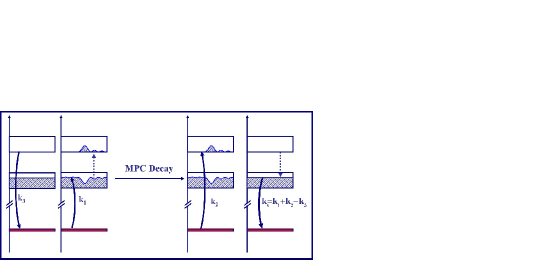
Figure 5: Non-Linear process that gives the MP FWM signal. This corresponds to an inelastic Raman process, assisted by the interactions between the photoexcited Xs and the 2DEG.

The ${\bf k}_{3}$ and ${\bf k}_{1}$ pulses arrive at the same time and photoexcite an inter–LL coherence that subsequently scatters into a MP polarization due to the X–2DEG interactions. The ${\bf k}_{2}$ pulse comes in later and creates an X polarization that scatters off the above decaying MP and gives a signal in the ${\bf k}_{1}+{\bf k}_{2}-{\bf k}_{3}$ direction. In particular, the MP scatters with the photoexcited X into an X state that then recombines to return the system in the ground state. It is interesting to note the similarity of the above process and the familiar one of coherent antiStokes Raman scattering [54] that involves phonons. Note here that, in the case of a spin–polarized 2DEG, the Raman process of excitation and de-excitation of the system with right–circularly polarized light is negligible due the absence of spin–$\downarrow$ electrons in the ground state. A MP excitation can however be excited due to the scattering of the photoexcited spin–$\downarrow$ X with the spin–$\uparrow$ 2DEG. Obviously, if the MP dephases before the ${\bf k}_{2}$ pulse arrives, there will be no FWM signal for this particular sequence of time delays, and therefore the above direction can be used to extract the MP dephasing dynamics from the experimental results. Furthermore, as discussed above, the $\sim\Omega_{M}$ oscillations for $\Delta\tau_{12}=\Delta\tau_{13}>0$ or $\Delta\tau_{12}<0,\Delta\tau_{13}=0$ directions are of quantum kinetic origin and their decay gives important information on the MP coherent dynamics during time scales comparable to the MP period.

Figure 6: TI–FWM signal with PSF + MP contributions when exciting (a) LL0 and LL1 equally (b) mostly LL1 (arbitrary units) The parameters are as in Fig. (1), $W_{M}=W=V_{XX}=3\>meV$, $\gamma_{M}=0.1\>meV$.

Fig. 6 shows the TI signal when both the MP and PSF contributions are included. This figure shows a rich time–dependence, which is dominated by the MP contribution and can be used as a guide to extract from a three–pulse FWM experiment new information about the dephasing dynamics of the $X_{1}$ and $X_{0}$ excitons, as well as the MP dynamics during time scales comparable to the MP period. A comparison between the theory and such an experiment [14] as well as the role of the incoherent effects neglected in the above model will be presented elsewhere.

9 Conclusions

In summary, we discussed a recent theory [7, 9, 10] that provides a unified description of the ultrafast non-linear optical response of magnetoexcitons in both doped and undoped semiconductors, including systems with a strongly correlated many–electron ground state, such as the 2DEG in the QHE regime. We discussed a method for describing the interaction contributions to the density matrix equation of motion, which gives the third–order non-linear polarization measured in transient wave mixing and pump–probe experiments and established the connection with the DCTS treatment of X–phonon and X–X interactions in the undoped system [20, 23, 24]. Using a decomposition of the photoexcited many–body wavefunction into correlated/uncorrelated and excitonic/incoherent contributions, we obtained a factorization scheme for the density matrix that separates out the correlated from the uncorrelated contributions. Importantly, our method applies to systems with a strongly correlated ground state, populated by a 2DEG here, where previous factorization schemes, based on a Hartree–Fock ground state, need to be extended. Our formulation may be used to study the role of exciton–2DEG and exciton–exciton correlations on the ultrafast non-linear optical response and the interplay between coherent and incoherent effects. Our expansion in terms of the optical field is valid for sufficiently short pulses and/or weak excitation conditions, where the correlations are most pronounced. We describe the role of the long–lived collective excitations of a strongly correlated cold electron gas, which is present prior to the optical excitation. We also presented a number of results that describe the Pauli exchange and interaction effects between excitons and magnetoplasmon collective excitations.

We applied our theory to the case of the photoexcitation of the 2DEG with three right–circularly polarized optical pulses. Our numerical solution for the time–integrated three–pulse FWM signal demonstrates a signature of the collective 2DEG excitation dynamics that, for long MP dephasing time, can be distinguished from the Pauli blocking and exciton–exciton interaction contributions. In the case of interest here, the relevant 2DEG collective excitations are the long–lived inter–LL magnetoplasmons, which dress the photoexcited magnetoexcitons and lead to polaronic–like effects and strong non-Markovian dephasing and quantum kinetic effects. We showed that such effects dominate the time delay and frequency dependence of the transient FWM signal in the coherent regime for time scales comparable to the inverse MP frequency. FWM spectroscopy using femtosecond optical pulses provides both the time and the frequency resolution necessary to access a new regime of 2DEG and QHE physics. Our theory allows us to study the experimental signatures of the 2DEG quantum dynamics. We predicted, in particular, strong non-Markovian effects, leading to an asymmetric LL1 exciton lineshape and to strong oscillations as function of time delay of quantum kinetic origin that are governed by the MP dynamics. We also found an optically–induced hybridization of the LL0 and LL1 excitons, with the time–dependent coupling determined by the MP dynamics. A comparison of our results with recent experiments [14] is currently in progress and will be presented elsewhere.

The above correlation–induced non-Markovian dynamics can be controlled by tuning the central frequency of the optical excitation between the two lowest LLs, which changes the coherent admixture of the two MP–dressed magnetoexcitons. FWM experiments using a sequence of optical pulses with different polarizations and central frequencies provide new ways for accessing the very early dynamics of the strongly correlated 2DEG, during time scales shorter than the duration of the interaction processes. This opens up a new window into non-equilibrium Quantum Hall effect physics and collective effects that are just now starting to be explored. In particular, interesting regimes include (1) filling factors away from $\nu=1$, where skyrmions [2] become important in one–sided modulation doped quantum wells and are expected to dominate the magnetoexciton dephasing, and (2) fractional filling factors, where intra–LL collective excitations will dress the magnetoexciton leading to polaronic effects [44].

References

- [1] T. Chakraborty and P. Pietiläinen, The Quantum Hall Effects, Fractional and Integral, second edition (Springer, 1995).
- [2] D. Yoshioka, The Quantum Hall Effect, (Springer-Verlag, 2002).
- [3] See e.g. Perspectives in Quantum Hall Effects, edited by Das Sarma and A. Pinczuk (Wiley, New York, 1997); H. L. Stormer, D. C. Tsui, and A. C. Gossard, Rev. Mod. Phys. 71, S298 (1999).
- [4] See e.g. S. M. Girvin and A. H. MacDonald, in Novel Quantum Liquids in Low Dimensional Semiconductor Structures, edited by S. Das Sarma and A. Pinczuk (Wiley, New York, 1996); N. R. Cooper and D. B. Chklovskii, Phys. Rev. B 55, 2436 (1997); E. H. Aifer, B. B. Goldberg, and D. A. Broido, Phys. Rev. Lett. 76, 680 (1996).
- [5] N. A. Fromer, C. E. Lai, D. S. Chemla, I. E. Perakis, D. Driscoll, and A. C. Gossard, Phys. Rev. Lett. 89, 067401 (2002).
- [6] N. A. Fromer, C. Schüller, D. S. Chemla, T. V. Shahbazyan, I. E. Perakis, K. Maranowski, and A. C. Gossard, Phys Rev. Lett. 83, 4646 (1999).
- [7] A. T. Karathanos, I. E. Perakis, N. A. Fromer, and D. S. Chemla, Phys. Rev B 67, 035316 (2003).
- [8] N. A. Fromer, C. Schüller, C. E. Lai, D. S. Chemla, I. E. Perakis, D. Driscoll, and A. C. Gossard, Phys. Rev. B 66, 205314 (2002).
- [9] I. E. Perakis, Phys. Stat. Sol. B 238, 502 ( 2003).
- [10] I. E. Perakis and D. S. Chemla, Solid State Commun. 127, 147 (2003).
- [11] I. E. Perakis and D. S. Chemla, Phys. Stat. Sol. B 234, 242 ( 2003).
- [12] C. Schueller, I. E. Perakis, N. A. Fromer, and D. S. Chemla, in Nonequilibrium Physics at Short Time Scales: Formation of Correlations, ed. by Klaus Morawetz, 209 (Springer Berlin, Heidelberg, New York, 2004)
- [13] N. A. Fromer, C. Schüller, D. S. Chemla, T. V. Shahbazyan, I. E. Perakis, D. Driscoll, and A. C. Gossard, Physica E 12, 550 (2002).
- [14] K. M. Dani, J. Tignon, M. Breit, D. S. Chemla, E. G. Kavousanaki, A. T. Karathanos, and I. E. Perakis, in Technical Digest, International Quantum Electronics Conference (IQEC), TOPS Vol 97, Optical Society of America (Washington, DC, 2004); and unpublished.
- [15] D. S. Chemla and J. Shah, Nature 411 549 (2001).
- [16] D. S. Chemla, Non-linear Optics in Semiconductors, edited by R. K. Willardson and A. C. Beers (Academic Press, 1999).
- [17] M. Wegener and D. S. Chemla, Chem. Phys. 251, 269 (2000).
- [18] H. Haug and A.–P. Jauho, Quantum Kinetics in Transport and Optics of Semiconductors (Springer, 1996).
- [19] V. M. Axt and T. Kuhn, Rep. Prog. Phys. 67, 433 (2004).
- [20] F. Rossi and T. Kuhn, Rev. Mod. Phys. 74, 895 (2002).
- [21] H. Haug and S. W. Koch, Quantum theory of the optical and electronic properties of semiconductors, 2nd edition (World Scientific, Singapore, 1993).
- [22] J. Shah, Ultrafast Spectroscopy of Semiconductors and Semiconductor Nanostructures (Springer, Heidelberg, 1999).
- [23] V. M. Axt and S. Mukamel, Rev. Mod. Phys. 70, 145 (1998).
- [24] V. M. Axt, K. Victor, and A. Stahl, Phys. Rev. B 53, 7244 (1996).
- [25] J. Schilp, T. Kuhn, and G. Mahler, Phys. Rev. B 50, 5435 (1994).
- [26] N. Donlagic and T. Östreich, Phys. Rev. B 59, 7493 (1999)
- [27] Q. T. Vu, H. Haug, W. A. Hügel, S. Chatterjee, and M. Wegener, Phys. Rev. Lett. 85, 3508 (2000).
- [28] Th. Östreich, K. Schönhammer, and L. J. Sham, Phys. Rev. B 58, 12920 (1998).
- [29] W. Schäfer and M. Wegener, Semiconductor optics and transport phenomena (Springer, Berlin, 2002).
- [30] W. Schäfer, D. S. Kim, J. Shah, T. C. Damen, J. E. Cunningham, K. W. Goossen, L. N. Pfeiffer, and K. Köhler, Phys. Rev. B 53, 16429 (1996).
- [31] R. Lövenich, C. W. Lai, D. Hägele, D. S. Chemla, and W. Scäfer, Phys. Rev. B 66, 045306 (2002)
- [32] R. Binder and S. W. Koch, Prog. Quant. Electron. 19, 307 (1995).
- [33] S. Mukamel, Principles of Non-linear Optical Spectroscopy, (Oxford University Press, 1995).
- [34] I. E. Perakis and T. V. Shahbazyan, Surf. Sci. Reports 40, 1–74 (2000); I. E. Perakis and T. V. Shahbazyan, Int. J. Mod. Phys. B 13, 869–893 (1999); I. E. Perakis, Chem. Phys. 210, 259–277 (1996).
- [35] T. V. Shahbazyan, N. Primozich, and I. E. Perakis, Phys. Rev. B 62, 15925 (2000).
- [36] I. Brener, W. H. Knox, and W. Schaefer, Phys. Rev. B 51, 2005 (1995).
- [37] S. Bar-Ad, I. Bar-Joseph, Y. Levinson, and H. Shtrikman, Phys. Rev. Lett. 72, 776 (1994).
- [38] I. E. Perakis and D. S. Chemla, Phys. Rev. Lett. 72, 3202 (1994).
- [39] I. E. Perakis, I. Brener, W. H. Knox, and D. S. Chemla, J. Opt. Soc. Am. B 13, 1313 (1996).
- [40] N. Primozich, T. V. Shahbazyan, I. E. Perakis, and D. S. Chemla, Phys. Rev. B 61, 2041 (2000).
- [41] T. V. Shahbazyan, N. Primozich, I. E. Perakis, and D. S. Chemla, Phys. Rev. Lett. 84, 2006 (2000).
- [42] R. Haydock, Solid State Phys. 35, 215 (1980); K. Ohno, K. Esfarjani, and Y. Kawazoe, Computational Materials Science (Springer Verlag, Berlin, 1999).
- [43] A. H. MacDonald, J. Phys. C 18, 1003 (1985).
- [44] V. M. Apalkov and E. I. Rashba, Phys. Rev. B 46, 1628 (1992).
- [45] A. Pinczuk in Perspectives in Quantum Hall Effects, edited by Das Sarma and A. Pinczuk (Wiley, New York, 1997).
- [46] A. Pinczuk, B. S. Dennis, D. Heiman, C. Kallin, L. Brey, C. Tejedor S. Schmitt-Rink, L. N. Pfeiffer, and K. W. West, Phys. Rev. Lett. 68, 3623 (1992).
- [47] A. Pinczuk, J. P. Valladares, D. Heiman, A. C. Gossard, J. H. English, C. W. Tu, L. Pfeiffer, and K. West, Phys. Rev. Lett. 61, 2701 (1988).
- [48] I. K. Marmorkos and S. Das Sarma, Phys. Rev. B 45, 13396 (1992).
- [49] S.-R. E. Young, D. A. Broido and L. J. Sham, Phys. Rev. B 32, 6630 (1985); S.-R. E. Young and L. J. Sham, Phys. Rev. Lett. 58, 2598 (1987).
- [50] A. H. MacDonald, H. C. A. Oji and S. M. Girvin, Phys. Rev. Lett. 55, 2208 (1985); H. C. A. Oji and A. H. MacDonald, Phys. Rev. B 33, 3810 (1986).
- [51] C. Kallin and B. I. Halperin, Phys. Rev. B 30, 5655 (1984).
- [52] E. Feenberg, Theory of Quantum Fluids (Academic Press, New York, 1969); R. P. Feynmann, Statistical Mechanics: A Set of Lectures (Benjamin/Cummings, Massachusetts, 1972).
- [53] C. Stafford, S. Schmitt–Rink, and W. Schaefer, Phys. Rev. B 41, 10000 (1990).
- [54] M. Levenson, Introduction to Non-linear Laser Spectroscopy, Acad. Press, New York, (1982).