The directional contact distance of two ellipsoids: Coarse-grained potentials for anisotropic interactions

Abstract

We obtain the distance of closest approach of the surfaces of two arbitrary ellipsoids valid at any orientation and separation, measured along their inter-center vector. This directional distance is derived from the Elliptic Contact Function. The geometric meaning behind this approach is clarified. An elliptic pair potential for modelling arbitrary mixtures of elliptic particles, whether hard or soft, is proposed based on this distance. Comparisons to Gay-Berne potentials are discussed. Analytic expressions for the forces and torques acting on the elliptic particles are given.

I Introduction

Self-assembling systems of current interest in such diverse areas as molecular electronic materials to biological systems often involve molecular units or supra-molecular structures that are highly anisotropic in shapeHartgerink et al. (2001). Typical examples range from lipids in biological membranes Brannigan et al. (2004), to alkanethiols in self-assembled monolayers Love et al. (2005), to carbon nanotubes and inorganic nanorods S.Tsonchev et al. (2003). In the interplay between accuracy, and, simplicity and computational efficiency, such fairly rigid units are often approximated as ellipsoids.

The importance of the geometrical anisotropy in pair-wise interactions has been recognised early on. Berne and Pechukas introduced the Gaussian Overlap Potential (GOP) B.J.Berne and P.Pechukas (1972) whose generalisation led to the widely used Gay-Berne potential (GB) J.G.Gay and B.J.Berne (1981). The main idea behind this approach is the representation of a pair of particles by their joint elliptically stretched Gaussian distribution centered around the molecular centroids. The GB potential has been extensively used for the modelling of the phase behaviour of liquid crystals G.R.Luckhurst and P.S.J.Simmonds (1993). There is renewed interest in the possibility to study dynamical behaviour, as for example in lipids in biological membranes G.Ayton et al. (2001), and in side-chains in coarse-grained protein force-fields A.Liwo et al. (1997). Part of the appeal of the form of the GB potential is that it allows for analytic derivation of forces and torques S.Saraman and D.J.Evans (1993) acting on the particles which simplifies the modelling. The drawbacks are its lack of generality: for example, in its original form, it is only applicable to identical uniaxial elliptic particles, although it has been recently extended for the special case of particles with biaxial symmetry D.J.Cleaver et al. (1996). Another extension of the GB potential was made for an ”ellipsoid in the sea of spheres” scenario S.Ravichandran and B.Bagchi (1999), where the main semi-axis of an elliptic particle is much bigger than the radius of the spherical particles interacting with it. However, as the geometry of the particles vary, so do the number and value of the parameters introduced in the potentials.

A different approach to this problem relies on the Elliptic Contact Function (ECF) introduced by Perram and coworkers J.W.Perram and M.S.Wertheim (1985); J.W.Perram et al. (1996) which emphasises its geometrical aspects. The ECF approach calculates the distance of closest approach of two ellipsoids with given orientations. It gives the correct position of contact when the two ellipsoids are in tangent contact. Therefore it is often referred to as the ”hard ellipsoids” approach. It exploits the algebra behind the representation of ellipsoids as quadratic forms to write the problem as an optimisation task that can be solved efficiently. The GOP potential is known to be closely related to the Elliptic Contact Potential (ECP) derived from the ECF J.W.Perram et al. (1996); D.J.Cleaver et al. (1996); M.P.Allen et al. (1993).

Although applicable to any mixture, the ECF has not yet been widely used in applications. The reasons may be due to the lack of simplicity of the ECF approach and the lack of clarity of its geometric interpretation. Furthermore, the potential derived from this approach has several drawbacks: it does not distinguish in energy between different relative orientations, it does not become isotropic at large separations and it artificially keeps the elliptic shape of the potential along the longer semi-axes of the ellipsoids. In this work, we clarify the geometric meaning of the ECF approach and the parameters associated with it. We show how the true distance of closest approach of the surfaces of two ellipsoids can be approximated well directly from the ECF by the directional distance of closest approach along their inter-center direction $R$. This allows us to develop a new type of elliptic potential applicable for mixtures of ellipsoids and/or spheres. We show that this can be done for any size, any orientation, and ”hard” or ”soft” particles. In all cases, the potential behaves isotropically at infinite separations and addresses the drawbacks discussed above. A comparison with the GB potentials is also presented. Finally, we derive analytical expressions for the appropriate forces and torques that make Molecular Dynamics (MD) simulations possible.

In Section II we give the preliminaries, namely review the main aspects of the ECF from the literature, in Section III we show how to obtain the directional distance of closest approach of two ellipsoids by the value of the ECF and compare it to the GB potentials. In Section IV we show how it leads to a LJ-type of elliptic potential and in Section V we derive analytic expressions for the forces and torques acting on the particles due to the suggested potential. Finally, in Section VI we discuss the implications of this approach and comment on its advantages and drawbacks.

II Preliminaries: the Elliptic Contact Function (ECF)

The shapes of two anisotropic particles ”A” and ”B” centred at points $\bm{r}$ and $\bm{s}$ are represented by the ellipsoids ${\cal A}(\bm{x})=1$ and ${\cal B}(\bm{x})=1$, respectively (Fig. 1). ${\cal A}(\bm{x})$ and ${\cal B}(\bm{x})$ are quadratic forms given by

$${\cal A}(\bm{x})=(\bm{x}-\bm{r})\cdot\bm{A}\cdot(\bm{x}-\bm{r})$$

and

$${\cal B}(\bm{x})=(\bm{x}-\bm{s})\cdot\bm{B}\cdot(\bm{x}-\bm{s}).$$

The matrices $\bm{A}$ and $\bm{B}$ can be expressed as

$$\bm{A}=\sum_{i=1,2,3}a_{i}^{-2}\bm{u}_{i}\otimes\bm{u}_{i},\quad\bm{B}=\sum_{i=1,2,3}b_{i}^{-2}\bm{v}_{i}\otimes\bm{v}_{i}\,,$$ (1)

where $\bm{u}_{i}$ are the unit orthogonal vectors along the three semi-axes of ellipsoid ”A” with lengths $a_{i}$ and, $\bm{v}_{i}$ are the unit orthogonal vectors along the semi-axes of ellipsoid ”B” with lengths $b_{i}$. The symbol ”$\otimes$” in (1) is used to define the matrices $\bm{A}$ and $\bm{B}$ in dyadic form.

The ECF is a measure of proximity of two ellipsoids, originally presented in J.W.Perram et al. (1996) and subsequently reformulated in J.W.Perram (2003). The equivalence of the two definitions is shown in Appendix A. We begin with the latter formulation because it allows us to obtain a clear geometrical interpretation. To this end, we define ${\cal S}(\bm{x},\lambda)$ as an affine combination of quadratic forms ${\cal A}(\bm{x})$ and ${\cal B}(\bm{x})$,

$${\cal S}(\bm{x},\lambda)=\lambda{\cal A}(\bm{x})+(1-\lambda){\cal B}(\bm{x})\,,$$ (2)

where $\lambda$ is a parameter from the interval $[0,1]$. The ECF is defined as a solution to the following optimisation problem:

$$F(\bm{A},\bm{B})=\mathop{\it max}_{\lambda}\mathop{\it min}_{\bm{x}}{\cal S}(\bm{x},\lambda).$$ (3)

The minimum $\bm{x}(\lambda)$ of ${\cal S}(\bm{x},\lambda)$ for each value of the parameter $\lambda$ can be found from

$$\nabla{\cal S}(\bm{x},\lambda)=2\left\{\lambda\bm{A}\cdot(\bm{x}-\bm{r})+(1-\lambda)\bm{B}\cdot(\bm{x}-\bm{s})\right\}=0$$ (4)

as:

$$\bm{x}(\lambda)=\left\{\lambda\bm{A}+(1-\lambda)\bm{B}\right\}^{-1}\cdot\left\{\lambda\bm{A}\cdot\bm{r}+(1-\lambda)\bm{B}\cdot\bm{s}\right\}.$$ (5)

As a result, the optimisation problem given by Eq.3 is simplified to an unconstrained maximisation of the scalar function ${\cal S}(\bm{x}(\lambda),\lambda)$ by the scalar parameter $\lambda$:

$$F(\bm{A},\bm{B})=\mathop{\it max}_{\lambda}{\cal S}(\bm{x}(\lambda),\lambda).$$ (6)

Note that the curve $\bm{x}(\lambda):\lambda\in[0,1]$ with $\bm{x}(0)=\bm{s}$ and $\bm{x}(1)=\bm{r}$ connects the centres $\bm{r}$ and $\bm{s}$ of the two ellipsoids, as can be seen in Fig 1. Along this curve, the gradient vectors $\nabla{\cal A}(\bm{x})$ and $\nabla{\cal B}(\bm{x})$ are parallel. We will find later the following notation useful

$$\lambda\nabla{\cal A}(\bm{x}(\lambda))=2\lambda\bm{A}\cdot(\bm{x}(\lambda)-\bm{r})=\bm{X}(\lambda)\,,$$ (7)

$$(1-\lambda)\nabla{\cal B}(\bm{x}(\lambda))=2(1-\lambda)\bm{B}\cdot(\bm{x}(\lambda)-\bm{s})=-\bm{X}(\lambda).$$

Earlier, it was shown (J.W.Perram and M.S.Wertheim (1985)) that the function ${\cal S}(\bm{x}(\lambda),\lambda)$ has a unique maximum on the interval $\lambda\in(0,1)$. The value $\lambda_{c}$ at which the function reaches its maximum is called the contact parameter and the point $\bm{x}_{c}=\bm{x}(\lambda_{c})$ is called the contact point. The derivative of the function ${\cal S}(\bm{x}(\lambda),\lambda)$ with respect to $\lambda$ is

$${\cal S}^{\prime}(\bm{x}(\lambda),\lambda)=\left\{{\cal A}(\bm{x}(\lambda))-{\cal B}(\bm{x}(\lambda))\right\}+$$

$$2\bm{x}^{\prime}(\lambda)^{T}\cdot\left\{\lambda\bm{A}\cdot(\bm{x}(\lambda)-\bm{r})+(1-\lambda)\bm{B}\cdot(\bm{x}(\lambda)-\bm{s})\right\}.$$ (8)

The term in the second curly braces vanishes along the curve $\bm{x}(\lambda)$ due to Eq. (4). Hence, at the extremum,

$${\cal S}^{\prime}(\bm{x}_{c},\lambda_{c})={\cal A}(\bm{x}_{c})-{\cal B}(\bm{x}_{c})=0\,,$$ (9)

from which we can see that the contact point $\bm{x}_{c}$ is the intersection of the curve $\bm{x}(\lambda)$ with the surface ${\cal A}(\bm{x})={\cal B}(\bm{x})$ (Fig. 1). Eq.9 leads to

$${\cal A}(\bm{x}_{c})={\cal B}(\bm{x}_{c}).$$ (10)

Substitution of the last equation back into Eq. (2) gives the following simple interpretation of the ECF value

$$F(\bm{A},\bm{B})={\cal A}(\bm{x}_{c})={\cal B}(\bm{x}_{c}).$$ (11)

The contact point $\bm{x}_{c}$ lies on the ellipsoid ${\cal A}(\bm{x})=F(\bm{A},\bm{B})$ due to Eq. (11). Similarly for ${\cal B}(\bm{x})$ the contact point $\bm{x}_{c}$ lies on the ellipsoid ${\cal B}(\bm{x})=F(\bm{A},\bm{B})$. The two ellipsoids are in tangent contact (Fig. 1) due to Eq. (4). As a result, the value of the ECF serves as a criterion of approach of any two elliptic particles. If the value $F(\bm{A},\bm{B})$ is below unity, then the original ellipsoids ${\cal A}(\bm{x})=1$ and ${\cal B}(\bm{x})=1$ overlap and vice versa. When $F(\bm{A},\bm{B})$ is equal to one, the original ellipsoids ”A” and ”B” are in tangent contact.

The contact parameter $\lambda_{c}$ can be found numerically as a solution of Eq. (10) by approaching the surface ${\cal A}(\bm{x})={\cal B}(\bm{x})$ along the curve $\bm{x}(\lambda)$:

$$\lambda_{c}:{\cal A}(\bm{x}(\lambda_{c}))-{\cal B}(\bm{x}(\lambda_{c}))=0.$$ (12)

The convergence of this iterative process is usually fast. Numerical aspects of this iterative process as well as ways to speed it up will be discussed elsewhere.

The value of the ECF can be further expressed in the form $F(\bm{A},\bm{B})=R^{2}\,f(\bm{A},\bm{B})$, where $R$ is the inter-center distance between particles ”A” and ”B” (See Appendix A) and $f$ depends only on orientation, which leads to the definition of the Perram-Wertheim (PW) range parameter $\sigma_{PW}(\bm{A},\bm{B})$ (D.J.Cleaver et al. (1996)) as:

$$\sigma_{PW}(\bm{A},\bm{B})=\frac{R}{\sqrt{F(\bm{A},\bm{B})}}=\frac{1}{\sqrt{f(\bm{A},\bm{B})}}.$$ (13)

There is a well-known close relationship J.W.Perram et al. (1996); D.J.Cleaver et al. (1996) between this parameter and the Berne-Pechukas (BP) range parameter, $\sigma_{BP}(\bm{A},\bm{B})$, first introduced in B.J.Berne and P.Pechukas (1972) for the GOP. $\sigma_{BP}(\bm{A},\bm{B})$ can be expressed in terms of ${\cal S}(\bm{x}(\lambda),\lambda)$ (see Appendix B) by substituting $\lambda_{c}=1/2$,

$$\sigma_{BP}(\bm{A},\bm{B})=\frac{R}{\sqrt{{\cal S}(\bm{x}(1/2),1/2)}}.$$ (14)

The BP range parameter is sometimes considered as a mean value approximation of the PW range parameter D.J.Cleaver et al. (1996); R.Berardi et al. (1995), where $\lambda_{c}$ is approximated by $1/2$ (see Eq. 14). Additionally, Eq. 13 is often treated as the distance of closest approach of two ellipsoids, therefore Eq. (14) is believed to be an approximation of the distance of closest approach (Eq. 15). We will return to this point in Sec. III.3.

III Approximations and geometrical interpretations of the distance of closest approach of two ellipsoids

We now show how to obtain the distance of closest approach of the surfaces of two ellipsoids using the ECF value. The true distance of closest approach, $d$, is a solution of the following minimisation problem

$$d(\bm{A},\bm{B})=\mathop{\it min}_{\tilde{\bm{x}}_{a},\tilde{\bm{x}}_{b}}||\tilde{\bm{x}}_{a}-\tilde{\bm{x}}_{b}||,$$ (15)

subject to two constraints

$${\cal A}(\tilde{\bm{x}}_{a})=1,\quad{\cal B}(\tilde{\bm{x}}_{b})=1,$$ (16)

namely, that $\tilde{\bm{x}}_{a}$ and $\tilde{\bm{x}}_{b}$ are points on the surface of ellipsoids “A” and “B”, respectively.

We will now show how to approach this distance using the ECF value, both from above using the geometrical properties of the ECF, and from below, using a mechanical analogy.

III.1 The directional contact distance, $d_{R}$

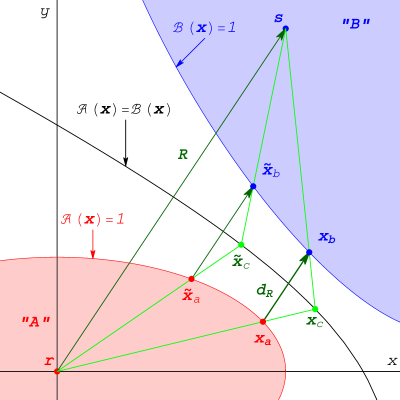
Figure 2: The directional distance of closest approach, $d_{R}(A,B)$, is the minimum distance between the surfaces of two ellipsoids that is parallel to the inter-center vector R. It is given by the sub-contact points $\bm{x}_{a}$ and $\bm{x}_{b}$, which are on the surface of ellipsoids “A” and “B”, respectively. It is a good approximation from above to the true contact distance. The value of the PW approach parameter $\sigma_{PW}(\bm{A},\bm{B})$ can be understood by the geometry of the triangle of points $\bm{r}$, $\bm{s}$ and $\bm{x}_{c}$, as the length of the vector $\bm{R}-(\bm{x}_{a}$- $\bm{x}_{b})$ as soon as $(\bm{x}_{a}$- $\bm{x}_{b})$ becomes parallel to $\bm{R}$

An intersection of the line segment between the contact point $\bm{x}_{c}$ and the center $\bm{r}$ with the surface of the ellipsoid ${\cal A}(\bm{x})=1$ (Fig. 2) can be found using the value $F(\bm{A},\bm{B})$ as:

$$\bm{x}_{a}=\bm{r}+(\bm{x}_{c}-\bm{r})F(\bm{A},\bm{B})^{-1/2}.$$ (17)

The point $\bm{x}_{a}$ will be called a sub-contact point of A. The sub-contact point of B, $x_{b}$ can be found in the same way, namely as the intersection of the line segment between points $\bm{x}_{c}$ and $\bm{s}$ with the surface of the ellipsoid ${\cal B}(\bm{x})=1$

$$\bm{x}_{b}=\bm{s}+(\bm{x}_{c}-\bm{s})F(\bm{A},\bm{B})^{-1/2}.$$ (18)

The vector $(\bm{x}_{b}-\bm{x}_{a})$ between the sub-contact points of A and B is parallel to the inter-center vector $\bm{R}$ and is given by

$$(\bm{x}_{b}-\bm{x}_{a})=(\bm{s}-\bm{r})(1-F(\bm{A},\bm{B})^{-1/2})=\hat{\bm{R}}\,d_{R}(\bm{A},\bm{B})\,,$$ (19)

where

$$d_{R}(\bm{A},\bm{B})=R(1-F(\bm{A},\bm{B})^{-1/2})=R-\sigma_{PW}(\bm{A},\bm{B}).$$ (20)

The geometrical meaning of the PW range parameter becomes now clear from Eq. (20): it is the sum of projections of vectors $(\bm{x}_{a}-\bm{r})$ and $(\bm{s}-\bm{x}_{b})$ on the inter-particle vector $\bm{R}$ or simply the length of the vector $\bm{R}-(\bm{x}_{b}-\bm{x}_{a})$ as soon as $(\bm{x}_{b}-\bm{x}_{a})$ is parallel to $\bm{R}$ (Fig. (2)). The distance $d_{R}$ (Eq. 20) has a meaning of the shortest directional distance between two ellipsoids measured along the direction of their inter-particle vector $\bm{R}$.

To see this note that on the surface ${\cal A}(\bm{x})={\cal B}(\bm{x})$ any affine combination ${\cal S}(\bm{x},\lambda)$ with any value of the parameter $\lambda$ is equal to both ${\cal A}(\bm{x})$ and ${\cal B}(\bm{x})$. At the same time for $\lambda=\lambda_{c}$ we have shown, that ${\cal S}(\bm{x},\lambda_{c})$ reaches it’s minimum at the contact point $\bm{x}_{c}$. As a result, the optimisation problem (3)-(2) can be reformulated as a problem of finding the minimum of ${\cal A}(\bm{x})$ or ${\cal B}(\bm{x})$ on the surface ${\cal A}(\bm{x})={\cal B}(\bm{x})$.

Note that Eqs. (17) and (18) hold not only for the contact point $\bm{x}_{c}$ but for any point $\tilde{\bm{x}}_{c}$ (see Fig. 2) on the surface ${\cal A}(\bm{x})-{\cal B}(\bm{x})=0$ in the following way:

$$\tilde{\bm{x}}_{a}=\bm{r}+(\tilde{\bm{x}}_{c}-\bm{r}){\cal S}(\tilde{\bm{x}}_{c})^{-1/2}\,,$$ (21)

$$\tilde{\bm{x}}_{b}=\bm{s}+(\tilde{\bm{x}}_{c}-\bm{s}){\cal S}(\tilde{\bm{x}}_{c})^{-1/2}\,,$$ (22)

where ${\cal S}(\bm{x})$ means here any affine combination of ${\cal A}(\bm{x})$ and ${\cal B}(\bm{x})$. The resulting vector $(\tilde{\bm{x}}_{b}-\tilde{\bm{x}}_{a})$ is also parallel to the inter-particle vector $\bm{R}$ (Fig. 2).

$$(\tilde{\bm{x}}_{b}-\tilde{\bm{x}}_{b})=\bm{R}(1-{\cal S}(\tilde{\bm{x}}_{c})^{-1/2}).$$ (23)

The minimum of the value ${\cal S}(\tilde{\bm{x}}_{c})$ is $F(\bm{A},\bm{B})$. It is easy to show, that the value $(1-{\cal S}(\tilde{\bm{x}}_{c})^{-1/2})$ reaches its minimum together with ${\cal S}(\tilde{\bm{x}}_{c})$. As a result, the distance $d_{R}(\bm{A},\bm{B})$ has a meaning of minimum length of the vector $(\tilde{\bm{x}}_{b}-\tilde{\bm{x}}_{a})$ parallel to $\bm{R}$.

If we consider the value $d_{R}(\bm{A},\bm{B})$ as a minimum distance along any arbitrary direction independently from the inter-particle vector, then its minimum among all possible directions naturally is the distance of closest approach of two ellipsoids $d(\bm{A},\bm{B})$. As a result the following inequality holds while $d(\bm{A},\bm{B})$ is greater than zero:

$$d(\bm{A},\bm{B})\leq d_{R}(\bm{A},\bm{B})\,.$$ (24)

III.2 The distance from below, $d_{n}$

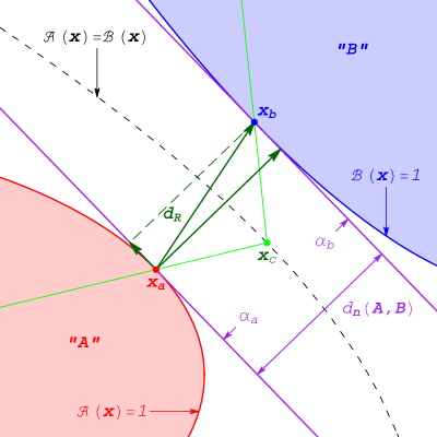
Figure 4: A closer look at the sub-contact points $\bm{x}_{a}$ and $\bm{x}_{b}$, which define the directional distance of closest approach $d_{R}$. The planes $\alpha_{a}$ and $\alpha_{b}$ are tangent to the ellipsoids ${\cal A}(\bm{x})=1$ and ${\cal B}(\bm{x})=1$ respectively at these points (shown with purple lines). The distance $d_{n}$ approaches the true distance of closest approach from below, while $d_{R}$ approaches it from above.

An estimation of the distance of Eq. (15) from below is given by the distance between two parallel planes $\alpha_{a}$ and $\alpha_{b}$, which are tangent to ellipsoids ”A” and ”B” at the sub-contact points $\bm{x}_{a}$ and $\bm{x}_{b}$ (Fig. 4):

$$d_{\bm{n}}(\bm{A},\bm{B})=\hat{\bm{X}}_{c}\cdot(\bm{x}_{b}-\bm{x}_{a})=\hat{\bm{X}}_{c}\cdot\bm{R}\,(1-F(\bm{A},\bm{B})^{-1/2})\,,$$ (25)

where $\hat{\bm{X}}_{c}$ is the unit vector in the direction of the gradient vector (Eq. 7)

$$\hat{\bm{X}}_{c}=\frac{\bm{X}_{c}}{||\bm{X}_{c}||}=\frac{\nabla{\cal A}(\bm{x}_{a})}{||\nabla{\cal A}(\bm{x}_{a})||}=-\frac{\nabla{\cal B}(\bm{x}_{b})}{||\nabla{\cal B}(\bm{x}_{b})||}.$$

In fact, the maximum of the distance (25) among all possible positions of points $\tilde{\bm{x}}_{A}$ and $\tilde{\bm{x}}_{B}$ on the surfaces of ellipsoids ”A” and ”B”, such that the tangent planes $\alpha_{a}$ and $\alpha_{b}$ are parallel, is equal to the true contact distance $d(\bm{A},\bm{B})$ as long as the ellipsoids ”A” and ”B” are not overlapping.

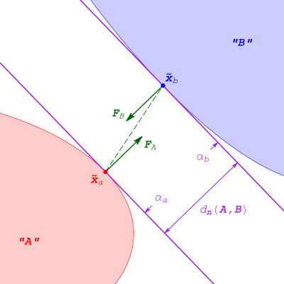
Figure 3: The distance $d_{n}(A,B)$ is defined as the distance between two parallel planes $\alpha_{a}$ and $\alpha_{b}$ which are tangent at any point $\tilde{\bm{x}_{a}}$ and $\tilde{\bm{x}_{b}}$ on the surface of ellipsoids “A” and “B”, respectively. It approaches the true distance of closest approach from below. The maximum distance $d_{n}(A,B)\textsterling$ coincides with the true distance of closest approach. This can be understood from a mechanical point of view: if the planes are kept apart by a constant force ${\bf F}$, then the equilibrium point reached corresponds to the maximum distance between planes, which is also the distance of closest approach.

To show this, we consider a mechanical analogy. We consider the parallel planes $\alpha_{a}$ and $\alpha_{b}$ between two fixed rigid convex bodies ”A” and ”B” which are separated by some distance and kept apart by a constant force $\bm{F}$. The two planes will move away from each other until they touch the bodies ”A” and ”B” at points $\tilde{\bm{x}}_{a}$ and $\tilde{\bm{x}}_{b}$ respectively (see Fig. 3). The reaction forces $\bm{F}_{A}$ and $\bm{F}_{B}$ from the bodies ”A” and ”B” will act on the planes $\alpha_{a}$ and $\alpha_{b}$ along normal vectors of the surfaces of ”A” and ”B” at the points $\tilde{\bm{x}}_{a}$ and $\tilde{\bm{x}}_{b}$. The normal vectors at the surfaces of ”A” and ”B” at $\tilde{\bm{x}}_{a}$ and $\tilde{\bm{x}}_{b}$ are parallel due to the fact that $\alpha_{a}$ and $\alpha_{b}$ are parallel themselves.

The stationary/equilibrium point will be reached when the total force $\bm{F}_{A}+\bm{F}_{B}$ and the total torque $(\bm{x}_{B}-\bm{x}_{A})\times\bm{F}_{B}$ acting on the system of the planes are both equal to zero. The stationary point will correspond to the maximum possible distance between the planes because of the force $\bm{F}$ that is acting to separate them. The total force is always equal to zero $\bm{F}_{A}+\bm{F}_{B}=0$ because $\bm{F}_{A}=\bm{F}$ and $\bm{F}_{B}=-\bm{F}$. The total torque can be equal to zero only if $(\tilde{\bm{x}}_{a}-\tilde{\bm{x}}_{b})$ is parallel to the normal vectors of the surfaces of ”A” and ”B” at $\tilde{\bm{x}}_{a}$ and $\tilde{\bm{x}}_{b}$, which is a solution of the optimisation problem for the distance of closest approach $d(\bm{A},\bm{B})$ (Eq. (15)) as well. As a result the maximum distance between planes $\alpha_{a}$ and $\alpha_{b}$ trapped between two convex bodies is equal to the distance of closest approach of the surfaces of these two bodies.

This leads to

$$0<d_{\bm{n}}(\bm{A},\bm{B})\leq d(\bm{A},\bm{B})\leq d_{R}(\bm{A},\bm{B})\,,$$ (26)

while $d(\bm{A},\bm{B})>0$. All three values $d_{\bm{n}}(\bm{A},\bm{B})$, $d(\bm{A},\bm{B})$ and $d_{R}(\bm{A},\bm{B})$ are equal to zero, when the ellipsoids are in tangent contact

$$0=d_{\bm{n}}(\bm{A},\bm{B})=d(\bm{A},\bm{B})=d_{R}(\bm{A},\bm{B}).$$ (27)

The inequality (26) does not hold when the two ellipsoids overlap. The distance $d(\bm{A},\bm{B})$, the solution of the optimisation task (15)-(16), remains zero whenever ”A” and ”B” overlap. However, the values $d_{R}(\bm{A},\bm{B})$ and $d_{\bm{n}}(\bm{A},\bm{B})$ are below zero and characterise the overlap of the ellipsoids. As a result, the distance $d_{R}(\bm{A},\bm{B})$ can be used in both ”soft” and ”hard” potentials.

In practise, $d_{\bm{n}}(\bm{A},\bm{B})$ is closer to the true distance $d(\bm{A},\bm{B})$ for small separations while $d_{R}(\bm{A},\bm{B})$ is a very good approximation at larger separations and behaves isotropically for infinite separations. Even though the distance $d(\bm{A},\bm{B})$ (15) can be used to build a pair potential between two elliptic particles R.Everaers and M.R.Ejtehadi (2003), the usage of a pair potential based on this distance in molecular simulations is computationally expensive because it requires a solution of the problem (15)-(16) at least once at each integration step for each pair of particles. Although the calculation of the ECF as a proximity measure still involves the solution of the optimisation task (5)-(6) for each pair of particles on each simulation step, the resulting optimisation problem is simpler and computationally more efficient than the problem (15)-(16). Additionally, we will show that the usage of the range parameter of Eq. (13) leads to simple and compact expressions for forces and torques acting on the particles.

III.3 On the relation between the BP and PW range parameters

We can now return to the relation of the BP range parameter as a mean value approximation to the PW range parameter (R.Everaers and M.R.Ejtehadi (2003); D.J.Cleaver et al. (1996)). To examine this further, let’s consider the value of ${\cal S}(\bm{x},\lambda)$ on the curve $\bm{x}(\lambda)$ for different relative orientations. We first consider two identical uniaxial elliptic particles. The GOP and GB potentials were originally introduced for this kind of particles B.J.Berne and P.Pechukas (1972); J.G.Gay and B.J.Berne (1981). We will show that the function ${\cal S}(\bm{x}(\lambda),\lambda)$ becomes symmetric on the interval $\lambda\in\left[0,1\right]$ whenever there is a point or a line or a plane of symmetry between the two ellipsoids. As a result the maximum $F(\bm{A},\bm{B})$ of the function ${\cal S}(\bm{x}(\lambda),\lambda)$ can only occur at $\lambda_{c}=1/2$. Hence, when the quadratic forms ${\cal A}(\bm{x})$ and ${\cal B}(\bm{x})$ are symmetric, the BP range parameter $\sigma_{BP}(\bm{A},\bm{B})$ agrees with the value of the PW range parameter $\sigma_{PW}(\bm{A},\bm{B})$. However, for asymmetric configurations, this is generally not true.

To proceed we express the shape matrix of a spheroid as

$$\bm{A}=l^{-2}\,\bm{u}\otimes\bm{u}+d^{-2}\,(\bm{E}-\bm{u}\otimes\bm{u})\,,$$ (28)

where $2l$ is the length of the ellipsoid, $2d$ its breadth, $\bm{u}$ a unit vector of the the main axis and $\bm{E}$ a unit tensor given by $\bm{E}=\sum\limits_{j=1}^{3}\bm{e}_{j}\otimes\bm{e}_{j}.$ Let’s for simplicity move the origin of the reference frame into a centre of symmetry $\bm{c}$ (this point is not necessarily unique for different types of symmetry). Vectors designating directions and positions in this reference frame are denoted by Greek letters. A vector $\bm{\xi}$ is transformed into its symmetric image $\tilde{\bm{\xi}}$ by a matrix $\bm{\Omega}$ which does not change its length but changes its directions:

$$\tilde{\bm{\xi}}=\bm{\Omega}\cdot\bm{\xi}\,.$$ (29)

For the matrix $\bm{\Omega}$ to be a symmetric transformation, we require the following property:

$$\bm{\Omega}\cdot\bm{\Omega}=\bm{E}\,,$$ (30)

which implies that the determinant of $\bm{\Omega}$ can be $1$ or $-1$.

The quadratic forms ${\cal A}(\bm{x})$ and ${\cal B}(\bm{x})$ are symmetric with respect to the centre of symmetry $\bm{c}$ if the centre $\bm{s}$ of ${\cal B}(\bm{x})$ is a symmetric image of the centre $\bm{r}$ of ${\cal A}(\bm{x})$, so that

$$\bm{r}=\bm{c}+\bm{\eta}\,,\quad\bm{s}=\bm{c}+\tilde{\bm{\eta}}\,,\quad\tilde{\bm{\eta}}=\bm{\Omega}\cdot\bm{\eta}$$ (31)

,and, the matrix $\bm{B}$ is a symmetric image of the matrix $\bm{A}$, satisfying

$$\bm{B}=\bm{\Omega}\cdot\bm{A}\cdot\bm{\Omega}.$$ (32)

Eq. (32) includes in addition the symmetries of particle ”A”.

The possible cases of symmetry of quadratic forms ${\cal A}(\bm{x})$ and ${\cal B}(\bm{x})$ are the point symmetry $\bm{\Omega}=-\bm{E}$, the line symmetry, $\bm{\Omega}=2\,\bm{l}\otimes\bm{l}-\bm{E}$, and the plane symmetry $\bm{\Omega}=\bm{E}-2\,\bm{n}\otimes\bm{n}$, where $\bm{l}$ is a unit vector along the axis of symmetry and $\bm{n}$ is a unit vector normal to the plane of symmetry. In the case of line symmetry, any point of the actual axis of symmetry can serve as a centre of symmetry $\bm{c}$, while in the case of plane symmetry, any point of the plane of symmetry can be considered as a centre of symmetry $\bm{c}$.

Using Eqs. (29)-(32), it can be shown that for any point $\bm{\xi}$ and its image $\tilde{\bm{\xi}}$, the values of the symmetric quadratic forms satisfy the following equations:

$${\cal A}(\bm{\xi})={\cal B}(\tilde{\bm{\xi}}),\quad{\cal A}(\tilde{\bm{\xi}})={\cal B}(\bm{\xi})\,.$$ (33)

The function $S$ of Eq 2 now becomes

$${\cal S}(\bm{\xi},\lambda)=\lambda{\cal A}(\bm{\xi})+(1-\lambda){\cal B}(\bm{\xi})=$$ (34)

$$\lambda{\cal B}(\tilde{\bm{\xi}})+(1-\lambda){\cal A}(\tilde{\bm{\xi}})={\cal S}(\tilde{\bm{\xi}},(1-\lambda))$$

and its gradient is given by

$$\nabla{\cal S}(\tilde{\bm{\xi}},(1-\lambda))=\bm{\Omega}\cdot\nabla{\cal S}(\bm{\xi},\lambda)\,.$$ (35)

From Eq. (35) it follows that, if a point $\bm{\xi}$ belongs to the curve $\bm{x}(\lambda)$ (Eq. (5)), its symmetric image belongs to the curve $\bm{x}(\lambda)$ as well. Further from Eq. (34) it follows that whenever a symmetry described by Eqs. (29)-(32) is present, the function ${\cal S}(\bm{x}(\lambda),\lambda)$ becomes symmetric on the interval $\lambda\in[0,1]$. As a result, the maximum $F(\bm{A},\bm{B})$ of the function ${\cal S}(\bm{x}(\lambda),\lambda)$ can only occur at $\lambda_{c}=1/2$. This shows that the BP and PW parameters are equivalent for symmetric quadratic forms, namely for symmetric configurations of equivalent particles.

If we now inspect the zero level of the GB pair potential depending on the relative orientation of two particles

$$U_{GB}(\bm{A},\bm{B})=0\,,$$ (36)

we can see that the level (36) does not depend on the GB strength parameters (see Appendix B) and it is equivalent to

$$\sigma_{BP}(\bm{A},\bm{B})=1\,,$$ (37)

which is in turn equivalent to

$${\cal S}(\bm{x}(1/2),1/2)=1\,.$$ (38)

In the case of point symmetry the matrix $\bm{B}$ is equal to the matrix $\bm{A}$.

$$\bm{B}=\bm{\Omega}\cdot\bm{A}\cdot\bm{\Omega}=(-\bm{E})\cdot\bm{A}\cdot(-\bm{E})=\bm{A}\,,$$ (39)

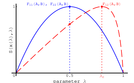
Figure 5: ${\cal S}(\bm{x}(\lambda),\lambda)$ is shown as a function of the parameter $\lambda$ for the “2-to-2” (”side-to-side”), “1-to-1” (”end-to-end”) and “1-to-2” (”side-to-end”) relative orientations of two identical ellipsoids. The ECF value, ${F_{ij}(A,B)}$, is the maximum of the function $S$ and gives the contact parameter $\lambda_{c}$ for each orientation. The approximation of $\lambda_{c}$ by $1/2$ holds for symmetric configurations of identical ellipsoids such as “2-to-2” and “1-to-1”, but fails in the asymmetric “1-to-2” configuration. This is expected to hold for asymmetric configurations in general, which includes any configuration of non-identical particles.

which corresponds to ”perfectly aligned” configurations including ”side-to-side” and ”end-to-end” configurations, which are often used for the adjustment of GOP and GB potentials. (In this work, we use the “i-to-j”notation to refer to the different configurations. For example, “end-to-end” is denoted by “1-to-1”, “side-to-side” by “2-to-2”, “side-to-end” by “1-to-2”.) As a result, the BP range parameter predicts the value of the PW range parameter correctly. However, the “1-to-2” orientation of the molecules is not symmetric and here the approximation $\lambda_{c}=1/2$ fails (Fig. 5). In fact, Eq. (37) will be satisfied when the actual ellipsoids are already separated by some distance above zero due to the fact that in asymmetric configurations the value ${\cal S}(\bm{x}(1/2),1/2)$ is always an underestimation of the ECF value $F(\bm{A},\bm{B})$ (Fig. 5). This means that the size of the molecule given by (36) for the ”side-to-end” configuration (and any other configuration such that $\lambda_{c}\neq 1/2$) will be increased compared to a symmetric configuration (such as ”side-to-side” and ”end-to-end”) of the same molecule and the same potential. Such an increase of the volume of the particles might act as an artificial ”ordering force”, which will force elliptic particles into symmetric (ordered) configurations.

This analysis is of course far from complete. The total pair potential also depends on the GOP strength parameter, so that the resulting deviations of the final shape of the particles are rather complex. In general, we expect the described deviation to grow with the ellipticity of the interacting spheroids. Note, that for unequal elliptic particles, the approximation $\lambda_{c}=1/2$ fails everywhere except for some rare cases.

IV An elliptic potential based on the directional distance, $d_{R}$

We now use the directional distance $d_{R}(\bm{A},\bm{B})$ obtained in Sec.III.1 to construct a new elliptic potential. Here, we concentrate on the LJ 12-6 form as an example of a radial potential.

The LJ potential for two different spherical particles ”A” and ”B” has the following form Allen and Tildesley (1987):

$$U_{LJ}(A,B)=4\epsilon_{AB}\left[\left(\frac{\sigma_{AB}}{\rho_{AB}}\right)^{12}-\left(\frac{\sigma_{AB}}{\rho_{AB}}\right)^{6}\right]\,,$$ (40)

where

$$\sigma_{AB}=(\sigma_{A}+\sigma_{B})/2,\quad\epsilon_{AB}=\sqrt{\epsilon_{AA}\epsilon_{BB}}\,,$$ (41)

and $\rho_{AB}$ is the inter-center distance. Eq. (41) represents the well known Lorentz-Berelot mixing rules for Van-der-Waals radii $\sigma_{A}$ and $\sigma_{B}$ of interacting particles and their depths parameters $\epsilon_{AA}$ and $\epsilon_{BB}$ commonly used in the LJ potential. The parameter $\epsilon_{\alpha\alpha}$ has the meaning of the depth of the potential well for the interaction of two identical particles of type ”$\alpha$”.

The distance $d_{R}(\bm{A},\bm{B})$ can be consistently compared with the inter-center distance $R$. Using Eq. (20), the PW range parameter $\sigma_{PW}(\bm{A},\bm{B})$ can be treated as the sum of radii of two elliptic particles at a given relative orientation. From this point of view, $\sigma_{PW}(\bm{A},\bm{B})$ can be considered as an orientation-dependent ”mixing rule” for two elliptic particles similar to $\sigma_{AB}$ in Eq.41. Using this analogy, the following elliptic potential can be built in Lennard-Jones form:

$$U=4\epsilon_{0}\left[\left(\frac{R\,F(\bm{A},\bm{B})^{-1/2}}{R}\right)^{12}-\left(\frac{R\,F(\bm{A},\bm{B})^{-1/2}}{R}\right)^{6}\right]=$$

$$4\epsilon_{0}\left[F(\bm{A},\bm{B})^{-6}-F(\bm{A},\bm{B})^{-3}\right]\,,$$ (42)

which is the Elliptic Contact Potential (ECP) developed by Perram and co-workers J.W.Perram and M.S.Wertheim (1985); J.W.Perram et al. (1996). We can now see that this potential is a consistent generalisation of the Lennard-Jones potential in the case of elliptic particles when one considers the inter-particle distance $R$ together with the ”mixing rule” $\sigma_{PW}(\bm{A},\bm{B})$. The value $\epsilon_{0}$ has the meaning of the potential minimum.

However, the potential (42) in this form has several disadvantages. First of all, it does not become isotropic at large separations of the particles. Secondly, the depth of the potential minimum remains the same for all relative orientations of the particles ”A” and ”B”. And lastly, the shape of the potential well is not realistic because it is wider along the longer semi-axes of the ellipsoids than the original potential. These disadvantages prevent the potential of Eq. (42) from being extensively used in applications. Here, we would like to build an extension to the ECP, which preserves the good features of the ECF approach but frees it from the disadvantages mentioned above.

These problems come from the ”Lennard-Jones like” reduced distance $(R/\sigma_{PW}(\bm{A},\bm{B}))$ used in the ECP (Eq. 42). This distance becomes one when the ellipsoids are in contact and the potential goes to zero and keeps an ”elliptic shape” at large separations that causes both the unrealistic anisotropy of the ECP at long distances and the unrealistic shape of the potential well. However, the directional distance $d_{R}(\bm{A},\bm{B})$ along the inter-particle vector itself becomes isotropic at large separations. Using this distance instead, a ”shifted form” of the potential (42) can be built as:

$$U(\bm{A},\bm{B})=4\epsilon_{0}\left[\left(\frac{\sigma_{0}}{d_{R}(\bm{A},\bm{B})+\sigma_{0}}\right)^{12}-\left(\frac{\sigma_{0}}{d_{R}(\bm{A},\bm{B})+\sigma_{0}}\right)^{6}\right]=$$

$$4\epsilon_{0}\left[\left(\frac{\sigma_{0}}{R-R\,F(\bm{A},\bm{B})^{-1/2}+\sigma_{0}}\right)^{12}-\left(\frac{\sigma_{0}}{R-R\,F(\bm{A},\bm{B})^{-1/2}+\sigma_{0}}\right)^{6}\right],$$ (43)

where $\sigma_{0}$ has the meaning of characteristic length and is responsible for the width of the potential well. The shape of the potential well is now more realistic because the distance $d_{R}(\bm{A},\bm{B})$ is a good approximation to the distance $d(\bm{A},\bm{B})$. The potential (43) has the form of the GB potential without a strength parameter and the PW range parameter instead of the GOP one J.G.Gay and B.J.Berne (1981).

The depth of the wells of the potential (43) however still equals one in any direction. One way to allow for variable depth of the potential minima is to use different shape matrices for the attractive and the repulsive part of the potential of Eq.(43)

$$U(\bm{A}_{1},\bm{A}_{2},\bm{B}_{1},\bm{B}_{2})=$$

$$4\epsilon_{0}\left[\left(\frac{\sigma_{0}}{R-R\,F_{1}(\bm{A}_{1},\bm{B}_{1})^{-1/2}+\sigma_{0}}\right)^{12}-\left(\frac{\sigma_{0}}{R-R\,F_{2}(\bm{A}_{2},\bm{B}_{2})^{-1/2}+\sigma_{0}}\right)^{6}\right],$$ (44)

where the ”repulsive ECF” $F_{1}(\bm{A}_{1},\bm{B}_{1})$ and the ”attractive ECF” $F_{2}(\bm{A}_{2},\bm{B}_{2})$ are calculated using different shape matrices

$$\bm{A}_{1}=\sum_{i=1,2,3}a_{1i}^{-2}\bm{u}_{i}\otimes\bm{u}_{i},\quad\bm{B}_{1}=\sum_{i=1,2,3}b_{1i}^{-2}\bm{v}_{i}\otimes\bm{v}_{i},$$ (45)

and

$$\bm{A}_{2}=\sum_{i=1,2,3}a_{2i}^{-2}\bm{u}_{i}\otimes\bm{u}_{i}\quad\bm{B}_{2}=\sum_{i=1,2,3}b_{2i}^{-2}\bm{v}_{i}\otimes\bm{v}_{i}\,.$$ (46)

A justification for this approach can be given by inspecting the constant levels of the attractive and repulsive parts of a pair potential of two complex molecules, calculated as the sum of attractive and repulsive parts of the LJ potentials of spherical particles. It is easy to see that the constant levels $LJ_{12}$ and $LJ_{6}$ do have close but different shapes.

Although this introduces more parameters to the problem, the total number of fitting parameters is still reduced compared to the GB potential. For example, the empirical exponents $\nu$ and $\mu$ present in the GB potential (see Appendix B) are excluded. Additionally, the small deviation of the attractive shape matrices $\bm{A}_{2}$ and $\bm{B}_{2}$ with respect to the repulsive ones $\bm{A}_{1}$ and $\bm{B}_{1}$ allows us in practise to use the solution of the ”attractive” ECF problem- $\lambda_{c2}$ and $\bm{x}_{c2}$- as the initial conditions for the ”repulsive” ECF problem, which reduces the number of iterations required for the calculation of the latter. Besides, when calculated separately, the repulsive ECF problem requires a much smaller cut-off value. As a result both ECF problems are solved only when molecules are very close.

To illustrate the form of the potential we consider two examples.

IV.1 Example 1

As a simple test case, we consider the pair potential of two identical spheroids consisting of 6 LJ spherical particles in a linear array J.G.Gay and B.J.Berne (1981). The resulting fitted potential and the target LJ potential are shown in Fig. 6. Although only the values of ”side-to-side” and ”end-to-end” potential minima are fitted, the ”side-to-end” configuration is also close to the target potential. The “2-2” or “side-to-side” potential minimum of such potential is $min_{R}U_{22}=14.883$ when the LJ parameters are $\sigma=1$, $\epsilon=1$, and the spheres are separated by a distance of $2/3.$ and has been set to unity. Therefore a strength parameter $\epsilon=14.883$ should be used in simulations.

For identical uniaxial particles there is the possibility for further reduction of the number of the fitting parameters. The choice of ”i-th” ”attractive semi-axes” equal to ”i-th” ”repulsive semi-axes”

$$a_{1i}=b_{1i}=a_{2i}=b_{2i}$$ (47)

leaves the corresponding ”i-to-i” potential minimum equal to one as expected. Then the parameter $\epsilon_{0}$ in Eq. (43) has the meaning of the ”i-to-i” potential minimum. As a result, the adjustment of the pair potential (43) for identical spheroids requires in total 5 fitting parameters, while in the GB potential 8 parameters are used.

The same reduction can be used for unequal and biaxial particles as well, but then the fitting of the potential to a target potential become less flexible in the representation of ratios of different potential minima.

IV.2 Example 2

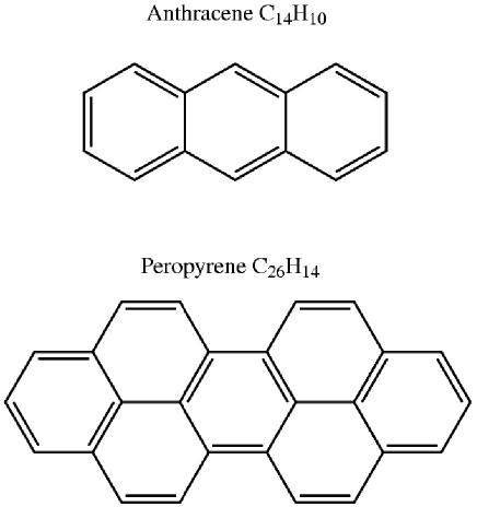
Figure 7: The test molecules of the unequal biaxial case: peropyrene, $C_{26}H_{14}$, and anthracene, $C_{14}H_{10}$.

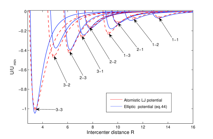
Figure 8: ”i-to-j” potential minima of the peropyrene-anthracene LJ atomic pair potential (red dashed lines - - -) fitted with the suggested potential of Eq. IV (blue solid curves-). The fit was done with a weighted sum of squares difference which in this case gave more weight to the accuracy of the “aligned” configurations “1-to-1”,”2-to-2” and “3-to-3”. This choice would depend on the particular application. The following LJ parameters were used for hydrogen, H, and carbon, C,: $\sigma_{HH}=2.4\AA,\epsilon_{HH}=0.02$ kcal/mol, $\sigma_{CC}=3.4\AA,\epsilon_{CC}=0.15$ kcal/mol. The resulting repulsive shape matrix elements for $\bm{A}_{1}$ and $\bm{B}_{1}$ are $a_{11}=7.024,a_{12}=4.006,a_{13}=1.582$ and $b_{11}=4.846,b_{12}=2.841,b_{13}=1.511$, while the attractive shape matrix elements for $\bm{A}_{2}$ and $\bm{B}_{2}$ are given by $a_{21}=6.528,a_{22}=3.829,a_{23}=1.702,b_{21}=4.267,b_{22}=2.405,b_{23}=1.394$, with width parameter $\sigma_{0}=2.921$ and depth parameter $\epsilon=25.543$.

We consider a more complicated example, namely the pair interaction of two non-identical biaxial molecules, peropyrene $C_{26}H_{14}$ and anthracene $C_{14}H_{10}$ (Fig. 7). The peropyrene-to-anthracene pair potential is calculated as a sum of LJ interactions between all atoms of the molecules after a geometry optimisation of the isolated molecules Frisch et al. (2003). Considering only cases where the ”i-th” semi-axis of the particle ”A” is aligned with the ”j-th” semi-axis of the particle ”B”, there are in total 9 ”i-to-j” configurations which need to be represented. The objective function for the least-squares fitting was built as a weighted sum of square differences of the potential minimum value, the position of the root $U(\bm{A},\bm{B})=0$ and the width of the potential well at half-depth for each of the ”i-to-j” relative orientations of the molecules. In this example, the relative weights were chosen to represent ”aligned” configurations ”1-to-1”, ”2-to-2” and ”3-to-3” more accurately then other ”misaligned” configurations. However, the particular choice of the weights can be made to suite an application in mind. The target potential was averaged over rotations of the molecules about their inter-center vector $\bm{R}$ for each ”i-to-j” configuration. Fig. (8) shows that the potential (IV) is able to reproduce, at least qualitatively, the complex interaction profile of the peropyrene-anthracene pair potential. This is encouraging since $d_{R}$ is more accurate at longer separations rather than at short but the wells around the minima are still reasonably well represented.

V Derivation of forces and torques

The dynamical evolution of the system via Molecular Dynamics (MD) simulations requires the calculation of forces and torques acting on the particles due to their interactions with all other particles. The suitability of a reduced representation potential for MD simulations is mainly defined by the computing time spent on the calculation of forces and torques due to that potential. A numerical estimation of the derivatives of the potential is computationally expensive. Additionally, approximate values of the derivatives is an extra source for numerical errors. The possibility of expressing those derivatives analytically is a big advantage for a reduced representation potential.

In this Section we derive analytic expressions for the forces and torques acting on the elliptic particles due to the suggested potential (IV) that allow for efficient MD simulations to be performed. The resulting formulae are simple due to the simple structure of the potential (IV) and the extremum properties of the ECF value (6).

The following notation will be used:

$$U_{AB}=U(\bm{A}_{1},\bm{A}_{2},\bm{B}_{1},\bm{B}_{2}),$$ (48)

$$F_{i}=F_{i}(\bm{A}_{i},\bm{B}_{i}),$$

$$\bm{X}_{c}=\bm{X}(\lambda_{c}).$$

Given

$$U_{AB}=4\epsilon_{0}\left[G_{1}^{-12}-G_{2}^{-6}\right]\,,$$ (49)

where

$$G_{i}=(R-RF_{i}^{-1/2}+\sigma_{0})/\sigma_{0},$$ (50)

the force acting on particle ”A” is

$$\bm{F}_{A}=-\frac{d\,U_{AB}}{d\,\bm{r}}=24\epsilon_{0}\left[2\,G_{1}^{-13}\,\frac{d\,G_{1}}{d\,\bm{r}}-G_{2}^{-7}\,\frac{d\,G_{2}}{d\,\bm{r}}\right]\,,$$ (51)

where

$$\frac{d\,G_{i}}{d\,\bm{r}}=\frac{1}{\sigma_{0}}\left[\hat{\bm{R}}(F_{i}^{-1/2}-1)+\frac{R}{2}\,F_{i}^{-3/2}\frac{d\,F_{i}}{d\,\bm{r}}\,\right]\,,$$ (52)

and

$$\frac{d\,F_{i}}{d\,\bm{r}}=-2\lambda_{ci}\bm{A}_{i}(\bm{x}_{ci}-\bm{r})=-\bm{X}_{ci}\,,$$

with $\lambda_{ci}$, the contact parameter, and $\bm{x}_{ci}$, the contact point of the ECF task (Eqs 6) - (5) with matrices $\bm{A}_{i}$ and $\bm{B}_{i}$. The derivatives of the ECF, $\frac{d\,F_{i}}{d\,\bm{r}}$, are given in Appendix C.

It can be shown that

$$\bm{F}_{B}=-\bm{F}_{A}$$

and so the force conservation equation is fulfilled. Similarly, the torque acting on particle ”A” is

$$\bm{T}_{A}=-\frac{24R\epsilon_{0}}{\sigma_{0}}[2\,G_{1}^{-13}F_{1}^{-3/2}(\bm{x}_{c1}-\bm{r})\times\bm{X}_{c1}-$$

$$G_{2}^{-7}F_{2}^{-3/2}(\bm{x}_{c2}-\bm{r})\times\bm{X}_{c2}]\,.$$ (53)

The torque conservation equation (S.L.Price et al. (1984)) is also fulfilled

$$\bm{T}_{A}+\bm{T}_{B}+\bm{R}\times\bm{F}_{B}=0\,.$$

VI Discussion

Anisotropic particles are of interest for interrogating fundamental questions such as packingA.Donev et al. (2003) as well as for applications in biological and nanoscale systems. Unlike spherically symmetric particles where the distance of closest approach is immediately given by their inter-center distance, this is no longer true in anisotropic systems. Obtaining the distance of closest approach as a function of orientation for any size and shape is a difficult task. Additionally, the potentials must capture the geometric and energetic anisotropies of the system consistently.

In this work, we have considered in detail the geometry of the ECF as an approach measure of ellipsoid pair particles. We have shown that the directional distance of closest approach $d_{R}(\bm{A},\bm{B})$, measured along the inter-center vector, can be derived directly from the ECF. Like the true distance of closest approach of two ellipsoids, $d(\bm{A},\bm{B})$, $d_{R}(\bm{A},\bm{B})$ is zero when the ellipsoids are in contact. Unlike $d(\bm{A},\bm{B}$, which cannot be used in its regular form (15)-(16) to characterize any overlap of the ellipsoids, $d_{R}(\bm{A},\bm{B})$ is also a measure of their overlap. As a result, ”soft” elliptic potentials can also be built. The geometrical meaning of the Perram-Wertheim approach parameter $\sigma_{PW}(\bm{A},\bm{B})$ is clarified as the shortest directional distance of closest approach along the inter-particle vector $\bm{R}.$ Note that the volume of elliptic particles is preserved within the ECF approach.

Since this approach is valid for any two ellipsoids, an elliptic potential is suggested which can be used for the modelling of any mixture of elliptic and spherical particles. Examples of the suggested fitted potential to pair potentials of different biaxial molecules has shown it is able to reproduce, at least qualitatively, complex interaction profiles. Additionally, it correctly reduces to isotropic interactions in both shape and magnitude at long distances. For questions such as how self-assembly emerges, it may be more important to sacrifice quantitative accuracy at short range in order to obtain a consistent long range interaction that does not overestimate the range of the potential and hence impose assembly artificially.

The structure of the potential leads to fewer fitting parameters than the GB potential. Analytic expressions for forces and torques acting on the particles due to the suggested potential are derived, which make it amenable to MD simulations. However, an iterative solution of the Eq. (12) is required for each pair of molecules on each integration step during the MD simulation. Although this can be done efficiently, the GB potential is computationally more effective from this point of view. On the other hand, we have shown in Sec. III.3, that the GB potential leads to deviations of the shape and of the volume of interacting molecules whenever the semi-axes of the ellipsoids are different or misaligned. The described deviations of the volume of the elliptic particles lead to an additional artificial ”ordering” force which might be desirable in modelling of bulk equilibrium phases, such as liquid crystals, but may not be as reasonable when considering dynamical properties in mixtures of dissimilar nanoscale particles whose properties are strongly dependent on their size and shape. From this point of view, there is a ”trade-off” between computational efficiency and accuracy in the treatment of the shape and volume of the molecules. The PW approach parameter and the suggested elliptic pair potential are one of possible ways to resolve this.

Another weakness of the potential of Eq. (IV), in common with the ECP potential, has already been discussed in R.Everaers and M.R.Ejtehadi (2003). For instance, in the case of the interaction of two uniaxial elliptic particles there are infinite number of possible ”side-to-side” configurations corresponding to rotations of particles about their inter-particle vector $\bm{R}$. The extremities are the ”parallel” configuration, when the main axis of the particles are aligned and the ”crossover”, when the main axes of the ellipsoids are orthogonal. For molecules consisting of a linear array of spherical LJ particles these two configurations obviously have different values of the potential minima, but they are the same in the ECP and the suggested potential as well. To take into account these effects one should include into the potential a dependence on the local curvature tensors of surfaces ${\cal A}(\bm{x})=const$ and ${\cal B}(\bm{x})=const$ at the contact point $\bm{x}_{c}$ or at sub-contact points $\bm{x}_{a}$ and $\bm{x}_{b}$.

A problem in connection with this path is that the curvature of the surface of an ellipsoid in most cases is not the best representation of the shape of a real molecule. The fitting of an ”i-to-j” configuration of a molecule with an elliptic potential can only reproduce the characteristic length in its main directions but not the total shape. A more sophisticated model of molecular shape is needed to take these effects into account. The ECF approach in its general form of Eq. (3) can be extended to the case of a general convex bodyParamonov and Yaliraki (2005). Then it probably should be called a ”Convex Contact Function approach”. The approach keeps the formulas for forces and torques in almost the same form. The computational efficiency of the Convex Contact Function extension of the ECF depends upon the description of the surfaces of convex bodies. Work in this direction is in progress.

Appendix A. The relation between the two definitions of the ECF

The definition (3)-(6) of the ECF which is used in this article first appeared in the unpublished work J.W.Perram (2003) of Perram. In this Appendix we show that it is equivalent to the original definition given in Ref. J.W.Perram et al. (1996).

The inter-particle vector $\bm{R}=(\bm{s}-\bm{r})$ along the curve $\bm{x}(\lambda)$ can be expressed as

$$\bm{R}=(\bm{x}(\lambda)-\bm{r})-(\bm{x}(\lambda)-\bm{s})=$$ (54)

$$\lambda^{-1}\bm{A}^{-1}\cdot\bm{X}(\lambda)+(1-\lambda)^{-1}\bm{B}^{-1}\cdot\bm{X}(\lambda).$$

The vector $\bm{X}(\lambda)$ itself can be found from (54) as a solution to the following linear equation

$$\bm{X}(\lambda)\cdot\left\{\lambda^{-1}\bm{A}^{-1}+(1-\lambda)^{-1}\bm{B}^{-1}\right\}=\bm{R}\,.$$ (55)

Using Eq (7) for the scaled gradient vector $\bm{X}(\lambda)$, the value of the quadratic form ${\cal S}(\bm{x}(\lambda),\lambda)$ now becomes

$${\cal S}(\bm{x}(\lambda),\lambda)=\lambda{\cal A}(\bm{x}(\lambda))+(1-\lambda){\cal B}(\bm{x}(\lambda))=$$

$$(\bm{x}(\lambda)-\bm{r})^{T}\cdot\bm{X}(\lambda)-(\bm{x}(\lambda)-\bm{s})^{T}\cdot\bm{X}(\lambda)=$$

$$\bm{X}^{T}(\lambda)\cdot\left\{\lambda^{-1}\bm{A}^{-1}+(1-\lambda)^{-1}\bm{B}^{-1}\right\}\cdot\bm{X}(\lambda)\,.$$ (56)

The quadratic form in the expression above has the same matrix as the linear equation (55). Substituting Eq. (55) into Eq. (Appendix A. The relation between the two definitions of the ECF), we obtain

$${\cal S}(\bm{x}(\lambda),\lambda)=\bm{X}^{T}(\lambda)\cdot\left\{\lambda^{-1}\bm{A}^{-1}+(1-\lambda)^{-1}\bm{B}^{-1}\right\}\cdot\bm{X}(\lambda)=$$

$$\lambda(1-\lambda)\bm{\hat{R}}^{T}\cdot\left\{(1-\lambda)\bm{A}^{-1}+\lambda\bm{B}^{-1}\right\}^{-1}\cdot\bm{\hat{R}}R^{2}\,.$$ (57)

This is the original definition of the quadratic form (57) given in J.W.Perram and M.S.Wertheim (1985) and J.W.Perram et al. (1996).

Appendix B: The Gay-Berne potential

The GB potential for identical uniaxial particles (see J.G.Gay and B.J.Berne (1981),D.J.Cleaver et al. (1996), R.Berardi et al. (1995)) has the following form:

$$U_{GB}=4\epsilon_{0}\epsilon_{1}^{\nu}(\bm{A},\bm{B}\,)\,\epsilon_{2}^{\mu}(\bm{E}_{1},\bm{E}_{2},\hat{\bm{R}}\,)\,(\eta^{12}-\eta^{6})\,,$$ (58)

$$\eta=\frac{\sigma_{0}}{(R-\sigma_{BP}(\bm{A},\bm{B},\hat{\bm{R}}\,)+\sigma_{0})}\,,$$

where the Berne-Pechukas range parameter $\sigma_{BP}(\bm{A},\bm{B},\hat{\bm{R}}\,)$ is given by

$$\sigma_{BP}(\bm{A},\bm{B},\hat{\bm{R}}\,)=\left[\frac{1}{2}\left(\hat{\bm{R}}^{T}\cdot\left\{\bm{A}^{-1}+\bm{B}^{-1}\right\}^{-1}\cdot\hat{\bm{R}}\right)\right]^{-1/2}\,$$ (59)

The strength parameter $\epsilon_{2}(\bm{E}_{1},\bm{E}_{2},\hat{\bm{R}}\,)$ has the form of the square of the range parameter (59) calculated with different shape matrices.

$$\epsilon_{2}(\bm{E}_{1},\bm{E}_{2},\hat{\bm{R}}\,)=\frac{1}{2}\left(\hat{\bm{R}}^{T}\cdot\left\{\bm{E}_{1}+\bm{E}_{2}\right\}^{-1}\cdot\hat{\bm{R}}\right).$$ (60)

The matrices $\bm{E}_{1}$ and $\bm{E}_{2}$ are defined as

$$\bm{E}_{1}=\sum_{i=1,2,3}\epsilon_{1i}^{-1/\mu}\bm{u}_{i}\otimes\bm{u}_{i},\quad\bm{E}_{2}=\sum_{i=1,2,3}\epsilon_{2i}^{-1/\mu}\bm{v}_{i}\otimes\bm{v}_{i}\,,$$ (61)

where $\bm{u}_{i},i=1,2,3$ are unit vectors along the semi-axes of ellipsoid ”A” and vectors $\bm{v}_{i},i=1,2,3$ are unit vectors along the semi-axes of ellipsoid ”B”. The parameters $\epsilon_{1i}$ and $\epsilon_{2i}$ are responsible for the potential minima of side-to-side, side-to-end and end-to-end configurations.

Using the expression (57) for the quadratic form ${\cal S}(\bm{x}(\lambda),\lambda)$, the BP range parameter can be found by substituting $\lambda=1/2$.

$$\sigma_{BP}(\bm{A},\bm{B})=\frac{R}{\sqrt{{\cal S}(\bm{x}(1/2),1/2)}}\,.$$ (62)

Appendix C: Derivatives of the ECF

The derivative of the ECF, $F(\bm{A},\bm{B})$ (Eq. LABEL:), with respect to position, $\bm{r}$, for ellipsoid ”A” is given by

$$\frac{dF(\bm{A},\bm{B})}{d\bm{r}}=\frac{\partial{\cal S}(\bm{x}_{c},\lambda_{c})}{\partial\bm{r}}+{\cal S}^{\prime}_{\lambda}(\bm{x}_{c},\lambda_{c})\,\frac{d\lambda_{c}}{d\bm{r}}+\nabla_{\bm{x}}{\cal S}(\bm{x}_{c},\lambda_{c})\,\frac{d\bm{x}(\lambda_{c})}{d\bm{r}}$$ (63)

where we have used the notation introduced in Eq. ( 48). The derivative of Eq. 63 is evaluated at the contact parameter $\lambda=\lambda_{c}$. This greatly simplifies the expression when we notice that the term $\nabla_{\bm{x}}{\cal S}(\bm{x}(\lambda),\lambda)$ vanishes for any point on the curve $\bm{x}(\lambda)$ due to Eq. (8) and the term ${\cal S}^{\prime}_{\lambda}(\bm{x}(\lambda),\lambda)$ vanishes at the extremum point due to Eq. (9). As a result, we are left with

$$\frac{dF_{i}}{d\bm{r}}=\frac{\partial{\cal S}(\bm{x}(\lambda),\lambda)}{\partial\bm{r}}=-2\,\lambda_{ci}\bm{A}_{i}\cdot(\bm{x}_{ci}-\bm{r})=-\bm{X}_{ci}\,.$$ (64)

Similarly, for particle ”B”

$$\frac{dF_{i}}{d\bm{s}}=-2(1-\lambda_{ci})\bm{B}_{i}\cdot(\bm{x}_{ci}-\bm{s})=\bm{X}_{ci}$$ (65)

The torque $T_{Aj}$ about an axis $\bm{e}_{j}$ and rotation angle $\psi_{j}$ due to the potential (IV) is

$$T_{Aj}=-\frac{d\,U_{AB}}{d\,\psi_{j}}=-\sum\limits_{i=1}^{2}\frac{d\,U_{AB}}{d\,F_{i}}\,\frac{d\,F_{i}}{d\,\psi_{j}}\,,$$ (66)

where

$$\frac{dU_{AB}}{dF_{1}} = -4\epsilon_{0}\left[12G_{1}^{-13}F_{1}^{-3/2}{R\over 2\sigma_{0}}\right]\,,$$ (67)

$$\frac{dU_{AB}}{dF_{2}} = 4\epsilon_{0}\left[6G_{2}^{-7}F_{2}^{-3/2}{R\over 2\sigma_{0}}\right]\,,$$ (68)

where $G_{i}$ is given in Eq. (35) (see also Eq. (37)). The derivative $d\,F_{i}/d\,\psi_{j}$, similarly to Eqs (63)-(64), is

$$\frac{dF_{i}}{d\psi_{j}}=\lambda_{ci}(\bm{x}_{ci}-\bm{r})^{T}\cdot\frac{d\bm{A}_{i}}{d\psi_{j}}\cdot(\bm{x}_{ci}-\bm{r})\,.$$ (69)

To calculate $d\bm{A}/d\psi_{j}$, we write $\bm{A}=\bm{P}\cdot\bm{A}_{0}\cdot\bm{P}^{T}$, where $\bm{P}=\bm{P}(\psi)$ is the rotation matrix about the axis $\bm{e}$ by the angle $\psi$ given, in dyadic form, by

$$\bm{P}(\psi)=\bm{e}\otimes\bm{e}+(1-\cos(\psi))\bm{E}+\sin(\psi)\,\bm{e}\times\bm{E}\,.$$ (70)

and $\bm{A}_{0}$ is a diagonal matrix of the quadratic form ${\cal A}(\bm{x})$ in the ”body reference frame” attached to the semi-axes of the ellipsoid ”A”. Using the well-known expression $\bm{P}^{\prime}_{\psi}=\bm{e}\times\bm{P}$ for the derivative of the rotation matrix $\bm{P}$, the derivative $d\bm{A}/d\psi_{j}$ can now be expressed as

$$\frac{d\bm{A}}{d\psi_{j}}=\frac{d\bm{P}}{d\psi_{j}}\cdot\bm{A}_{0}\cdot\bm{P}^{T}+\bm{P}\cdot\bm{A}_{0}\cdot(\frac{d\bm{P}}{d\psi_{j}})^{T}=$$

$$\bm{e}_{j}\times\bm{P}\cdot\bm{A}_{0}\cdot\bm{P}^{T}+\bm{P}\cdot\bm{A}_{0}\cdot(\bm{e}_{j}\times\bm{P})^{T}=$$

$$\bm{e}_{j}\times\bm{P}\cdot\bm{A}_{0}\cdot\bm{P}^{T}-\bm{P}\cdot\bm{A}_{0}\cdot\bm{P}^{T}\times\bm{e}_{j}=$$

$$\bm{e}_{j}\times\bm{A}-\bm{A}\times\bm{e}_{j}=2\,\bm{e}_{j}\times\bm{A}.$$ (71)

The last equality follows from the symmetry of the matrix $\bm{A}_{0}$. Using the tensor equality $\bm{a}\cdot(\bm{b}\times\bm{C})=(\bm{a}\times\bm{b})\cdot\bm{C}$, where $\bm{a}$ and $\bm{b}$ are vectors and $\bm{C}$ is a second rank tensor, Eq. (69) becomes

$$\frac{dF_{i}}{d\psi_{j}}=2\lambda_{ci}(\bm{x}_{ci}-\bm{r})^{T}\cdot(\bm{e}_{j}\times\bm{A}_{i})\cdot(\bm{x}_{ci}-\bm{r})=$$ (72)

$$2\lambda_{ci}((\bm{x}_{ci}-\bm{r})^{T}\times\bm{e}_{j})\cdot\bm{A}_{i}\cdot(\bm{x}_{ci}-\bm{r})=$$

$$((\bm{x}_{ci}-\bm{r})\times\bm{e}_{j})\cdot\bm{X}_{ci}=(\bm{X}_{ci}\times(\bm{x}_{ci}-\bm{r}))\cdot\bm{e}_{j}\,,$$

where the last operation is just a cyclic permutation of vectors in the calculation of the volume of a parallelogram built by the three vectors $(\bm{x}_{ci}-\bm{r})$, $\bm{e}_{j}$ and $\bm{X}_{ci}$.

Substituting Eq. 73 into Eq. 67, the total torque vector $\bm{T}_{A}$ acting on the particle ”A”, $\bm{T}_{A}=\sum\limits_{j=1}^{3}T_{Aj}\bm{e}_{j}$

$$-\sum\limits_{i=1}^{2}\frac{dU_{AB}}{dF_{i}}\left[\sum\limits_{j=1}^{3}(\bm{X}_{ci}\times(\bm{x}_{ci}-\bm{r}))\cdot\bm{e}_{j}\bm{e}_{j}\right]=$$

$$-\sum\limits_{i=1}^{2}\frac{dU_{AB}}{dF_{i}}\left[(\bm{X}_{ci}\times(\bm{x}_{ci}-\bm{r}))\cdot\bm{E})\right]=$$

$$\sum\limits_{i=1}^{2}\frac{dU_{AB}}{dF_{i}}\left[(\bm{x}_{ci}-\bm{r})\times\bm{X}_{ci}\right]\,,$$ (73)

where $\bm{E}$ is the unit tensor $\bm{E}=\sum\limits_{j=1}^{3}\bm{e}_{j}\otimes\bm{e}_{j}.$

Fig.1: The ellipsoid particles ”A” and ”B”, given by ${\cal A}(\bm{x})=1$ and ${\cal B}(\bm{x})=1$, are centered on $\bm{r}$ and $\bm{s}$ respectively. We consider the local reference frame attached to the centre of ellipsoid ”A” aligned along its semi-axis. We illustrate here, without loss of generality, the concepts behind the ECF approach in the 2D case. The original ellipsoids are scaled up (or down) by $\sqrt{F(A,B)}$ until they touch each other tangentially at the contact point $\bm{x}_{c}$. The contact point $\bm{x}_{c}$ is the intersection of the curve $\bm{x}(\lambda)$ (green line) with the surface ${\cal A}(\bm{x})={\cal B}(\bm{x})$ (black line). The value of the ECF is illustrated by the scaled ellipsoids ${\cal A}(\bm{x}_{c})=F(\bm{A},\bm{B})$ and ${\cal B}(\bm{x}_{c})=F(\bm{A},\bm{B})$.

Fig.2: The directional distance of closest approach, $d_{R}(A,B)$, is the minimum distance between the surfaces of two ellipsoids that is parallel to the inter-center vector R. It is given by the sub-contact points $\bm{x}_{a}$ and $\bm{x}_{b}$, which are on the surface of ellipsoids “A” and “B”, respectively. It is a good approximation from above to the true contact distance. The value of the PW approach parameter $\sigma_{PW}(\bm{A},\bm{B})$ can be understood by the geometry of the triangle of points $\bm{r}$, $\bm{s}$ and $\bm{x}_{c}$, as the length of the vector $\bm{R}-(\bm{x}_{a}$- $\bm{x}_{b})$ as soon as $(\bm{x}_{a}$- $\bm{x}_{b})$ becomes parallel to $\bm{R}$

Fig.3: The distance $d_{n}(A,B)$ is defined as the distance between two parallel planes $\alpha_{a}$ and $\alpha_{b}$ which are tangent at any point $\tilde{\bm{x}_{a}}$ and $\tilde{\bm{x}_{b}}$ on the surface of ellipsoids “A” and “B”, respectively. It approaches the true distance of closest approach from below. The maximum distance $d_{n}(A,B)\textsterling$ coincides with the true distance of closest approach. This can be understood from a mechanical point of view: if the planes are kept apart by a constant force ${\bf F}$, then the equilibrium point reached corresponds to the maximum distance between planes, which is also the distance of closest approach.

Fig.4: A closer look at the sub-contact points $\bm{x}_{a}$ and $\bm{x}_{b}$, which define the directional distance of closest approach $d_{R}$. The planes $\alpha_{a}$ and $\alpha_{b}$ are tangent to the ellipsoids ${\cal A}(\bm{x})=1$ and ${\cal B}(\bm{x})=1$ respectively at these points (shown with purple lines). The distance $d_{n}$ approaches the true distance of closest approach from below, while $d_{R}$ approaches it from above.

Fig.5: ${\cal S}(\bm{x}(\lambda),\lambda)$ is shown as a function of the parameter $\lambda$ for the “2-to-2” (”side-to-side”), “1-to-1” (”end-to-end”) and “1-to-2” (”side-to-end”) relative orientations of two identical ellipsoids. The ECF value, ${F_{ij}(A,B)}$, is the maximum of the function $S$ and gives the contact parameter $\lambda_{c}$ for each orientation. The approximation of $\lambda_{c}$ by $1/2$ holds for symmetric configurations of identical ellipsoids such as “2-to-2” and “1-to-1”, but fails in the asymmetric “1-to-2” configuration. This is expected to hold for asymmetric configurations in general, which includes any configuration of non-identical particles.

Fig.6: The resulting fitted elliptic potential of Eq. IV (red solid curves -) and the target atomistic LJ potential (blue dashed curves - -  ) of two identical spheroids. The original system consists of 6 identical spherical LJ particles separated by a distance of $2/3$ and LJ parameters $\sigma=1$, $\epsilon=1$. The “2-to-2” or “side-to-side” minimum of such potential is $min_{R}U_{22}=14.883$ which has been set to unity. Although only the values of “1-to-1” and “2-to-2” potential minima are fitted, the “1-to-2” or ”side-to-end” configuration is also close to the target potential. The width parameter $\sigma_{o}$ is equal to unity. The semi-axes of the repulsive matrices $\bm{A}_{1}$ and $\bm{B}_{1}$ are $a_{11}=b_{11}=0.475,a_{12}=b_{12}=2.025$, while the semi-axes of the attractive matrices $\bm{A}_{2}$ and $\bm{B}_{2}$ are given by $a_{21}=b_{21}=0.475,a_{22}=b_{22}=1.875$.

Fig.7: The test molecules of the unequal biaxial case: peropyrene, $C_{26}H_{14}$, and anthracene, $C_{14}H_{10}$.

Fig.8: ”i-to-j” potential minima of the peropyrene-anthracene LJ atomic pair potential (red dashed lines - - -) fitted with the suggested potential of Eq. IV (blue solid curves-). The fit was done with a weighted sum of squares difference which in this case gave more weight to the accuracy of the “aligned” configurations “1-to-1”,”2-to-2” and “3-to-3”. This choice would depend on the particular application. The following LJ parameters were used for hydrogen, H, and carbon, C,: $\sigma_{HH}=2.4\AA,\epsilon_{HH}=0.02$ kcal/mol, $\sigma_{CC}=3.4\AA,\epsilon_{CC}=0.15$ kcal/mol. The resulting repulsive shape matrix elements for $\bm{A}_{1}$ and $\bm{B}_{1}$ are $a_{11}=7.024,a_{12}=4.006,a_{13}=1.582$ and $b_{11}=4.846,b_{12}=2.841,b_{13}=1.511$, while the attractive shape matrix elements for $\bm{A}_{2}$ and $\bm{B}_{2}$ are given by $a_{21}=6.528,a_{22}=3.829,a_{23}=1.702,b_{21}=4.267,b_{22}=2.405,b_{23}=1.394$, with width parameter $\sigma_{0}=2.921$ and depth parameter $\epsilon=25.543$.

Figure 1: The ellipsoid particles ”A” and ”B”, given by ${\cal A}(\bm{x})=1$ and ${\cal B}(\bm{x})=1$, are centered on $\bm{r}$ and $\bm{s}$ respectively. We consider the local reference frame attached to the centre of ellipsoid ”A” aligned along its semi-axis. We illustrate here, without loss of generality, the concepts behind the ECF approach in the 2D case. The original ellipsoids are scaled up (or down) by $\sqrt{F(A,B)}$ until they touch each other tangentially at the contact point $\bm{x}_{c}$. The contact point $\bm{x}_{c}$ is the intersection of the curve $\bm{x}(\lambda)$ (green line) with the surface ${\cal A}(\bm{x})={\cal B}(\bm{x})$ (black line). The value of the ECF is illustrated by the scaled ellipsoids ${\cal A}(\bm{x}_{c})=F(\bm{A},\bm{B})$ and ${\cal B}(\bm{x}_{c})=F(\bm{A},\bm{B})$.

Figure 6: The resulting fitted elliptic potential of Eq. IV (red solid curves -) and the target atomistic LJ potential (blue dashed curves - -  ) of two identical spheroids. The original system consists of 6 identical spherical LJ particles separated by a distance of $2/3$ and LJ parameters $\sigma=1$, $\epsilon=1$. The “2-to-2” or “side-to-side” minimum of such potential is $min_{R}U_{22}=14.883$ which has been set to unity. Although only the values of “1-to-1” and “2-to-2” potential minima are fitted, the “1-to-2” or ”side-to-end” configuration is also close to the target potential. The width parameter $\sigma_{o}$ is equal to unity. The semi-axes of the repulsive matrices $\bm{A}_{1}$ and $\bm{B}_{1}$ are $a_{11}=b_{11}=0.475,a_{12}=b_{12}=2.025$, while the semi-axes of the attractive matrices $\bm{A}_{2}$ and $\bm{B}_{2}$ are given by $a_{21}=b_{21}=0.475,a_{22}=b_{22}=1.875$.

References

- Hartgerink et al. (2001) For example, J. Hartgerink, E. Zubarev, and S. Stupp, Curr. Opin. Solid. State and Materials Science 5, 355 (2001).
- Brannigan et al. (2004) G. Brannigan, A. Tamboli, and F. L. Brown, JCP 121, 3259 (2004).
- Love et al. (2005) J. Love, L. Estroff, J. Kriebel, R. Nuzzo, and G. Whitesides, Chem. Rev. 105, 1103 (2005).
- S.Tsonchev et al. (2003) S.Tsonchev, G.C.Schatz, and M.A.Ratner, Nano Lett. 3, 623 (2003).
- B.J.Berne and P.Pechukas (1972) B.J.Berne and P.Pechukas, J.Chem.Phys 56, 4213 (1972).
- J.G.Gay and B.J.Berne (1981) J.G.Gay and B.J.Berne, J.Chem.Phys 74, 3316 (1981).
- G.R.Luckhurst and P.S.J.Simmonds (1993) G.R.Luckhurst and P.S.J.Simmonds, Mol.Phys 80, 233 (1993).
- G.Ayton et al. (2001) G.Ayton, S.G.Bardenhagen, P.McMurty, D.Sulsky, and G.A.Voth, J.Chem.Phys 114, 6913 (2001).
- A.Liwo et al. (1997) A.Liwo, S.Oldziej, M.R.Pincus, R.J.Wawak, S.Rackovsky, and H.A.Scheraga, J.Comput.Chem. 18, 849 (1997).
- S.Saraman and D.J.Evans (1993) S.Saraman and D.J.Evans, J.Chem.Phys 99, 620 (1993).
- D.J.Cleaver et al. (1996) D.J.Cleaver, C.M.Care, M.P.Allen, and M.P.Neal, Phys.Rev.E 54, 559 (1996).
- S.Ravichandran and B.Bagchi (1999) S.Ravichandran and B.Bagchi, J.Chem.Phys 111, 7505 (1999).
- J.W.Perram and M.S.Wertheim (1985) J.W.Perram and M.S.Wertheim, J.Chem.Phys 58, 409 (1985).
- J.W.Perram et al. (1996) J.W.Perram, J.Rasmussen, E.Præstgaard, and J.L.Lebowitz, Phys.Rev.E 54, 6565 (1996).
- M.P.Allen et al. (1993) M.P.Allen, G.T.Evans, D. Frenkel, and B. Mulder, Adv. Chem. Phys. 86, 1 (1993) and references therein.
- J.W.Perram (2003) J.W.Perram (2003), unpublished.
- R.Berardi et al. (1995) R.Berardi, C.Fava, and C.Zannoni, Chem.Phys.Lett 236, 462 (1995).
- R.Everaers and M.R.Ejtehadi (2003) R.Everaers and M.R.Ejtehadi, Phys.Rev.E 67, 041710 (2003).
- Allen and Tildesley (1987) M. Allen and D. Tildesley, Computer Simulation of Liquids (Oxford University Press, 1987).
- Frisch et al. (2003) M. Frisch, G.W.Trucks, H. Schlegel, G. E. Scuseria, M. A. Robb, J. R. Cheeseman, J. A. Montgomery, Jr., T. Vreven, K. N. Kudin, et al., Gaussian 03, Revision B.04, Gaussian, Inc., Pittsburgh PA (2003).
- S.L.Price et al. (1984) S.L.Price, A.J.Stone, and M.Alderton, Mol.Phys 52, 987 (1984).
- A.Donev et al. (2003) A.Donev, I. Cisse, D. Sachs, E. Variano, F. Stillinger, R.Connelly, S. Torquato, and P. Chaikin, Science 303, 990 (2003).
- Paramonov and Yaliraki (2005) L. Paramonov and S. Yaliraki (2005), unpublished.