Criticality and Universality in the Unit-Propagation Search Rule.

Abstract

The probability $P_{\mathrm{success}}(\alpha,N)$ that stochastic greedy algorithms successfully solve the random SATisfiability problem is studied as a function of the ratio $\alpha$ of constraints per variable and the number $N$ of variables. These algorithms assign variables according to the unit-propagation (UP) rule in presence of constraints involving a unique variable (1-clauses), to some heuristic (H) prescription otherwise. In the infinite $N$ limit, $P_{\mathrm{success}}$ vanishes at some critical ratio $\alpha_{H}$ which depends on the heuristic $H$. We show that the critical behaviour is determined by the UP rule only. In the case where only constraints with 2 and 3 variables are present, we give the phase diagram and identify two universality classes: the power law class, where $P_{\mathrm{success}}[\alpha_{H}(1+\epsilon N^{-1/3}),N]\sim A(\epsilon)/N^{\gamma}$; the stretched exponential class, where $P_{\mathrm{success}}[\alpha_{H}(1+\epsilon N^{-1/3}),N]\sim\exp[-N^{1/6}\,\Phi(\epsilon)]$. Which class is selected depends on the characteristic parameters of input data. The critical exponent $\gamma$ is universal and calculated; the scaling functions $A$ and $\Phi$ weakly depend on the heuristic H and are obtained from the solutions of reaction-diffusion equations for 1-clauses. Computation of some non-universal corrections allows us to match numerical results with good precision. The critical behaviour for constraints with $>3$ variables is given. Our results are interpreted in terms of dynamical graph percolation and we argue that they should apply to more general situations where UP is used.

1 Introduction

Many computational problems rooted in practical applications or issued from theoretical considerations are considered to be very difficult in that all exact algorithms designed so far have (worst-case) running times growing exponentially with the size $N$ of the input. To tackle such problems one is thus enticed to look for randomized (stochastic) polynomial-time algorithms, guaranteed to run fast but not to find a solution. The key estimator of the performances of these search procedures is the probability of success, $P_{\mathrm{success}}(N)$, that is, the probability over the stochastic choices carried out by the algorithm that a solution is found (when it exists) in polynomial time, say, less than $N$. Roughly speaking, depending on the problem to be solved and the nature of the input, two cases may arise in the large $N$ limit 

$$P_{\mathrm{success}}(N)=\left\{\begin{array}[]{c c}\Theta(1)&\hbox{\rm(success case)}\\ \exp(-\Theta(N))&\hbox{\rm(failure case).}\end{array}\right.$$ (1)

When $P_{\mathrm{success}}$ is bounded from below by a strictly positive number at large $N$, a few runs will be sufficient to provide a solution or a (probabilistic) proof of absence of solution; this case is referred to as success case in the following. Unfortunately, in many cases, $P_{\mathrm{success}}$ is exponentially small in the system’s size and an exponentially large number of runs is necessary to reach a conclusion about the existence or not of a solution; this situation is hereafter denoted by failure case.

An example is provided by the K-SAT problem, informally defined as follows. An instance of K-SAT is a set of constraints (called clauses) over a set of Boolean variables. Each constraint is the logical OR of $K$ variables or their negations. Solving an instance means either finding an assignment of the variables that satisfies all clauses, or proving that no such assignment exists. While 2-SAT can be solved in a time linear in the instance size aspvall-plass-tarjan-temps-lineaire , K-SAT with $K\geq 3$ is NP-complete papadimitriou-steiglitz-livre . The worst-case running time may be quite different from the running time once averaged over some distribution of inputs. A simple and theoretically-motivated distribution consists in choosing, independently for each clause, a $K$-uplet of distinct variables, and negate each of them with probability one half. The K-SAT problem, together with the flat distribution of instances is called random K-SAT.

In the past twenty years, various randomized algorithms were designed to solve the random 3-SAT problem in linear time with a strictly positive probability $P_{\mathrm{success}}$ franco-pure-literal when the numbers $M$ of clauses and $N$ of variables tend to infinity at a fixed ratio  $\alpha=M/N$. These algorithms are based on the recognition of the special role played by clauses involving a unique variable, called unit-clauses (unit-clauses are initially absent from the instance but may result from the operation of the algorithm), and obey the following Unit-Propagation (UP) rule: When the instance includes (at least) a unit-clause, satisfy thisclause by assigning its variable appropriately, prior to any other action.

UP merely asserts that drawing obvious logical consequences from the constraints is better done first. Its strength lies in its recursive character: assignment of a variable from a 1-clause may create further 1-clauses, and lead to further assignments. Hence, the propagation of logical constraints is very efficient to reduce the size of the instance to be treated. In the absence of unit-clause, some choice has to be made for the variable to assign and the truth value to give. This choice is usually made according to some heuristic, the simplest one being

Random (R) heuristic: When the instance in-cludes no unit-clause, pick any unset variable uniformly at random, and set it to True or False with probabilities one half.

The specification of the heuristic e.g. R, together with UP, entirely defines the randomized search algorithm . The output of the procedure is either ‘Solution’ if a solution is found, or ‘Don’t know’ if a contradiction (two opposite unit-clauses) is encountered. The probability that the procedure finds a solution, averaged over the choices of instances with ratio $\alpha$, was studied by Chao and Franco chao-franco-sc1 ; chao-franco-uc-guc , Frieze and Suen frieze-suen-guc-sc , with the result

$$\lim_{N\to\infty}P_{\mathrm{success}}(\alpha,N)=\left\{\begin{array}[]{c c c}\Theta(1)&\hbox{\rm if}&\alpha<\alpha_{\mathrm{R}}=\frac{8}{3}\\ 0&\hbox{\rm if}&\alpha>\alpha_{\mathrm{R}}\end{array}\right.$$ (2)

for Random 3-SAT, R heuristic & UP. The above study was then extended to more sophisticated and powerful heuristic rules H, defined in Section 2.2. It appears that identity (2) holds for all the randomized algorithms based on UP and a heuristic rule H, with a critical ratio value $\alpha_{H}$ that depends on H. Cocco and Monasson then showed that, for ratios above $\alpha_{H}$, the probability of success is indeed exponentially small in $N$, in agreement with the generally expected behaviour (1).

Figure 1: Scaling of the probability of success of randomized search algorithm based on a heuristic H and the UP rule for the 2+$p$-SAT model with instances of size $N$ and having $\alpha$ clauses per variable. The dynamic (or kinetic) critical line is represented for the R heuristic, $\alpha_{\mathrm{R}}(p)=1/(1-p)$ for $p<\frac{2}{5}$, $24p/(2+p)^{2}$ for $p>\frac{2}{5}$ separates the failure phase (upper region) from the success phase (lower region). Along the critical line, $P_{\mathrm{success}}$ decays as a power law for $p<\frac{2}{5}$ with a $p$-dependent exponent $\gamma(p)=(1-p)/(2-5p)/6$, and as a stretched exponential with exponent $\frac{1}{6}$ when $p>\frac{2}{5}$. The static critical line (dashed curve) coincide with the dynamic one for $p<\frac{2}{5}$ and lies above for larger values of $p$, see Section 2.1.

The transition from success to failure in random 3-SAT was quantitatively studied in a recent letter deroulers-monasson-universalite-up-lettre . We found that the width of the transition scales as $N^{-\frac{1}{3}}$, and that the probability of success in the critical regime behaves as a stretched exponential of $N$ with exponent $\frac{1}{6}$. More precisely,

$$P_{\mathrm{success}}\left[\alpha_{H}(1+\epsilon N^{-\frac{1}{3}}),N\right]=\exp\left(-N^{\frac{1}{6}}\;\Phi(\epsilon)\;[1+o(1)]\right)$$ (3)

for Random 3-SAT, and UP. The calculation of the scaling function $\Phi$ relies on an accurate characterization of the critical distribution of the number of unit clauses, for an exact expression see eq. (111). The important statement here is that the above expression holds independently of the heuristic H, provided the randomized procedure obeys UP . This result allowed us to evoke the existence of a universality class related to UP.

In the present paper, we provide all the calculations which led us to equation (3). We also calculate subdominant corrections to the $N^{\frac{1}{6}}$ scaling of $\ln P_{\mathrm{success}}$ in (3), which allow us to account for numerical experiments in a more accurate manner than in reference deroulers-monasson-universalite-up-lettre (see Section 6). In addition, we study the robustness of the stretched exponential behaviour with respect to variations in the problem to be solved. We argue that the class of problems to be considered for this purpose is random 2+$p$-SAT, where instances are mixed 2- and 3-SAT instances with relative fractions $p$ and $1-p$ (for fixed $0\leq p\leq 1$) monasson-zecchina-kirkpatrick-selman-troyansky-2plusp-sat . Our results are sketched on Figure 1. It is found that the stretched exponential behaviour holds for a whole set of critical random 2+$p$-SAT problems, but not all of them. More precisely, equation (3) remains true for $p\geq 2/5$. For $p<2/5$, the probability of success at criticality decreases as a power law only,

$$P_{\mathrm{success}}\left[\alpha_{\mathrm{R}}(p)\,(1+\epsilon N^{-\frac{1}{3}}),N\right]=\frac{A_{H}(\epsilon,p)}{N^{\gamma(p)}}[1+o(1)]$$ (4)

for Random 2+$p$-SAT, $p<2/5$, and UP. The value of the universal decay exponent is $\gamma(p)=(1-p)/(2-5p)/6$. The calculation of the prefactor $A_{H}(p,\epsilon)$ shows similarities with the one of $\Phi(\epsilon)$ above, but is more difficult and shown in Section 5.

2 Definitions and brief overview of known results

2.1 Random $K$-SAT and 2+$p$-SAT problems

In the random $K$-SAT problem kirkpatrick-selman-science ; selman-kirkpatrick-ai , where $K$ is an integer no less than 2, one wants to find a solution to a set of $M=\alpha N$ randomly drawn constraints (called clauses) over a set of $N$ Boolean variables $x_{i}$ ($i=1\ldots N$): $x_{i}$ can take only two values, namely True ($T$) and False ($F$). Each constraint reads $z_{i_{1}}\vee z_{i_{2}}\vee\ldots\vee z_{i_{K}}$, where $\vee$ denotes the logical OR; $z_{\ell}$ is called a literal: it is either a variable $x_{i_{\ell}}$ or its negation $\bar{x}_{i_{\ell}}$ with equal probabilities ($=\frac{1}{2}$), and $(i_{1},i_{2},\ldots,i_{K})$ is a $K$-uplet of distinct integers unbiasedly drawn from the set of the $\binom{N}{K}$ $K$-uplets. Such a clause with $K$ literals is called a $K$-clause, or clause of length $K$. Such a set of $M$ clauses involving $N$ variables is named an instance or formula of the $K$-SAT problem. An instance is either satisfiable (there exists at least one satisfying assignment) or unsatisfiable (contrary case). We will be mainly interested in the large $N$, large $M$ limit with fixed $\alpha=M/N$ and $K$. Notice that the results presented in this paper are, or have been obtained for this ‘flat’ distribution only, and do not hold for real-world, industrial instances of the SAT problem.

A distribution of constraints will appear naturally in the course of our study: the random 2+$p$-SAT problem monasson-zecchina-kirkpatrick-selman-troyansky-2plusp-sat . For fixed $0\leq p\leq 1$, each one of the $M=\alpha N$ clauses is of length either 2 or 3, with respective probabilities $1-p$ and $p$. Parameter $p$ allows one to interpolate between 2-SAT ($p=0$) and 3-SAT ($p=1$).

Experiments and theory show that the probability $P_{\mathrm{sat}}$ that a randomly drawn instance with parameters $p,\alpha$ be satisfiable is, in the large $N$ limit, equal to 0 (respectively, 1) if the ratio $\alpha$ is smaller (resp., larger) than some critical value $\alpha_{C}(p)$. Nowadays, the value of $\alpha_{C}(p)$ is rigorously known for $p\leq\frac{2}{5}$ only, with the result $\alpha_{C}(p)=1/(1-p)$ achlioptas-kirousis-kranakis-krizanc-2plusp-sat-rigoureux , see Figure 1. For 3-SAT the best current upper and lower bounds to the threshold are 4.506 dubois-bornesup and 3.52 kaporis-kirousis-lalas-hl-cl respectively. For finite but large $N$, the steep decrease of $P_{\mathrm{sat}}$ with $\alpha$ (at fixed $p$) takes place over a small change $\delta\alpha=\Theta(N^{-\frac{1}{\nu}})$ in the ratio of variables per clause, called width of the transition. Wilson has shown that the width exponent $\nu$ is bounded from below by $2$ (for all values of $p$) wilson-exposant-largeur-transition-statique-ksat . For 2-SAT, a detailed study by Bollobàs et al. establishes that $\nu=3$ bollobas-borgs-chayes-2sat-scaling-window , and that $P_{\mathrm{sat}}$ is finite at the threshold $\alpha=1$. A numerical estimate of this critical $P_{\mathrm{sat}}$ may be found in reference  shen-zhang-max-2-sat-etude-empirique and we provide a more precise one in Appendix A: $P_{\mathrm{sat}}(p=0,\alpha=1)=0.907\pm 10^{-3}$.

2.2 Greedy randomized search algorithms

In this paper, we are not interested in the probability of satisfaction $P_{\mathrm{sat}}$ (which is a property characteristic of the random SAT problem only) but in the probability $P_{\mathrm{success}}$ ($\leq P_{\mathrm{sat}}$) that certain algorithms are capable of finding a solution to randomly drawn instances. These algorithms are defined as follows.

Initially davis-putnam ; kirkpatrick-selman-science ; selman-kirkpatrick-ai , all variables are unset and all clauses have their initial length ($K$ in the $K$-SAT case, 2 or 3 in the $2+p$-SAT case). Then the algorithms iteratively set variables to the value $T$ (true) or $F$ (false) according to two well-defined rules (mentioned in the introduction and detailed below), and update (reduce) the constraints accordingly. For instance, the 3-clause ($\bar{x}_{1}\vee\bar{x}_{2}\vee x_{3}$) is turned into the 2-clause ($\bar{x}_{1}\vee x_{3}$) if $x_{2}$ is set to $T$, and is satisfied, hence removed from the list of clauses, if $x_{2}$ is set to $F$. A 1-clause (or unit-clause) like $\bar{x}_{1}$ may become a 0-clause if its variable happens to be inappropriately assigned (here, to $T$); this is called a contradiction. In this case, the algorithms halt and output ‘don’t know’, since it can not be decided whether the contradiction results from a inadequate assignment of variables (while the original instance is satisfiable) or from the fact that the instance is not satisfiable. If no contradiction is ever produced, the process ends up when all clauses have been satisfied and removed, and a solution (or a set of solutions if some variable are not assigned yet) is found. The output of the algorithms is then ‘Satisfiable’.

We now make explicit the aforementioned rules for variable assignment. The first rule, UP (for Unit-Propagation) frieze-suen-guc-sc , is common to all algorithms: if a clause with a unique variable (a 1-clause), e.g. $\bar{x}_{1}$, is produced at some stage of the procedure, then this variable is assigned to satisfy the clause, e.g. $x_{1}:=F$. UP is a corner stone of practical SAT solvers. Ignoring a 1-clause means taking the risk that it becomes a 0-clause later on (and makes the whole search process fail), while making the search uselessly longer in the case of an unsatisfiable instance .

Therefore, as long as unit-clauses are present, the algorithms try to satisfy them by proper variable assignment. New 1-clauses may be in turn produced by simplification of 2-clauses, and 0-clauses (contradictions) when several 1-clauses require the same variable to take opposite logical values.

The second rule is a specific and arbitrary prescription for variable assignment taking over UP when it cannot be used i.e. in the absence of 1-clause. It is termed heuristic rule because it does not rely on a logical principle as the UP rule. In the simplest heuristic, referred to as random (R) here, the prescription is to set any unassigned variable to $T$ or $F$ with probability $\frac{1}{2}$ independently of the remaining clauses chao-franco-uc-guc ; frieze-suen-guc-sc . More sophisticated heuristics are able to choose a variable that will satisfy (thus eliminate) the largest number of clauses while minimizing the odds that a contradiction is produced later. Some examples are:

1. GUC chao-franco-uc-guc (for Generalized Unit Clause) prescribes to take a variable in the shortest clause available, and to assign this variable so as to satisfy this clause. In particular, when there are no 1-clauses, 2-clauses are removed first, which decreases the future production of 1-clauses and thus of contradictions.

2. HL kaporis-kirousis-lalas-hl-cl (for Heaviest Literal) prescribes to take (in absence of 1-clauses, as always) the literal that appears most in the reduced instance (at the time of choice), and to set it to $T$ (by assigning accordingly its variable), disregarding the number of occurrences of its negation or the length of the clauses it appears in.

3. CL kaporis-kirousis-lalas-hl-cl (for Complementary Literals) prescribes to take a variable according to the number of occurrences of it and of its negation in a rather complex way, such that the number of 2-clauses decreases maximally without making the number of 3-clauses too much decrease.

4. KCNFS dequen-dubois-kcnfs is an even more complex heuristic, specially designed to reduce the number of backtrackings needed to prove that a given instance is unsatisfiable, on top of standard tricks to improve the search.

2.3 The success-to-failure transition

Chao and Franco have studied the probability $P_{\mathrm{success}}$ that the randomized search process based on UP and the R heuristic, called UC (for unit-clause) algorithm, successfully finds a solution to instances of random 3-SAT with characteristic parameters $\alpha,N$ chao-franco-uc-guc , with the result (2). This study was extended by Achlioptas et al. to the case of random 2+$p$-SAT achlioptas-kirousis-kranakis-krizanc-2plusp-sat-rigoureux , with the following outcome:

$$\lim_{N\to\infty}P_{\mathrm{success}}(\alpha,p,N)\ \ \begin{array}[]{lcl}>0&&\text{ if }\alpha<\alpha_{\mathrm{R}}(p)\\ =0&&\text{ if }\alpha>\alpha_{\mathrm{R}}(p)\end{array}$$ (5)

for the R heuristic and UP, where

$$\alpha_{\mathrm{R}}(p)=\frac{1}{1-p}\quad{\hbox{\rm if}}\quad p\leq\frac{2}{5}\ ,\quad\frac{24\,p}{(2+p)^{2}}\quad{\hbox{\rm if}}\quad p\geq\frac{2}{5}\ .$$ (6)

Hence, as simple as is UC, this procedure is capable to reach the critical threshold $\alpha_{C}(p)$ separating satisfiable from unsatisfiable instances when $p\leq\frac{2}{5}$. For $p>\frac{2}{5}$, a finite gap separates $\alpha_{\mathrm{R}}(p)$ from $\alpha_{C}(p)$ in which instances are (in the large $N$ limit) almost surely satisfiable but UC has a vanishingly small probability of success.

Similar results were obtained for the heuristics H listed above, especially for $p=1$ (3-SAT). The smallest ratios, called thresholds and denoted by $\alpha_{H}$, at which $P_{\mathrm{success}}$ vanishes in the infinite $N$ limit are: $\alpha_{\mathrm{GUC}}\simeq 3.003$ chao-franco-uc-guc , $\alpha_{\mathrm{HL}}\simeq 3.42$ kaporis-kirousis-lalas-hl-cl , $\alpha_{\mathrm{CL}}\simeq 3.52$ kaporis-kirousis-lalas-hl-cl . The 3-SAT threshold for the KCNFS heuristic is not known.

In this paper, we are interested in the critical scaling of $P_{\mathrm{success}}$ with $N$, that is, when $\alpha$ is chosen to be equal, or very close to its critical and heuristic-dependent value $\alpha_{H}$ (at fixed $p$). More precisely, we show that $P_{\mathrm{success}}$ may vanish either as a stretched exponential (3) or as an inverse power law (4). Strikingly, although the randomized search algorithms based on different heuristics exhibit quite different performances e.g. values of $\alpha_{H}$, we claim that the scaling of $P_{\mathrm{success}}$ at criticality is essentially unique. The mechanism that monitors the transition from success to failure at $\alpha_{H}$ of the corresponding algorithms is indeed UP. For instance, for KCNFS, a numerical study shows that the special, complex heuristic is never used when $\alpha$ is close to the $\alpha_{\mathrm{KCNFS}}$ threshold of this algorithm.

Hereafter, we show that universality holds for random K-SAT with $K\geq 3$ and for 2+$p$-SAT with $p\geq\frac{2}{5}$ one the one hand, and $p<\frac{2}{5}$ on the other hand. In the $p<\frac{2}{5}$ case, for which $\alpha_{H}$ and $\alpha_{C}$ coincide (Sect. 5), there is strictly speaking an infinite family of universality classes, depending on the parameter $p$ (in particular, the critical exponent $\gamma_{H}(p)$ — see (4) — varies continuously with $p$). These analytical predictions are confirmed by numerical investigations.

3 Generating function framework for the kinetics of search

This section is devoted to the analysis of the greedy UC= UP+R algorithm, defined in the previous section, on instances of the random $2+p$-SAT or $K$-SAT problems. We introduce a generating function formalism to take into account the variety of instances which can be produced in the course of the search process. We shall use $b(n;m,q)=\binom{m}{n}q^{n}(1-q)^{m-n}$ to denote the Binomial distribution, and $\delta_{n,m}$ to represent the Kronecker function over integers $n$: $\delta_{n,m}=\{1$ if $n=m$, $0$ otherwise}.

3.1 The evolution of the search process

For the random $2+p$-SAT and $K$-SAT distributions of boolean formulas (instances), it was shown by Chao and Franco chao-franco-sc1 ; chao-franco-uc-guc that, during the first descent in the search tree i.e. prior to any backtracking, the distribution of residual formulas (instances reduced because of the partial assignment of variables) keeps its uniformity conditioned to the numbers of $\ell$-clauses ($0\leq\ell\leq K$). This statement remains correct for heuristics slightly more sophisticated than R e.g. GUC, SC₁ chao-franco-uc-guc ; achlioptas-bornes-inferieures-via-equadiffs ; chao-franco-sc1 , and was recently extended to splitting heuristics based on literal occurrences such as HL and CL kaporis-kirousis-lalas-hl-cl . Therefore, we have to keep track only of these numbers of $\ell$-clauses instead of the full detailed residual formulas: our phase space has dimension $K+1$ in the case of $K$-SAT (4 for $2+p$-SAT). Moreover, this makes random 2+$p$-SAT a natural problem. After partial reduction by the algorithm, a 3-SAT formula is turned into a $2+p$-SAT formula, where $p$ depends on the steps the algorithm has already performed.

Call $P(\vec{C};T)$ the probability that the search process leads, after $T$ assignments, to a clause vector $\vec{C}=(C_{0},$ $C_{1},$ $C_{2},\ldots,C_{K})$. Then, we have

$$P(\vec{C}^{\prime};T+1)=\sum_{\vec{C}}M[\vec{C}^{\prime}\leftarrow\vec{C};T]\ P(\vec{C};T)$$ (7)

where the transition matrix $M$ is

$$M[\vec{C}^{\prime}\leftarrow\vec{C};T] = \big{(}1-\delta_{C_{1},0}\big{)}\,M_{\mathrm{UP}}[\vec{C}^{\prime}\leftarrow\vec{C};T]+$$ (8)

$$\delta_{C_{1},0}\,M_{\mathrm{R}}[\vec{C}^{\prime}\leftarrow\vec{C};T]\ .$$

The transitions matrices corresponding to unit-propagation (UP) and the random heuristic (R) are

$$M_{X}[\vec{C}^{\prime}\leftarrow\vec{C};T]=\sum_{z_{K}=0}^{C_{K}}b[z_{K};C_{K},K\mu]$$

$$\quad\times\sum_{r_{K-1}=0}^{z_{K}}b[r_{K-1};z_{K},\frac{1}{2}]\ \delta_{C^{\prime}_{K},C_{K}-z_{K}}$$

$$\quad\times\sum_{z_{K-1}=0}^{C_{K-1}}b[z_{K-1};C_{K-1},(K-1)\mu]$$

$$\quad\times\sum_{r_{K-2}=0}^{z_{K-1}}b[r_{K-2};z_{K-1},\frac{1}{2}]\ \delta_{C^{\prime}_{K-1},C_{K-1}-z_{K-1}+r_{K-1}}$$

$$\quad\times\ldots\times\sum_{z_{2}=0}^{C_{2}}b[z_{2};C_{2},2\mu]$$ (9)

$$\quad\times\sum_{r_{1}=0}^{z_{2}}b[r_{1};z_{2},\frac{1}{2}]\ \delta_{C^{\prime}_{2},C_{2}-z_{2}+r_{2}}F_{X}[C^{\prime}_{1},C_{1},r_{1},C^{\prime}_{0},C_{0},\mu]$$

where $\mu:=\frac{1}{N-T}$ and, for X=UP and R,

$$F_{\mathrm{UP}} := \sum_{z_{1}=0}^{C_{1}-1}b[z_{1};C_{1}-1,\mu]\ \delta_{C^{\prime}_{1},C_{1}-1-z_{1}+r_{1}}$$

$$\times\sum_{r_{0}=0}^{z_{1}}b\left[r_{0};z_{1},\frac{1}{2}\right]\delta_{C^{\prime}_{0},C_{0}+r_{0}}\ ,$$

$$F_{\mathrm{R}} := \delta_{C^{\prime}_{1},r_{1}}\delta_{C^{\prime}_{0},C_{0}}\ .$$ (10)

The above expressions for the transition matrices can be understood as follows. Let $A$ be the variable assignment after $T$ assignments, and ${\cal F}$ the residual formula. Call $\vec{C}$ the clause vector of ${\cal F}$. Assume first that $C_{1}\geq 1$. Pick up one 1-clause, say, $\ell$. Call $z_{j}$ the number of $j$-clauses that contain $\bar{\ell}$ or $\ell$ (for $j=1,2,3$). Due to uniformity, the $z_{j}$’s are binomial variables with parameter $j/(N-T)$ among $C_{j}-\delta_{j,1}$ (the 1-clause that is satisfied through unit-propagation is removed). Among the $z_{j}$ clauses, $r_{j-1}$ contained $\bar{\ell}$ and are reduced to $(j-1)$-clauses, while the remaining $z_{j}-r_{j-1}$ contained $\ell$ and are satisfied and removed. $r_{j-1}$ is a binomial variable with parameter $1/2$ among $z_{j}$. 0-clauses are never destroyed and accumulate. The new clause vector $\vec{C}^{\prime}$ is expressed from $\vec{C}$ and the $z_{j+1}$’s, $r_{j}$’s using Kronecker functions; thus, $M_{P}[\vec{C}^{\prime},\vec{C};T]$ expresses the probability that a residual formula at step $T$ with clause vector $\vec{C}$ gives rise to a (non violated) residual instance at step $T+1$ through unit-propagation. Assume now $C_{1}=0$. Then, a yet unset variable is chosen and set to T or F uniformly at random. The calculation of the new vector $\vec{C}^{\prime}$ is identical to the unit-propagation case above, except that $z_{1}=r_{0}=0$ (absence of 1-clause). Hence, putting both $C_{1}\geq 1$ and $C_{1}=0$ contributions together, $M[\vec{C}^{\prime}\leftarrow\vec{C};T]$ expresses the probability to have an instance after $T+1$ assignments and with clause vector $\vec{C}^{\prime}$ produced from an instance with $T$ assigned variables and clause vector $\vec{C}$.

3.2 Generating functions for the numbers of clauses

It is convenient to introduce the generating function $G(\,{\vec{X}}\,;T\,)$ of the probability $P(\,{\vec{C}}\,;T\,)$ where

$$\vec{X}:=(X_{0},X_{1},X_{2},\ldots,X_{K}),$$

$$G(\,{\vec{X}}\,;T\,):=\sum_{\vec{C}}\,X_{0}^{C_{0}}\,X_{1}^{C_{1}}\ldots X_{K}^{\,C_{K}}\,P(\,{\vec{C}}\,,T\,).$$

Evolution equation (7) for the $P$’s can be rewritten in terms of a recurrence relation for the generating function $G$,

$$G(\,{\vec{X}}\,;T+1\,) = \frac{1}{f_{1}}\;G\big{(}X_{0},f_{1},f_{2},\ldots,f_{K};T\,\big{)}+$$

$$\bigg{(}1-\frac{1}{f_{1}}\bigg{)}\;G\big{(}X_{0},0,f_{2},f_{3},\ldots,f_{K};T\,\big{)}$$

where $f_{1},\ldots,f_{K}$ stand for the functions

$$f_{j}(\vec{X};T):=X_{j}+\frac{j}{N-T}\bigg{(}\frac{1+X_{j-1}}{2}-X_{j}\bigg{)}$$ (12)

($j=1,\ldots,K$). Notice that probability conservation is achieved in this equation: $G(1,1,\ldots,1;T)=1$ for all $T$.

Variants of the R heuristic will translate into additional contributions to the recurrence relation (3.2). For instance, if the algorithm stops as soon as there are no reducible clauses left ($C_{1}=C_{2}=\ldots=C_{K}=0$) instead of assigning all remaining variables at random (such a variation is closer to what is used in a practical search algorithm), the transition matrix is modified into

$$M[\vec{C}^{\prime}\leftarrow\vec{C};T]=\big{(}1-\delta_{C_{1},0}\big{)}\,M_{\mathrm{UP}}[\vec{C}^{\prime}\leftarrow\vec{C};T]+$$

$$\quad\delta_{C_{1},0}\big{(}1-\delta_{C_{2},0}\delta_{C_{3},0}\ldots\delta_{C_{K},0}\big{)}\,M_{\mathrm{R}}[\vec{C}^{\prime}\leftarrow\vec{C};T]\quad$$ (13)

and equation (3.2) becomes

$$G(\,{\vec{X}}\,;T+1\,) = \frac{1}{f_{1}}\;G\big{(}X_{0},f_{1},f_{2},\ldots,f_{K};T\,\big{)}+$$ (14)

$$\bigg{(}1-\frac{1}{f_{1}}\bigg{)}\;G\big{(}X_{0},0,f_{2},f_{3},\ldots,f_{K};T\,\big{)}$$

$$-G\big{(}X_{0},0,0,\ldots,0;T)\ .$$

In this case, $G$ is not normalized any longer; $G(1,1,\ldots,1;T)$ is now the probability that search has not stopped after assignment of $T$ variables. One could also impose that the algorithm comes to a halt as soon as a contradiction is detected i.e. when $C_{0}$ gets larger than or equal to unity. This requirement is dealt with by setting $X_{0}$ to 0 in the evolution equation for $G$ (3.2), or (14). All probabilities are now conditioned to the absence of 0-clauses, and, again, $G$ is not normalized.

For the more complicated heuristic GUC (without stopping condition), the recurrence relation reads

$$G(\,{\vec{X}}\,;T+1\,)=\frac{1}{f_{1}}\;G\big{(}X_{0},f_{1},f_{2},\ldots,f_{K};T\,\big{)}$$ (15)

$$\quad+\bigg{(}\frac{1}{f_{2}}-\frac{1}{f_{1}}\bigg{)}\;G\big{(}X_{0},0,f_{2},f_{3},\ldots,f_{K};T\,\big{)}$$

$$\quad+\bigg{(}\frac{1}{f_{3}}-\frac{1}{f_{2}}\bigg{)}\;G\big{(}X_{0},0,0,f_{3},\ldots,f_{K};T\,\big{)}$$

$$\quad+\ldots+\bigg{(}\frac{1}{f_{K}}-\frac{1}{f_{K-1}}\bigg{)}\;G\big{(}X_{0},0,0,\ldots,0,f_{K};T\,\big{)}\ .$$

The above recurrence relations (3.2), (14), (15)… will be useful in subsection 3.4 to derive the distribution of unit-clauses. As far as $j$-clauses are concerned with $j\geq 2$, we shall see in subsection 3.3 that, thanks to self-averageness in the large $N$ limit, it is sufficient to know their expectation values, $\langle C_{j}\rangle(T)$. The average number of $j$-clauses is the derivative, evaluated at the point $X_{0}=X_{1}=\ldots=X_{K}=1$, of the generating function $G$ with respect to $X_{j}$: $\langle C_{j}\rangle(T)=\partial_{X_{j}}\ln G(1,1,\ldots,1;T)$ . Evaluating the derivative at another point is used to take conditional average: for instance, the average of $C_{1}$ conditioned to the absence of 0-clauses is $\langle C_{1}\rangle(T)=\partial_{X_{1}}\ln G(0,1,\ldots,1;T)$ (here, $G(0,1,1,\ldots,1;T)$ may be less than 1 as we have seen). Taking derivatives with respect to more than one $X_{j}$ would give information about correlation functions and/or higher order moments of the $C_{j}$’s.

For evolution equation (3.2), the system of evolution equations for the $\langle C_{j}\rangle(T)$’s is triangular:

$$\langle C_{j}\rangle(T+1)-\langle C_{j}\rangle(T)=$$ (16)

$$\quad-\frac{j}{N-T}\langle C_{j}\rangle(T)+\frac{1}{2}\frac{j+1}{N-T}\langle C_{j+1}\rangle(T)\quad\text{if}\ \,2\leq j\leq K$$

$$\langle C_{1}\rangle(T+1)-\langle C_{1}\rangle(T)=-\frac{1}{N-T}\langle C_{1}\rangle(T)$$ (17)

$$\quad+\frac{1}{N-T}\langle C_{2}\rangle(T)+(1-\frac{1}{N-T})\Big{(}\langle\delta_{C_{1},0}\rangle(T)-1\Big{)}$$

$$\langle C_{0}\rangle(T+1)-\langle C_{0}\rangle(T)=$$ (18)

$$\quad\frac{1}{2(N-T)}\Big{(}\langle C_{1}\rangle(T)-1+\langle\delta_{C_{1},0}\rangle(T)\Big{)}=$$

$$\quad\frac{1}{2(N-T)}\langle\max(C_{1}-1,0)\rangle(T)$$

(with $C_{K+1}:=0$) and it can be solved analytically, starting from $\langle C_{K}\rangle(T)$ down to $\langle C_{2}\rangle(T)$, with the initial condition $C_{j}(0)=\alpha N\delta_{j,K}$ ($\alpha$ is the initial clauses-per-variables ratio). However, the equations for $\langle C_{1}\rangle(T)$ and $\langle C_{0}\rangle(T)$ involve more information than the averages of the $C_{j}$’s, namely the probability that there is no 1-clauses, and they can’t be solved directly: we shall study the full probability distribution of $C_{1}$ in the sequel, in order to extract the finally useful information, that is the probability $\langle\delta_{C_{0},0}\rangle(T)$ that the search process doesn’t fail (doesn’t detect any 0-clause or contradiction) up to step $T$ of the algorithm.

Before going on, let us point out that at least two strategies are at hand to compute this finally useful quantity. We just explained one: we set $X_{0}=X_{1}=1$ in $G$, compute the averages of the $C_{j}$’s ($j\geq 2$) (these stochastic variables turn out to self-average in this case where $C_{0}$ and $C_{1}$ are free — see below), compute the full distribution of $C_{0}$ and $C_{1}$ conditioned to the averages of the $C_{j}$’s ($j\geq 2$), and finally extract the probability that $C_{0}$ vanishes up to time $T$. The other one starts with noticing that this last probability is nothing other than $G(0,1,1,\ldots,1;T)$: thus, it seems more natural to compute it through studying the generating function $G(0,X_{1},X_{2},\ldots,X_{K};T)$ with $X_{0}$ set to 0, i.e. to condition all probabilities and averages on the success of the search, or equivalently to require the process to stop as soon as a contradiction appears. But this would prevent us to solve the evolution equations for the $\langle C_{j}\rangle(T)$’s and would finally lead to more complication: indeed, in such a case, since $G$ is not normalized, the quantity $G(0,1,1,\ldots,1;T)$, that expresses the probability that no contradiction is found, and that can’t be expressed without information about $C_{1}$, appears in every equation — or, put in another way, there are correlations between all $C_{j}$’s and $C_{1}$. Therefore, we prefer to take the seemingly less direct first route and study from now on only the simplest kinetics (3.2), with UC heuristic and no stop condition.

Another way of circumventing this problem could be to do a kind of coarse-graining by grouping steps of the algorithm where 1-clauses are present (and the Unit Propagation principle is used) into so-called rounds achlioptas-sorkin-rounds ; kaporis-kirousis-lalas-hl-cl , and then do as if the rounds where the elementary steps: at the end of each step, $C_{1}$ is always vanishing, so that one needs to keep track only of the $C_{j}$’s, $j\geq 2$, in the coarse-grained process.

3.3 On the self-averageness of clause numbers and resolution trajectories

Is the knowledge of the sole averages $\langle C_{j}\rangle(T)$ enough, at least for $2\leq j\leq K$, to compute the success probability of the search process? The answer is yes, in a large range of situations, because the $C_{j}$’s are self-averaging (for $j\geq 2$).

It may be shown rigorously achlioptas-bornes-inferieures-via-equadiffs , using Wormald’s theorem wormald-theoreme , that, with the kinetics defined above and no constraints on the $C_{j}$’s (i.e. with all $X_{j}$ set to 1), $C_{2}$, $C_{3}$, …, $C_{K}$ are self-averaging in the $T,N\to+\infty$ with fixed $t:=T/N$ limit in such a way that we can approximate them by continuous functions of the reduced parameter $t\in[0,1]$:

$$C_{j}(T)=Nc_{j}(t)+o(N-T),\quad 2\leq j\leq K$$ (19)

where $o(N-T)$ is actually an asymptotically Gaussian fluctuation term, i.e. a stochastic variable with average $\mathcal{O}(1)$ and standard deviation $\mathcal{O}(\sqrt{N-T})$ ($N-T$ is the number of not-yet-assigned variables). The self-averageness of the $C_{j}$’s is a consequence of the concentration of their variations achlioptas-bornes-inferieures-via-equadiffs : given $\vec{C}(T)$, the variation terms $\Delta C_{j}:=C_{j}(T+1)-C_{j}(T)$ for $j\geq 2$, eq. (16) are concentrated around constant averages, and these averages $\langle\Delta C_{j}\rangle$ may be approximated by continuous functions $g_{j}(C_{2}/(N-T),$ $C_{3}/(N-T),$ $\ldots,$ $C_{K}/(N-T),t)$ with errors $o(1)$. However, the $\delta$ term in eq. (17) and the $\max$ term in eq. (18) are not smooth and prevent the existence of continuous functions $g_{1}$ and $g_{0}$. This has deep consequences, since the distribution of $C_{1}$ is found to be broad (in the large $N$ limit, the standard deviation is not negligible w.r.t. the average, but of the same order of magnitude). We conclude as in previous subsection that we shall be obliged to study the full distribution of $C_{1}$ and $C_{0}$.

Eq. (19) ensures that we can safely replace the values of the $C_{j}$’s, $j\geq 2$, with their averages in the large $N,T$ limits. Let $\mathcal{E}(T)$ be a probabilistic event at step $T$, such as: ‘the search detects no contradiction up to step $T$’. We divide the space $C_{2}(T^{\prime}),C_{3}(T^{\prime}),\ldots,C_{K}(T^{\prime})$, $0\leq T^{\prime}\leq T$ into a tube $\mathcal{C}$ centered on the average trajectory $\langle C_{2}\rangle(T^{\prime}),\ldots,\langle C_{K}\rangle(T^{\prime})$ and into its exterior $\bar{\mathcal{C}}$. The probability of $\mathcal{E}(T)$ then reads:

$$\mathbb{E}[\mathcal{E}(T)]=\mathbb{E}[\mathcal{E}(T)\cap\mathcal{C}]+\mathbb{E}[\mathcal{E}(T)\cap\bar{\mathcal{C}}]$$ (20)

and we shall choose the size of $\mathcal{C}$ so that the second term is negligible with respect to the first one, i.e. to the probability of $\mathcal{E}(T)$ conditioned to the $C_{j}$’s lying close to their averages at all times $0\leq T^{\prime}\leq T$.

Fix $2\leq j\leq K$ and $1/2<\delta<1$. At time $0\leq T^{\prime}\leq T$, if the asymptotic standard deviation of $C_{j}(T^{\prime})$ is $\sigma_{j}(T^{\prime})\sqrt{N-T}$, the probability that the discrete stochastic variable $C_{j}(T^{\prime})$ lies away from its average by more than $\sigma_{j}(T^{\prime})(N-T)^{\delta}$, or equivalently that the (asymptotically) continuous stochastic variable $C_{j}(T^{\prime})/[\sigma_{j}(T^{\prime})\sqrt{N-T}]$ lies away from its average by more than $(N-T)^{\delta-1/2}$, is

$$\Delta(T^{\prime}) := 2\int_{(N-T)^{\delta-1/2}}^{+\infty}\frac{\mathrm{d}x}{\sqrt{2\pi}}e^{-\frac{x^{2}}{2}}$$ (21)

$$= \frac{2}{\sqrt{2\pi}(N-T)^{\delta-1/2}}e^{-(N-T)^{2\delta-1}/2}$$

$$+\mathcal{O}\left[\frac{e^{-(N-T)^{2\delta-1}/2}}{(N-T)^{3\delta-3/2}}\right].$$

Although the value of $\sigma_{j}(T^{\prime})$ depends on $T^{\prime}$, it varies only smoothly with the reduced parameter $t=T/N$ and it makes sense to use a single exponent $\delta$ to define the region $\mathcal{C}$. The probability that $C_{j}(T^{\prime})$ stays close to the average trajectory up to $\sigma_{j}(T^{\prime})(N-T)^{\delta}$ from $T^{\prime}=0$ to $T$ is then

$$\Delta:=\prod_{T^{\prime}=0}^{T}\left(1-\Delta(T^{\prime})\right)=1-\mathcal{O}\Big{(}N^{3/2-\delta}e^{-N^{2\delta-1}/2}\Big{)}\ .$$ (22)

Generalizing this to the parallelepipedic region $\mathcal{C}$ with boundaries such that each $C_{j}(T^{\prime})$, $2\leq j\leq K$, is always at the distance at most $\sigma_{j}(T^{\prime})(N-T)^{\delta}$ from its average, we find that the measure of $\mathcal{C}$ is

$$\mathbb{E}[\mathcal{C}]=(1-\Delta)^{K-1}=1-\mathcal{O}\Big{(}N^{3/2-\delta}e^{-N^{2\delta-1}/2}\Big{)}$$ (23)

and the complementary measure is $\mathbb{E}[\bar{\mathcal{C}}]=1-\mathbb{E}[\mathcal{C}]$ so that

$$\mathbb{E}[\mathcal{E}(T)]=\mathbb{E}[\mathcal{E}(T)\cap\mathcal{C}]+\mathcal{O}\Big{(}N^{3/2-\delta}e^{-N^{2\delta-1}/2}\Big{)}$$ (24)

where the second term vanishes as $N$ gets large, as we wished.

Finally, let us draw the scheme of the computations to follow: any trajectory of $C_{2}(T),\ldots,C_{K}(T)$ inside $\mathcal{C}$ brings a contribution to $\mathbb{E}[\mathcal{E}(T)\cap\mathcal{C}]$ that lies close to the conditional average $\mathbb{E}[\mathcal{E}(T)|C_{2}(T)=Nc_{2}(t),\ldots,C_{K}(T)=Nc_{K}(t)]$ by an relative error at most $\mathcal{O}(N^{\zeta})$ in any direction ($+C_{2},-C_{2},\ldots$), $\zeta$ being computed later, together with the conditional average (it depends presumably on $\delta$). Thus, we can approximate the total contribution $\mathbb{E}[\mathcal{E}(T)\cap\mathcal{C}]$ with

$$\left[1-\mathcal{O}\left(N^{3/2-\delta}e^{-N^{2\delta-1}/2}\right)\right]\times$$

$$\quad\mathbb{E}[\mathcal{E}(T)|C_{2}(T)=Nc_{2}(t),\ldots,C_{K}(T)=Nc_{K}(t)]\times$$

$$\quad\left[1+\mathcal{O}\left(N^{\zeta}\right)\right]$$ (25)

to get

$$\mathbb{E}[\mathcal{E}(T)]=$$

$$\quad\mathbb{E}\left[\mathcal{E}(T)|C_{2}(T)=Nc_{2}(t),\ldots,C_{K}(T)=Nc_{K}(t)\right]$$

$$\qquad\times\left[1+\mathcal{O}\left(N^{\zeta}\right)\right]$$

$$\quad+\mathcal{O}\left(N^{3/2-\delta}e^{-N^{2\delta-1}/2}\right)$$ (26)

where we shall have to ensure (by a proper choice of $\delta$ if possible) that the neglected terms are indeed negligible with respect to the computed conditional expectation value: if $\delta$ is too large, the weight of the region $\bar{\mathcal{C}}$ is very small, but we allow deviations from the average and typical trajectory inside the (too loose) region $\mathcal{C}$ that may bring contributions substantially different from the typical one. Conversely, if we group into $\mathcal{C}$ near the typical trajectory only the most faithful trajectories, we have a good control over the main contribution, but the weight of the ‘treaters’ in $\bar{\mathcal{C}}$ may not be negligible any more.

The self-averaging of $C_{1}$ and $C_{0}$ (or its lack) has consequences that may be observed numerically. Let us study the distribution over instances of the probability $P$ that the UC=UP+R greedy, randomized algorithm detects no contradiction during its run. That is, for each of the $\approx 4000$ instances that we draw at random, we do $10^{4}$ to $10^{5}$ runs of the algorithm (with different random choices of the algorithm) and we estimate the probability of success of the algorithm on this instance .

The cumulative distribution function of $P$ is plotted in figure 2 for instances of 3-SAT with initial clauses-per-variable ratio $\alpha=2$ (left curves) and $8/3$ (right curves), for sizes of problems $N=1000$ and 10 000. For each size $N$, $P$ is rescaled to fix the average to 0 and the standard deviation to $1/\sqrt{2}$. For $\alpha<8/3$, $C_{1}$ has finite average and standard deviation when $N\to+\infty$, and $\Delta C_{1}$ may be approximated by a continuous function $g_{1}$ like the $\Delta C_{j}$’s for $j\geq 2$ (see Sect. 4.1). The numerical distributions of $P$ are successfully compared to a Gaussian distribution (the average of $P$ for $\alpha<8/3$ is computed in Sect. 4.1, see Eq. (48)). For $\alpha=8/3$, things are different. $C_{1}$ has average and standard deviation of the order of $N^{1/3}$ (see Sect. 4.2 and following). As for $\alpha=2$, the width of the finite-size distributions of $P$ vanishes with $N$ — they concentrate about their average (computed in Section 6, see Eq. (123)), and the rescaled finite-size distributions of $P$ are numerically seen to converge to a well-defined distribution. However, this distribution is not Gaussian — this effect seems rather small, but significant.

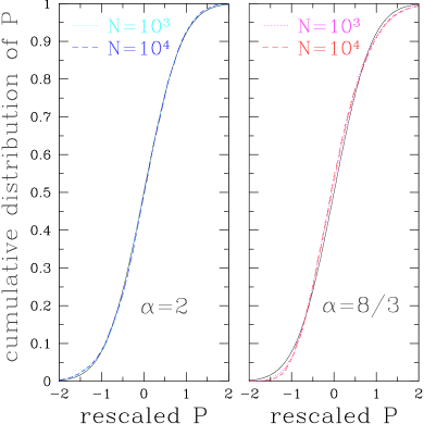
Figure 2: Numerical estimates for the cumulative probability distributions of the probability $P$ of success of the UC=R+UP algorithm on random 3-SAT instances with sizes $N=10^{3}$ (dots) and $10^{4}$ (dashes) and initial clauses-per-variable ratios $\alpha=2$ (left) and $8/3$ (right). The $P$-axis for each distribution (each value of $\alpha$ and $N$) is chosen so that the rescaled distributions have average 0 and standard deviation $1/\sqrt{2}$. The solid lines show the Gaussian cumulative distribution $[1+\mathrm{erf}(x)]/2$. For $\alpha=2$, numerical distribution are in good agreement with a Gaussian shape, but not for the critical ratio $\alpha=8/3$.

If we now plug the self-averaged form (19) of the $C_{j}$’s, $j\geq 2$, in their evolution equations (16), we get, using the reduced parameter $t=T/N$,

$$\frac{\mathrm{d}c_{j}}{\mathrm{d}t}=-\frac{j}{1-t}c_{j}(t)+\frac{j+1}{2(1-t)}c_{j+1}(t)\qquad\qquad 2\leq j\leq K$$ (27)

with $c_{K+1}:=0$. This triangular system of equations, with the initial conditions $c_{j}(0)=\alpha\delta_{j,K}$, is easily solved for given $K$. For instance, for $2+p$-SAT and the R heuristic, the solution reads

$$c_{3}(t) = \alpha p(1-t)^{3}$$ (28)

$$c_{2}(t) = \alpha(3pt/2+1-p)(1-t)^{2}$$ (29)

whereas, for $2+p$-SAT and the GUC heuristic,

$$c_{3}(t) = \alpha p(1-t)^{3}$$ (30)

$$c_{2}(t) = (1-t)\left\{\ln(1-t)+\alpha[3pt(2-t)/4+(1-p)]\right\}.$$

For K-SAT with the R heuristics with initial ratios $\alpha_{j}=C_{j}/N$,

$$c_{2}(t)=(1-t)^{2}\sum_{j=2}^{K}\alpha_{j}j(j-1)2^{1-j}t^{j-2}\ .$$ (32)

The parametric curve $[c_{2}(t),c_{3}(t),\ldots,c_{K}(t)]$, $0\leq t\leq 1$, will be called resolution trajectory. It describes, forgetting about 0- and 1-clauses, the typical evolution of the reduced formula under the operation of the algorithm. In the case of 3- or $2+p$-SAT, a useful alternative phase space is the $p\times\alpha$ plane, where $\alpha=(c_{2}+c_{3})/(1-t)$ is the (instantaneous) 2-or-3-clauses-per-variable ratio and $p$ is, as usual, the proportion of 3-clauses amongst the 2- and 3-clauses. Some resolution trajectories of the UC algorithm are shown on figure 3. They all end at the $c_{1}=c_{2}=c_{3}=0$ point with $t=1$: almost all variables have to be assigned before no clauses are left (and a solution is found). More clever algorithms such as GUC are able to find solutions with a finite fraction of remaining unset variables, and give a family of solutions with a finite entropy at once.

3.4 Reduced generating functions for 0- and 1-clause numbers

From now on, we identify $C_{2},C_{3},\ldots,C_{K}$ with their asymptotic averages $NC_{j}(t)$ as discussed above, and study the kinetics of $C_{0}$ and $C_{1}$ as driven by $C_{2},C_{3},\ldots,C_{K}$. Under these assumptions, it is easy to write the evolution equation for $C_{0}$ and $C_{1}$ that corresponds to (7): if $P(C_{0},C_{1};T|C_{2})$ is the probability that the search process leads, after $T$ assignments and with imposed values of $C_{2},C_{3},\ldots C_{K}$ at all steps 0 to $N$, to the numbers $C_{0}$, $C_{1}$ of 0-, 1-clauses,

$$P(C^{\prime}_{0},C^{\prime}_{1};T+1|C_{2})=$$ (33)

$$\qquad\sum_{C_{0}}\sum_{C_{1}}M_{1}[C^{\prime}_{0},C^{\prime}_{1}\leftarrow C_{0},C_{1};T|C_{2}]\ P(C_{0},C_{1};T|C_{2})$$

where the expression of $M_{1}$ is deduced from that of $M$ by canceling all what it written on the left of the sum over $z_{2}$ in (3.1). It is readily seen in that expression that, actually, the transition matrix $M_{1}$ doesn’t depend explicitly on $C_{3}$, $C_{4}$, …, $C_{K}$ but only on $C_{2}$; therefore, we dropped the unnecessary dependence in the above equation. $M_{1}$ also depends explicitly on time through $\mu=1/(N-T)$. This evolution equation translates into the following equation for the generating function

$$G_{01}(X_{0},X_{1};T|C_{2}):=\sum_{C_{0}=0}^{M}\sum_{C_{1}=0}^{M}\!\!X_{0}^{C_{0}}X_{1}^{C_{1}}P(C_{0},C_{1};T|C_{2}):$$

$$G_{01}(X_{0},X_{1};T+1|C_{2})=\left(1+\frac{X_{1}-1}{N-T}\right)^{C_{2}(\alpha,T)}\times$$ (34)

$$\ \left[\frac{1}{f_{1}}G_{01}(X_{0},f_{1};T|C_{2})+\left(1-\frac{1}{f_{1}}\right)G_{01}(X_{0},0;T|C_{2})\right]$$

where $f_{1}=\frac{1+X_{0}}{2(N-T)}+X_{1}(1-\frac{1}{N-T})$, see (12). Since the $X_{0}$ argument of $G_{01}$ is the same in all terms, we shall drop it when there is no ambiguity and use the lighter notation $G_{1}(X_{1};T|C_{2}):=G_{01}(X_{0},X_{1};T|C_{2})$. The key equation above yields the main results of the next Sections: in particular, $G_{01}(0,1;T|C_{2})$ is the probability that the search process detected no contradictions (i.e. produced no 0-clauses, even if there are already contradictory 1-clauses such as ‘$a$’ and ‘$\overline{a}$’) while assigning the first $T$ variables, and $G_{01}(0,1;T=N|C_{2})$ is the probability that a solution has been found by the search process, i.e. that all $N$ variables were assigned without production of a contradiction (if all variables were assigned, any produced contradiction was necessarily detected).

4 The probability of success

In this section, the generating function formalism is used to study the probability $P_{\mathrm{success}}(\alpha,p,N)$ that UC successfully finds a solution to a random instance of the $2+p$-SAT problem with $N$ variables and $\alpha N$ clauses. We first consider the infinite size limit, denoted by $P_{\mathrm{success}}(\alpha,p)$. As explained in Section 2.3, the probability of success vanishes everywhere but for ratios smaller than a critical value $\alpha_{\mathrm{R}}(p)$. This threshold line is re-derived, with a special emphasis on the critical behaviour of $P_{\mathrm{success}}$ when $\alpha\to\alpha_{\mathrm{R}}(p)$.

We then turn to the critical behaviour at large but finite $N$, with the aim of making precise the scaling of $P_{\mathrm{success}}(\alpha,p,N)$ with $N$. A detailed analysis of the behaviour of the terms appearing in the evolution equation for the generating functions $G$ (34) is performed. We show that the resulting scalings are largely common to all algorithms that use the Unit Propagation rule.

4.1 The infinite size limit, and the success regime

For a sufficiently low initial clauses-per-variables ratio $\alpha$, the algorithm finds a solution with positive probability when $N\to\infty$. It is natural to look for a solution of equation (34) with the following scaling:

$$G_{1}(X_{1},T=tN|C_{2})=\pi_{0}(X_{1},t)+o(1)$$ (35)

when $T,N\to+\infty$, $\pi_{0}$ being a smooth function of $X_{1}$ and $t$ ($X_{0}$ is kept fixed to 0). $\pi_{0}(1,t)$ is therefore, in the $N\to+\infty$ limit, the probability that the search process detected no contradiction after a fraction $t$ of the variable has been assigned. The probability of success we seek for is $P_{\mathrm{success}}=\pi_{0}(1,1)$.

We furthermore know that $C_{2}$, which drives the evolution of $C_{1}$ in (34), is concentrated around its average: we take

$$C_{2}(\alpha,T=tN)=(N-T)d_{2}(\alpha,t)+\mathcal{O}\left[(N-T)^{\delta}\right]$$ (36)

with

$$d_{2}(t):=c_{2}(t)/(1-t)$$ (37)

and $1/2<\delta<1$ will be chosen later. Inserting the above Ansätze into (34) yields

$$\pi_{0}(X_{1},t)=\frac{e^{(X_{1}-1)d_{2}(t)}}{X_{1}}\;\left[\pi_{0}(X_{1},t)+(X_{1}-1)\;\pi_{0}(0,t)\right]$$

$$\qquad+\mathcal{O}\left[(1-X_{1})(N-T)^{\delta-1}\right]+\mathcal{O}\left[(N-T)^{-1}\right]$$ (38)

hence, in the thermodynamic limit $N,T\to+\infty$, an equation for $\pi_{0}$,

$$\pi_{0}(X_{1},t)=\frac{e^{(X_{1}-1)d_{2}(t)}}{X_{1}}\;\left[\pi_{0}(X_{1},t)+(X_{1}-1)\;\pi_{0}(0,t)\right].$$ (39)

This equation does not suffice by itself to compute $\pi_{0}(1,t)$. Yet it yields two interesting results if we differentiate it w.r.t. $X_{1}$ to the first and second orders in $X_{1}=1$:

$$\pi_{0}(0,t) = \big{(}1-d_{2}(t)\big{)}\;\pi_{0}(1,t)$$ (40)

$$\frac{\partial\pi_{0}}{\partial X_{1}}(1,t) = \frac{d_{2}(t)\big{(}2-d_{2}(t)\big{)}}{2\big{(}1-d_{2}(t)\big{)}}\;\pi_{0}(1,t)\ .$$ (41)

Under assumption (35), $\pi_{0}(0,t)/\pi_{0}(1,t)=1-d_{2}(t)$ can be interpreted as the probability $\rho_{1}(t)$ that there is no 1-clause at time $t$ conditioned to the survival of the search process. $d_{2}(t)$ is then the (conditional) probability that there is at least one 1-clause . As $\rho_{1}(t)$ has to be positive or null, $d_{2}(t)$ cannot be larger than 1. As long as this is ensured, $\rho_{1}(t)$ has a well-defined and positive limit in the $N\to+\infty$ limit (at fixed reduced time $t$). The conditional average of $C_{1}$, $\partial_{X_{1}}\pi_{0}(1,t)/\pi_{0}(1,t)$, can be expressed from (41) and is of the order of one when $N\to+\infty$. The terms of the r.h.s. of (17) compensate each other: 1-clauses are produced from 2-clauses slower than they are eliminated, and do not accumulate. Conversely, in the failure regime (Sect. 2.3), 1-clauses accumulate, and cause contradictions.

To complete the computation of $\pi_{0}(1,t)$, we consider higher orders in the large $N$ expansion of $G_{1}$. In general, this would involve the cumbersome fluctuation term $\mathcal{O}\left[(X_{1}-1)(N-T)^{\delta-1}\right]$, but, at $X_{1}=1$, only the ‘deterministic’ $\mathcal{O}\left[(N-T)^{-1}\right]$ correction is left since $C_{2}$ disappears from equation (34). Thus we assume

$$G_{1}(1,T=tN|C_{2})=\pi_{0}(1,t)+\frac{1}{N-T}\;\pi_{1}(1,t)+o\left(\frac{1}{N-T}\right)$$ (42)

which yields, when inserted into (34),

$$-(1-t)\frac{\partial\pi_{0}}{\partial t}(1,t)=\frac{1}{2}\bigg{[}\frac{\partial\pi_{0}}{\partial X_{1}}(1,t)+\pi_{0}(0,t)-\pi_{0}(1,t)\bigg{]}\ .$$ (43)

This equation (43) can be turned into an ordinary differential equation for $\pi_{0}(1,t)$ using (40) and (41); after integrating over $t$, with the initial condition $\pi(1,t=0)=1$ i.e. no contradiction can arise prior to any variable setting, we find the central result of this section frieze-suen-guc-sc ; achlioptas-kirousis-kranakis-krizanc-2plusp-sat-rigoureux :

$$\pi_{0}(1,t)=\exp\left(-\int_{0}^{t}\frac{d\tau}{4(1-\tau)}\,\frac{d_{2}(\tau)^{2}}{1-d_{2}(\tau)}\right)$$ (44)

which is finite if, and only if, $d_{2}(\tau)<1$ for all $0\leq\tau\leq 1$ (the apparent divergence at $\tau=1$ is in practice compensated by the factors involving $d_{2}$).

The above result can be used in (40) and (39) to compute $\pi_{0}(X_{1},t)$, that is the generating function of the probability $P(C_{1},t)$ that there are $C_{1}$ 1-clauses and no contradiction has occurred after assignment of a fraction $t$ of the variables,

$$\pi_{0}(X_{1},t):=\sum_{C_{1}\geq 0}P(C_{1},t)\;X_{1}^{C_{1}}$$

$$\qquad=[1-d_{2}(t)]\,\frac{1-X_{1}}{1-X_{1}e^{-(X_{1}-1)d_{2}(t)}}\;\pi_{0}(1,t).\quad$$ (45)

As long as $d_{2}(t)<1$, the average number of 1-clauses $\langle C_{1}\rangle(t)$ is finite as $N\to+\infty$. This sheds light on the finiteness of $P_{\mathrm{success}}$. The probability of not detecting a contradiction at the time step $T\to T+1$ is $(1-\mu/2)^{\max(C_{1}-1,0)}\simeq 1-\max(C_{1}-1,0)/2/(N-T)$, and $P_{\mathrm{success}}$ is the product of $\Theta(N)$ quantities of that order .

The validity condition $d_{2}(t)=c_{2}(t)/(1-t)<1$ is fulfilled at all steps $t$ if, and only if, the initial clauses-per-variable ratio $\alpha$ is smaller than a threshold, $\alpha_{\mathrm{R}}$, as can be seen from the expression of $c_{2}(t)=\langle C_{2}\rangle(T)/N$ that results from equation (29). Graphically, in the $(p,\alpha)$ plane, the resolution trajectory in Figure 3 stays below the line $\alpha(1-p)=1$ iff. $\alpha$ is small enough. Finding the threshold value for $\alpha$ and a given $p$ is an easy ballistic problem:

• If $p<2/5$ (‘2-SAT family’), whatever the initial clauses-per-variable $\alpha$, the resolution trajectory (figure 3) will always either be entirely below the $d_{2}=1$ line (success case, low $\alpha$), or cut it (failure case, high $\alpha$). The threshold value of $\alpha$ is reached when the resolution trajectory starts exactly on it (critical case), therefore

  $$\alpha_{\mathrm{R}}(p)=1/(1-p)\quad\text{if }p<2/5.$$ (46)

• If $p\geq 2/5$ (‘3-SAT class’), the resolution trajectory for low $\alpha$ is also entirely below the $d_{2}=1$ line (success case). This situation ends when the resolution trajectory gets tangent to the $d_{2}=1$ line, whereas for $p<2/5$ it was secant. All critical trajectories for $p\geq 2/5$ share the support of the critical trajectory for $p=1$ (3-SAT) that starts at $(p=1,\alpha=8/3)$, and all become tangent to the $d_{2}=1$ line at the $(p=2/5,\alpha=5/3)$ point (reached after a finite time), whereas for $p<2/5$ there are several critical trajectories. Here,

  $$\alpha_{\mathrm{R}}(p)=24p/(2+p)^{2}\quad\text{if }p\geq 2/5.$$ (47)

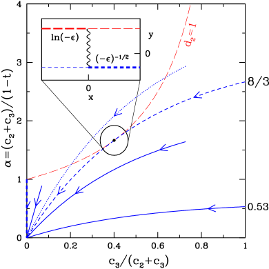
Figure 3: Some resolution trajectories of the UC=UP+R algorithm. If the trajectory of some algorithm stays strictly below the $d_{2}=\alpha(1-p)=1$ line (long-dashed line), 1-clauses don’t accumulate and the success probability $P_{\mathrm{success}}$ of the algorithm is finite as $N\to+\infty$ (solid trajectories). Critical behaviour is when the trajectory gets tangent to this line or starts on it (short-dashed trajectories). When the trajectory spends time in the region above this line (dotted trajectory), $P_{\mathrm{success}}$ gets exponentially small in $N$. Inset: The singular behaviour of $P_{\mathrm{success}}$ around the $(p=2/5,\alpha=5/3)$ point is better understood if one uses local coordinates $(x,y)$. $x$ is the distance along the common tangent to the $d_{2}=1$ line and the critical trajectory. $y$ is such that lines of constant $y$ are, in the original coordinates, parabolas, tangent to the $d_{2}=1$ line. The point $(2/5,5/3)$ is spread onto the waved line. Left and right limits of $P_{\mathrm{success}}$ for $x\to 0$ on the waved line are well-defined but distinct. The $N\to+\infty$ limit of $-\ln P_{\mathrm{success}}$ has the indicated singularities on the thick lines.

The probability $P_{\mathrm{success}}=\pi_{0}(1,1)$ that the UC algorithm finds a solution is obtained from equation (44) with $d_{2}(t)=\alpha(1-t)(3/2pt+1-p)$, equation (29):

$$-\ln P_{\mathrm{success}}(\alpha,p)=\frac{1}{4\sqrt{24p/(2+p)^{2}/\alpha-1}}\times$$ (48)

$$\qquad\left[\mathrm{arctan}\frac{1}{\sqrt{24p/(2+p)^{2}/\alpha-1}}+\right.$$

$$\qquad\left.\ \,\mathrm{arctan}\frac{5(p-2/5)}{(2+p)\sqrt{24p/(2+p)^{2}/\alpha-1}}\right]$$

$$\qquad-\frac{1}{8}\ln\left(\frac{1}{1-p}-\alpha\right)-\frac{1}{8}\ln(1-p)+\frac{\alpha(p-4)}{16}\ .$$

Of particular interest is the singularity of $P_{\mathrm{success}}$ slightly below the threshold ratio. At fixed $p$, as $\alpha$ increases, the first singularity is encountered when the resolution trajectory tangent to the $d_{2}=1$ line is crossed i.e. for $\alpha=24p/(2+p)^{2}$ (figure 3, largest short-dashed line, and thick short-dashed line in the inset). If $p>2/5$ (3-SAT class), the two $\mathrm{arctan}$ in equation (48) tend to $\pi/2$ and $P_{\mathrm{success}}$ vanishes as ($\epsilon<0$):

$$-\ln P_{\mathrm{success}}\left[(1+\epsilon)\alpha_{\mathrm{R}}(p),p\right]=\frac{\pi}{4}\frac{1}{\sqrt{-\epsilon}}+\Theta(1).$$ (49)

For $p=2/5$, one of the two $\mathrm{arctan}$ vanishes for all $\alpha$, and the first $\ln$ brings another singularity ($\epsilon<0$):

$$-\ln P_{\mathrm{success}}\left[\frac{5}{3}(1+\epsilon),\frac{2}{5}\right]=\frac{\pi}{8}\frac{1}{\sqrt{-\epsilon}}-\frac{1}{8}\ln(-\epsilon)+\Theta(1).$$ (50)

And for $p<2/5$, the two $\mathrm{arctan}$ have opposite signs so that the first term of equation (48) has no singularity while crossing the ‘limiting’ resolution trajectory $\alpha=24p/(2+p)^{2}$ (thin short-dashed line of the inset of Fig. 3). A singularity is found when $\alpha$ reaches the $d_{2}=1$ line, $\alpha=1/(1-p)$ (thick long-dashed line of the inset of figure 3), with the outcome ($\epsilon<0$)

$$-\ln P_{\mathrm{success}}\left[(1+\epsilon)\alpha_{\mathrm{R}}(p),p\,\right]=-\frac{1-p}{2(2-5p)}\ln(-\epsilon)+\Theta(1).$$ (51)

The difference of nature of the singularities between the 2-SAT and 3-SAT families corresponds to different divergences of $-\ln P_{\mathrm{success}}$ with $N$, as will be computed in the next section.

For completeness, let us check that the above calculation is compatible with our approximation (3.3). The first term of the l.h.s. there is equal to $P_{\mathrm{success}}$ plus the $1/(N-T)$ correction from equation (42). The second term there, in $\mathcal{O}(N^{\zeta})$, corresponds here to the fluctuations of $C_{2}$: $\mathcal{O}(N^{\delta-1})$ in equation (4.1), thus $\zeta=\delta-1$. If we take for $\delta$ any value on the allowed interval $]1/2,1[$, the two approximation terms in (3.3) vanish as $N\to+\infty$. Therefore, as long as $P_{\mathrm{success}}$ is finite for large $N$, these approximation terms are actually negligible.

4.2 Large $N$ scalings in the critical regime

Our previous study of the success regime breaks down when $d_{2}(t)$ reaches 1 during operation of the algorithm. Indeed, consider the infinite-$N$ generating function for $C_{1}$, $G_{1}$, given by eq. (4.1). As a function of $X_{1}$, $G_{1}$ vanishes uniformly on any compact interval $[0,1-\eta]$, $\eta>0$, as $d_{2}\to 1$. The $X_{1}=1$ point is singular since normalization enforces $\pi_{0}(1,t)=1$ (assuming $X_{0}=1$): all useful information is concentrated in a small region around $X_{1}=1$. Expanding eq. (4.1) for $X_{1}\to 1$ yields

$$\pi_{0}(X_{1},t) = \left\{1+d_{2}(t)\frac{1-X_{1}}{1-d_{2}(t)}-\frac{X_{1}d_{2}^{2}(t)}{2}\frac{1-X_{1}}{1-d_{2}(t)}+\right.$$ (52)

$$\left.\ \,\mathcal{O}\left[\frac{(1-X_{1})^{2}}{1-d_{2}(t)}\right]\right\}^{-1}.$$

Non-trivial results are obtained when $1-X_{1}$ and $1-d_{2}(t)$ are of the same (vanishingly small) order of magnitude — let us call it $\Delta$. We suspect that $\Delta$ is some negative power of $N$, to be determined below. Let us define

$$X_{1}=:1-x_{1}\Delta,\quad e_{2}(t):=\Delta^{-1}(1-d_{2}(t))$$ (53)

so that eq. (36) now reads

$$C_{2}[\alpha,T=tN]=[1-e_{2}(\alpha,t)\Delta](N-T)+\mathcal{O}\left[(N-T)^{\delta}\right]$$ (54)

where, as previously, the exponent $\delta$ will be tuned later according to the framework eq. (3.3).

We assume that, in the thermodynamic limit $N\to\infty,\Delta\to 0$ but at fixed $x_{1}$, $e_{2}(t)$, and time $t$, the normalized generating function of $C_{1}$ conditioned to the typical value of $C_{2}(t)$,

$$\frac{G_{1}(X_{1}=1-x_{1}\Delta,T=tN|C_{2})}{G_{1}(1,T=tN|C_{2})}\,\mathop{\relbar\joinrel\relbar\joinrel\relbar\joinrel\relbar\joinrel\rightarrow}_{N\to+\infty}\overline{\pi}(x_{1},t)$$ (55)

where the limit $\overline{\pi}$ is a smooth function of $x_{1}$ and $t$ (which also depends on $X_{0}$ and $e_{0}$). $\overline{\pi}(x_{1},t)$ is the generating function for the stochastic variable $c:=C_{1}/\Delta$, conditioned to the success of the algorithm. Eq. (52) gives information about the $e_{2}\to+\infty$ limit of $\overline{\pi}$. Furthermore, eq. (4.1) shows that

$$\Delta^{-1}G_{1}(0,T|C_{2})/G_{1}(1,T|C_{2})\,\mathop{\relbar\joinrel\relbar\joinrel\relbar\joinrel\relbar\joinrel\rightarrow}_{N\to+\infty}\sigma(t)\ ,$$ (56)

a well defined limit of the order of unity for $T=tN$ and $C_{2}$ given by eq. (54). We now plug the previous conventions and assumption into the evolution equation for the conditional, normalized generating function of $C_{1}$. This equation is formed by dividing eq. (34) by $G_{1}(1,T|C_{2})$, which yields, in a formal way,

$$\mathrm{LHS} = \mathrm{RHS}_{1}+\mathrm{RHS}_{2}$$ (57)

$$\mathrm{LHS} := G_{1}(X_{1},T+1|C_{2})/G_{1}(1,T|C_{2})$$

$$\mathrm{RHS}_{1} := \left(1+\frac{X_{1}-1}{N-T}\right)^{C_{2}(\alpha,T)}\frac{1}{f_{1}}\frac{G_{1}(f_{1};T|C_{2})}{G_{1}(1,T|C_{2})}$$

$$\mathrm{RHS}_{2} := \left(1+\frac{X_{1}-1}{N-T}\right)^{C_{2}(\alpha,T)}\left(1-\frac{1}{f_{1}}\right)\frac{G_{1}(0;T|C_{2})}{G_{1}(1,T|C_{2})}\ .$$

From this equation we get, in the following subsections, all results relevant to the critical behaviour of the success probability of the greedy algorithm.

4.2.1 Analysis of the RHS terms

The two contributions of the r.h.s. of the evolution equation (57) have the detailed expression (for $X_{0}=0$):

$$\mathrm{RHS}_{1} = \left\{1+x_{1}e_{2}(t)\Delta^{2}+\frac{1}{2N(1-t)}+\frac{x_{1}^{2}}{2}\Delta^{2}+\right.$$ (58)

$$\ \mathcal{O}((x_{1}^{3}+x_{1}^{2}e_{2}(t))\Delta^{3})+\mathcal{O}(x_{1}\frac{\Delta}{N(1-t)})+$$

$$\ \mathcal{O}\left[x_{1}\Delta(N-T)^{\delta-1}\right]\bigg{\}}\times$$

$$\left\{\overline{\pi}(x_{1},t)+\frac{1}{2N(1-t)\Delta}\partial_{x_{1}}\overline{\pi}(x_{1},t)+\right.$$

$$\ \,\mathcal{O}\left[(N-T)^{-2}\Delta^{-2}\right]\bigg{\}}\quad$$

and

$$\mathrm{RHS}_{2}=-\sigma(t)\Delta\left\{x_{1}\Delta+\frac{1}{2N(1-t)}+\mathcal{O}(\frac{x_{1}\Delta}{N(1-t)})+\right.$$

$$\quad\mathcal{O}(x_{1}^{3}\Delta^{3})+\mathcal{O}\left[(N-T)^{-2}\right]+\mathcal{O}\left\{x_{1}^{2}\Delta^{2}(N-T)^{\delta-1}\right]\bigg{\}}$$

where, as usual, $T=tN$.

Apart from the dominant term $\overline{\pi}(x_{1},t)$ that cancels with the dominant term of the l.h.s., the first terms have order $\Delta^{2}$ and $1/(N\Delta)$ (we here assume that $t<1$ in the critical regime, which will be the case in all subsequent situations). Then, $\Delta^{3}$, $1/N$, $\Delta/N$ and so on are negligible for large $N$ (because $\Delta$ vanishes, but slower than $1/(N-T)$ since the integer $C_{2}$ may not vary by less than unity). So do the terms stemming from fluctuations of $C_{2}$ around its typical value, $\Delta^{2}(N-T)^{\delta-1}$ and $\Delta(N-T)^{\delta-1}$, if we choose $\delta$ carefully (see below). Choosing $\Delta$ such that $\Delta^{2}=1/(N\Delta)$ allows us to gather a maximal number of terms in the equation for $\overline{\pi}$. Other choices are possible but trivial, in that they would correspond to either the success or the failure regimes, but not to the critical case. From now on, $\Delta:=N^{-1/3}$.

Then, the fluctuations of $C_{2}$ in the above expansion are of the order of $\Delta(N-T)^{\delta-1}=(N-T)^{\delta-4/3}$. Using the notations from eq. (3.3), $\zeta=\delta-4/3$. These fluctuations are negligible with respect to $N^{2/3}$ if $\delta<2/3$. Remember that the range of possible values for $\delta$ was $]1/2,1[$; in the critical situation here, we may choose $\delta\in]1/2,2/3[$. It will be checked later that the third term of the l.h.s. of eq. (3.3) is also negligible w.r.t. the first one. Finally,

$$\mathrm{RHS}_{1}+\mathrm{RHS}_{2}=\overline{\pi}(x_{1},t)+N^{-2/3}\times$$

$$\quad\left[\frac{1}{2(1-t)}\partial_{x_{1}}\overline{\pi}(x_{1},t)+\big{(}e_{2}(t)\;x_{1}+\frac{x_{1}^{2}}{2}\big{)}\overline{\pi}(x_{1},t)\right.$$

$$\quad\ \,-\sigma(t)x_{1}\bigg{]}+\mathcal{O}\left[(N-T)^{-1},x_{1}(N-T)^{\delta-4/3}\right].$$ (59)

4.2.2 Analysis of the LHS terms

LHS in eq. (57) has to do with time evolution. The values of $d_{2}$ or $e_{2}$ are given by the average value of $C_{2}$ calculated in Section 3.3. $e_{2}$ is of the order of unity when $N\to+\infty$ if the resolution trajectory comes close to $d_{2}=1$ i.e. if the initial clauses-per-variable ratio $\alpha$ is close to its threshold value eqs. (46 - 47). We zoom in around the time, say, $t^{*}$ where $d_{2}$ is closest to 1 (or equal to 1 if we are exactly on the borderline between the success and failure cases) and let

$$T=t^{*}\,N+t_{0}N\Delta^{a}=t^{*}\,N+t_{0}N^{1-a/3}.$$ (60)

$a$ will be fixed later for each family of near-critical trajectories so that $1-d_{2}(t)$ is indeed of order $\Delta$ on a finite interval of rescaled times $t_{0}$. We now assume that $\overline{\pi}$ and $G_{1}(X_{1}=1)$ have, when $N\to\infty$ and time $T$ is given by (60), well defined limits, regular w.r.t. $t_{0}$ . The l.h.s. of eq. (57) may be written for large $N$

$$\mathrm{LHS}=G_{1}(1,T+1|C_{2})/G_{1}(1,T|C_{2})\ \overline{\pi}(x_{1},T+1)$$ (61)

where $T+1=t_{0}+N^{-1}\Delta^{-a}=t_{0}+N^{-1+a/3}$. As time $t_{0}$ goes on, the shape of the distribution of $C_{1}/\Delta$ (encoded into $\overline{\pi}$) and the probability of success (given by $G_{1}(1,T|C_{2})$) both vary. Fix first $x_{1}$ at 0 so that $X_{1}=1$ and $\overline{\pi}=1$, then eqs. (61) and (4.2.1) read

$$\mathrm{LHS} = 1+N^{-1+a/3}\partial_{t_{0}}\ln[G_{1}(1,t_{0}|C_{2})]$$ (62)

$$\mathrm{RHS}_{1}+\mathrm{RHS}_{2} = 1+\frac{1}{2(1-t)}N^{-2/3}\partial_{x_{1}}\overline{\pi}(1,t)+$$ (63)

$$\mathcal{O}\left[(N-T)^{-1}\right].$$

Comparing the two members, eq. (62) and eq. (63), of eq. (57) shows that $\ln[G_{1}(1,t_{0}|C_{2})]$ is of the order of $N^{(1-a)/3}$, with subleading terms of the order of $N^{-a/3}$ at most. Defining $\lambda:=(1-a)/3$, we have in the large $N$ limit

$$-N^{-\lambda}\ln G_{1}(1,T|C_{2})\to\mu(t_{0}),$$ (64)

a regular function of $t_{0}$. Eqs. (62) and (4.2.1) with $x_{1}=0$ yield

$$\partial_{t_{0}}\mu(t_{0})=-\frac{1}{2(1-t^{*})}\partial_{x_{1}}\overline{\pi}(0,t_{0}).$$ (65)

As $\overline{\pi}$ is the generating function of $c=C_{1}/\Delta$ (conditioned to success of the algorithm),

$$\overline{c}(t_{0}):=-\partial_{x_{1}}\overline{\pi}(0,t_{0})$$ (66)

is the conditional average of the rescaled number $c$ of unit-clauses.

For general $x_{1}$ now, the previous assumptions lead from the expression (61) of the l.h.s. of eq. (57) to

$$\mathrm{LHS} = \overline{\pi}(x_{1},t_{0})+N^{-1+a/3}\partial_{t_{0}}\overline{\pi}(x_{1},t_{0})$$ (67)

$$-N^{-2/3}\overline{\pi}(x_{1},t_{0})\partial_{t_{0}}\mu(t_{0})+\mathcal{O}(N^{-2+2a/3}).\quad$$

4.3 Critical evolution equations

Comparing the two sides of the evolution equation, eq. (4.2.1) and eq. (67), we are left with two situations.

• If $a=1$: $\lambda=0$ and it is convenient to use the non-normalized (non-conditional) generating function

  $$\pi(x_{1},t_{0}):=\exp[-\mu(t_{0})]\overline{\pi}(x_{1},t_{0}).$$

  The total probability here, $\pi(0,t_{0})$, is not 1 as for $\overline{\pi}$ but the success probability of the greedy algorithm. $\pi$ satisfies the following PDE:

  $$\partial_{t_{0}}\pi(x_{1},t_{0}) = \frac{1}{2(1-t^{*})}\partial_{x_{1}}\pi(x_{1},t_{0})+$$

  $$\left[e_{2}(t_{0})x_{1}+\frac{x_{1}^{2}}{2}\right]\pi(x_{1},t_{0})-\sigma(t_{0})x_{1}.$$

• If $a<1$: the probability of success has the scaling relationship $P_{\mathrm{success}}\propto\exp[-\Theta(N^{(1-a)/3})]$. The time-derivative term $\partial_{t_{0}}\overline{\pi}(x_{1},t_{0})$ is negligible w.r.t. other terms, and $\overline{\pi}$ satisfies the ODE:

  $$0 = \frac{1}{2(1-t^{*})}\left[\partial_{x_{1}}\overline{\pi}(x_{1},t_{0})+\overline{c}(t_{0})\overline{\pi}(x_{1},t_{0})\right]+$$ (69)

  $$\left[e_{2}(t_{0})x_{1}+\frac{x_{1}^{2}}{2}\right]\overline{\pi}(x_{1},t_{0})-\sigma(t_{0})x_{1}\ .$$

The third possibility, $a>1$, leads to inconsistencies and has to be rejected .

In the previous section, we classified the critical resolution trajectories into two families: those of the 2-SAT family ($p<2/5$) start from the $d_{2}=1$ line but are secant to it, and those of the 3-SAT family ($p>2/5$) do not start on this line but get tangent to it (‘parabola situation’). As we will see in the next sections, these two families correspond, respectively, to values of the exponent $a$ equal to 1 and $1/2$, making successively eq. (• ‣ 4.3) and (69) relevant.

5 The 2-SAT class (power law class)

5.1 Equations for 2-SAT and its family

When $p<2/5$, the critical resolution trajectory starts on the $d_{2}=1$ line and is secant to it (at time $t^{*}=0$) with slope

$$\beta(p):=\frac{2-5p}{2(1-p)}.$$ (70)

The threshold value of $\alpha$ is $\alpha_{\mathrm{R}}(p)=1/(1-p)$ (eq. 46). On this resolution trajectory, $1-d_{2}(t-t^{*})\propto t-t^{*}$. Therefore, this resolution trajectory is at distance $\Delta=N^{-1/3}$ of the $d_{2}=1$ line as long as $t-t^{*}$ is of order $\Delta^{1}$: the exponent $a$ equals 1 here and the relevant equation is eq. (• ‣ 4.3).

The critical regime is realized when $\alpha$ is close to the value $\alpha_{\mathrm{R}}(p)=1/(1-p)$. The relevant scaling is

$$\alpha=\alpha_{\mathrm{R}}(p)(1+\epsilon_{\alpha}N^{-1/3})$$ (71)

with finite $\epsilon_{\alpha}$ since, if $\alpha$ is less than $\alpha_{\mathrm{R}}(p)$ by more than $\Delta=N^{-1/3}$, at the initial date $t=0$, $d_{2}(0)$ is already out of the critical region $1-\Delta$ (remember that $d_{2}(t)$ decreases with time if $p<2/5$ as can be seen in Fig. 3). Conversely, if $\alpha$ is above $\alpha_{\mathrm{R}}(p)$ by a distance much greater than $\Delta$ at time $t=0$, $1-d_{2}(0)$ is an order of magnitude higher than the critical distance $\Delta$ and an infinite duration, on the scale of $t_{2}$ in eq. (60) with $a=1$, is needed until this critical distance is reached. Notice that the critical window here coincides with the critical window of the static phase transition for 2-SAT bollobas-borgs-chayes-2sat-scaling-window . remember, deals with the mere existence of satisfying rather than with the ability of some algorithm to find them)

Finally, $t^{*}$ is such that $d_{2}(t)=1$, therefore

$$t^{*}=\epsilon_{\alpha}/\beta(p)N^{-1/3}+\mathcal{O}(N^{-2/3})$$

from eq. (29), and the relevant scaling for time is

$$T=\left[t_{2}+\epsilon_{\alpha}/\beta(p)\right]N^{2/3}$$ (72)

according to eq. (60), where we replaced the notation $t_{0}$ with $t_{2}$ to emphasize that this scaling is proper to the 2-SAT family.

We have to solve eq. (• ‣ 4.3) with this choice of scales and with proper initial and boundary conditions. Define

$$p_{\mathrm{no-contr}}(\to t_{2}):=\pi(x_{1}=0,t_{2}).$$ (73)

This is the probability that the algorithm detects no contradiction from $T=0$ up to the (rescaled) time $t_{2}$. We shall send $t_{2}\to+\infty$ at the end. In the case of the greedy UC algorithm, $1/[2(1-t^{*})]=1/2+\mathcal{O}(N^{-1/3})$ and $e_{2}(t_{2})=\beta(p)t_{2}+\mathcal{O}(N^{-1/3})$, so that eq. (• ‣ 4.3) reads:

$$\partial_{t_{2}}\pi(x_{1},t_{2})=\frac{1}{2}\partial_{x_{1}}\pi(x_{1},t_{2})+$$

$$\qquad\left[\beta(p)t_{2}x_{1}+\frac{x_{1}^{2}}{2}\right]\pi(x_{1},t_{2})-\sigma(t_{2})x_{1}.$$ (74)

In practice, we find it easier to perform an inverse Laplace transform of eq. (• ‣ 4.3) before solving it; this amounts to work with probability density functions (PDFs) rather than with generating functions. In particular, the difficulty of computing $\sigma$ that appears in eq. (• ‣ 4.3) is turned into a boundary condition on the PDF that is easier to deal with.

If we plug the critical scaling of $X_{1}$, eq. (53), into the definition of the generating function $G_{1}(X_{1})$ of $C_{1}$:

$$G_{1}(X_{1}) := \sum_{C_{1}=0}^{+\infty}X_{1}^{C_{1}}P(C_{1})$$ (75)

$$= \sum_{C_{1}=0}^{+\infty}e^{-x_{1}C_{1}N^{-1/3}+\mathcal{O}(N^{-2/3})}P(C_{1})$$

and (in an heuristic way) change the discrete sum on $C_{1}$ into an integral on $c:=C_{1}N^{-1/3}$, letting $N$ go to $+\infty$:

$$\pi(x_{1})=\int_{0}^{+\infty}e^{-x_{1}c}\rho(c)\,\mathrm{d}c$$ (76)

where $\rho(c)$ is the probability density function (PDF) of $c$, we see that $\pi(x_{1})$ is the Laplace transform of $\rho(c)$ with respect to $c$. Here we have dropped the time dependence, but $\rho(c,t_{2})$ is actually a function of $c$ and $t_{2}$ and the Laplace transform is taken at fixed time.

In terms of $\rho(c,t_{2})$, eq. (5.1) translates into

$$\partial_{t_{2}}\rho(c,t_{2})=\frac{1}{2}\partial_{c}^{2}\rho(c,t_{2})+\beta(p)\;t_{2}\;\partial_{c}\rho(c,t_{2})-\frac{1}{2}c\;\rho(c,t_{2})\ .$$ (77)

This inverse Laplace transform can be performed only if the limit when $x_{1}\to+\infty$ of the r.h.s. of eq. (5.1) is zero. Writing from (76) the asymptotic expansion for $\pi(x_{1},t_{2})$ in terms of the density of clauses and its derivatives at the origin $c=0$,

$$\pi(x_{1},t_{2})=\rho(0,t_{2})/x_{1}+\partial_{c}\rho(0,t_{2})/x_{1}^{2}+o(1/x_{1}^{2})$$ (78)

and plugging it into eq. (5.1), we find that $\sigma(t_{2})=1/2\;\rho(0,t_{2})$ and $\rho(c,t_{2})$ satisfies the boundary condition:

$$\frac{1}{2}\partial_{c}\rho(0,t_{2})+\beta(p)\;t_{2}\;\rho(0,t_{2})=0.$$ (79)

Conversely, one verifies that eq. (77) supplemented with the boundary condition eq. (79) leads by direct Laplace transform to eq. (5.1) where $\sigma(t_{2})$ is replaced with $\rho(0,t_{2})/2$.

Eq. (77), supplemented with eq. (79), is a reaction-diffusion equation on the semi-infinite axis of $c=C_{1}/(N-T)^{1/3}>0$. At the initial time step $T=0$, i.e. $t_{2\mathrm{init}}=-\epsilon_{\alpha}/\beta(p)$, there are no 1-clauses, so that $\pi(x_{1},t_{2\mathrm{init}})=1$ for all $x_{1}$ and $\rho(c,t_{2\mathrm{init}})$ is a Dirac $\delta$ distribution centered on $c=0$: the diffusing particles all sit on the $c=0$ point. Then, they start diffusing (second-derivative term in Eq. (77)) because new 1-clauses are produced randomly from 2-clauses when variables are assigned by the algorithm. This diffusion is biased: the drift term $\partial_{c}\rho(c,t_{2})$ comes from the tendency of the algorithm to make 1-clauses disappear (to satisfy them). A picture of this process may be found in the upper-right inset of Figure 8, where the PDF $\rho$ is shown after normalization. The total number of particles is not conserved: the absorption term $c\rho(c,t_{2})$ results from the stopping of some runs of the algorithm, those where a contradiction (a 0-clause) is detected. The probability that no contradiction has been encountered till time $t_{2}$, $p_{\mathrm{no-contr}}(\to t_{2})=\pi(0,t_{2})=\linebreak\int_{c=0}^{+\infty}\rho(c,t_{2})\mathrm{d}c$, is a decreasing function of $t_{2}$, smaller than unity.

5.2 Results for 2-SAT and its family

Unfortunately, we were not able to solve analytically eq. (77). Our study relies on an asymptotic expansion of the solution of this equation for large times $t_{2}$ and on a numerical resolution procedure to get results at finite times $t_{2}$. This numerical resolution was in turn helped with an asymptotic expansion at small times $t_{2}$.

Details about the large times $t_{2}$ expansion may be found in Appendix C. In short, we find that the probability that the greedy algorithm does not stop till time $t_{2}$ decays algebraically at large times,

$$p_{\mathrm{no-contr}}(\to t_{2})=\int_{0}^{+\infty}\rho(c,t_{2})\mathrm{d}c\quad\propto\quad t_{2}^{-\frac{1}{4\beta}}\ .$$ (80)

The leading order of the probability of success at the final time step $T=N$ can be guessed by replacing $t_{2}$ with $N^{1/3}$:

$$P_{\mathrm{success}}[\alpha_{\mathrm{R}}(p),p]\propto N^{-\frac{1}{12\beta}}\ ,$$ (81)

an intermediate behaviour between the success (finite $P_{\mathrm{success}}$) and failure ($-\ln P_{\mathrm{success}}\propto N$) situations defined in Section 2.3.

The proportionality factor in eq. (81) can be calculated through a numerical resolution of eq. (77) for finite values of $t_{2}$.

5.2.1 Numerical resolution of eq. (77) at finite times $t_{2}$

We have solved the reaction-diffusion-like eq. (77) thanks to a standard numerical resolution scheme (the Crank-Nicholson method) after some preliminary steps. First we discretized both time and ‘space’ (the semi-infinite axis of $c$). It is convenient to consider finite-support functions, and we have tried the changes of variables $b=1/(c+1)$ and $b=\exp(-c)$; the latter turned out to be better. The range $]0,1]$ for $b$ was discretized into $\mathcal{N}$ points. The Crank-Nicholson method allows us to take a time step $1/\mathcal{N}$ for the numerical resolution (quite efficient as compared to the time step $1/\mathcal{N}^{2}$ for Euler’s method), provided that the Courant condition is respected. With eq. (77) this is not the case, since the coefficient of the drift term, $\beta(p)t_{2}$, is not bounded with growing $t_{2}$. We actually consider $\tilde{\rho}(c,t_{2})=\exp(-\beta ct_{2}-\beta^{2}t_{2}^{3}/6)\rho(c,t_{2})$ rather than $\rho(c,t_{2})$ so that the Courant condition is satisfied. What we have to solve now is

$$\partial_{t_{2}}\tilde{\rho}(b,t_{2})=\frac{b^{2}}{2}\partial_{b}^{2}\tilde{\rho}(b,t_{2})+\frac{b}{2}\partial_{b}\tilde{\rho}(b,t_{2})$$

$$\qquad\quad-\left[\beta(p)-\frac{1-X_{0}}{2}\right]\ln(b)\tilde{\rho}(b,t_{2})$$ (82)

with $X_{0}=0$ and for $0<b\leq 1$, and with the boundary condition

$$\partial_{b}\tilde{\rho}(1,t_{2})-\beta(p)t_{2}\tilde{\rho}(1,t_{2})=0\ .$$ (83)

At initial time ${t_{2}}_{\mathrm{init}}=-\epsilon_{\alpha}/\beta(p)$, $\rho(c,{t_{2}}_{\mathrm{init}})=\delta(c)$. The most relevant term in eq. (77) is the diffusion term, and we expect $c$ to grow like $\sqrt{t_{2}-{t_{2}}_{\mathrm{init}}}$ typically . Therefore, we start our numerical resolution at time ${t_{2}}_{\mathrm{init}}+\mathcal{N}^{-1/2}$ so that a finite number of discretization points (instead of just the point on the $b=1$ boundary) share the support of $\tilde{\rho}$. The initial condition is given by a short-time series expansion of the solution of eq. (77). Details about this expansion are found in Appendix D.

We first tested our program by studying the linear equation eq. (77), or more precisely eq. (5.2.1) with $X_{0}$ set to 1. In this case, the distribution $\rho$ is normalized to unity. We observed that this conservation rule is fulfilled by our numerical resolution scheme up to a small deviation of order $1/\mathcal{N}$, diverging with the simulation time $t_{2}$. Therefore, we must be careful in our choice for the final time of the simulation. Moreover, when we plotted the conditional average $\overline{c}(t_{2})$, we found a very good agreement with the analytical expansions at small and large times $t_{2}$. This agreement was also observed for the non-linear equation eq. (5.2.1) — see Figure 4. Therefore, we think that our numerical results are quite reliable, at least on finite time ranges.

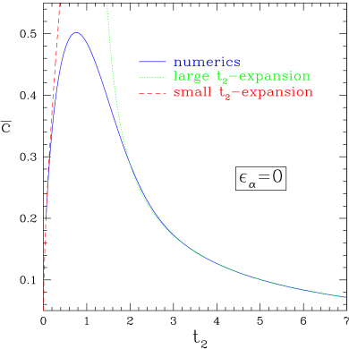
Figure 4: Numerical data for $\overline{c}(t_{2})$ in the case of critical 2-SAT ($\beta=1$ and $\epsilon_{\alpha}=0$), obtained by numerically solving eq. (77). Comparisons with the analytical small- and large-times asymptotic expansions are shown.

5.2.2 Probability of success in the critical time regime and the scaling function $H$

As the numerical precision on $\overline{c}(t_{2})$ is greater than on the total probability , we have calculated the probability of success through the numerical results for $\overline{c}$. The probability $\overline{\pi}(0,t_{2})$ is indeed related to the values of $\overline{c}(t_{2})$ by integrating eq. (77) over $c$ from 0 to $+\infty$, see eq. (65):

$$\partial_{t_{2}}\ln p_{\mathrm{no-contr}}(\to t_{2})=-\overline{c}(t_{2})/2$$ (84)

where we have used the boundary condition eq. (79). In practice, we integrated $\overline{c}$ numerically from $t_{2\mathrm{init}}$ (which depends on $p$ and $\epsilon_{\alpha}$) to $t_{2}\approx 5$, and used our large-$t_{2}$ expansion (see Eq. (80) and Appendix C) for $t_{2}>5$, which yields

$$-\ln p_{\mathrm{no-contr}}(\to t_{2};\epsilon_{\alpha},p)=\frac{\ln t_{2}}{4\beta(p)}+H[\epsilon_{\alpha},\beta(p)]+\mathcal{O}\left(t_{2}^{-3}\right)$$ (85)

with the following values for $H$ at criticality ($\epsilon_{\alpha}=0$): $0.24371\pm 10^{-5}$ for $p=0$, $0.24752\pm 10^{-5}$ for $p=1/7$, $0.20157\pm 10^{-5}$ for $p=1/4$, $-0.208\pm 10^{-3}$ for $p=1/3$. These values are extrapolations to $\mathcal{N}=\infty$ of numerical results for a number of discretization points $\mathcal{N}$ up to 1600. We checked that changing the end time of numerical integration from $\approx 5$ to $\approx 10$ did not change this extrapolation (although it notably affects the numerical integral for values of $\mathcal{N}\ll 1000$).

The behaviour of $p_{\mathrm{no-contr}}$ in the critical time range is illustrated in the inset of Figure 6 in the case of 2-SAT. For $N=+\infty$ (continuous line), eq. (85) yields the large-$t_{2}$ asymptote while data for small $t_{2}$ come from numerical results for eq. (77). This compares well with results for finite sizes $N$ from 25 to 1000 (points), even though the finite-size effects in $N^{-1/3}$ are large; for fixed $t_{2}$, finite-size data converge to the $N=+\infty$ result but, on a series of data for fixed $N$, there is a cross-over from the time regime $T=t_{2}N^{2/3}$ to the time regime $T=tN$ (where the correct scaling is illustrated in the main plot). The finite-$N$ data were computed by direct solution of the evolution equation (34) for the generating function $G_{1}$ of $C_{1}$, thanks to the technique exposed in Appendix E. They have no Monte-Carlo error but don’t take into account the Gaussian fluctuations of $c_{2}$.

$H$ may be viewed as a scaling function of the parameter $\epsilon_{\alpha}$ for the probability not to find a contradiction in the time scale $T=\Theta(N^{2/3})$. We computed along the same lines several values of $H$ for various $\epsilon_{\alpha}\neq 0$ at fixed $p=0$. Results are shown in Figure 5.

Figure 5: Numerical results (dots) for the scaling function $H$ of the probability $p_{\mathrm{no-contr}}$ in the critical time scale as a function of the relative distance $\epsilon_{\alpha}$ to the critical constraint-per-variable ratio, in the case of 2-SAT ($p=0$, $\beta=1$). The error bars are smaller than the symbol’s size. The dotted line is a guide for the eye. Left inset: $y:=\exp(-4H)$ is plotted vs. $\epsilon_{\alpha}$ to show that, when $\epsilon_{\alpha}\to-\infty$, $H\sim-\ln(-\epsilon_{\alpha})/4$. The straight line has equation $y=-\epsilon_{\alpha}$. Right inset: $H^{1/3}$ is plotted vs. $\epsilon_{\alpha}$ to show that, when $\epsilon_{\alpha}\to+\infty$, $H\propto\epsilon_{\alpha}^{3}$. The straight line is a tentative linear fit.

Let us check heuristically that the success and failure cases are recovered from the critical results when $\epsilon_{\alpha}$ tends to $-\infty$ and $+\infty$ respectively; this amounts to precise the large-$\epsilon_{\alpha}$ behaviour of the scaling function $H$. $\epsilon_{\alpha}$ fixes the initial date $t_{2\mathrm{init}}=-\epsilon_{\alpha}/\beta(p)$ in the time scale of $t_{2}$ and this in turn influences the value of $H$.

For $\alpha<\alpha_{\mathrm{R}}(p)$ i.e. $\epsilon_{\alpha}=-\delta N^{1/3}$ for some fixed $\delta>0$, $\overline{c}(t_{2})$ reaches very quickly its asymptotic regime for large $t_{2}$: $\overline{c}(t_{2})\sim 1/(2\beta t_{2})$, and we obtain

$$-\ln p_{\mathrm{no-contr}}(t_{2\mathrm{init}}=\delta N^{1/3}\to tN^{1/3})\approx$$

$$\int_{\delta/\beta N^{1/3}}^{tN^{1/3}}\frac{\mathrm{d}t_{2}}{4\beta t_{2}}=\frac{1}{4\beta}\left(\ln t-\ln\delta\right).$$ (86)

$p_{\mathrm{no-contr}}$ is finite, as expected in the success case. This computation shows that the scaling function $H$ should behave like $-\ln(-\epsilon_{\alpha})/(4\beta)$ for large negative $\epsilon_{\alpha}$; this is confirmed numerically in the left inset of Figure 5.

Above the critical threshold, for $\epsilon_{\alpha}=+\delta N^{1/3}$ with $\delta>0$, $c$ is driven away from 0 at speed $\approx\delta/\beta N^{1/3}$ from time $t_{2}=-\delta/\beta N^{1/3}$ to time 0 (see eq. (77)), hence $c\approx\delta^{2}/\beta^{2}N^{2/3}$ for a duration $\approx\delta/\beta N^{1/3}$. Hence,

$$-\ln p_{\mathrm{no-contr}}(t_{2\mathrm{init}}=-\delta N^{1/3}\to t_{2}=tN^{1/3})\approx$$

$$\frac{1}{12\beta}\ln N+\frac{\delta^{3}}{\beta^{3}}N\ .$$ (87)

$p_{\mathrm{no-contr}}$ vanishes exponentially with $N$ as expected. $H$ should behave like $\epsilon_{\alpha}^{3}$ for large positive $\epsilon_{\alpha}$; this is confirmed numerically in the right inset of Figure 5.

5.2.3 Matching together critical and non-critical time scales — final result for $P_{\mathrm{success}}$

Equation (85) may be written as, setting $t_{2}+\epsilon_{\alpha}/\beta=tN^{1/3}$,

$$-\ln P_{\mathrm{success}}(T=0\to tN)=\frac{1}{4\beta(p)}\left(\frac{1}{3}\ln N+\ln t\right)+$$

$$H[\epsilon_{\alpha},\beta(p)]+\mathcal{O}\left(\frac{1}{t^{3}N}\right)+N^{-1/3}Q(tN^{1/3},N)\quad$$ (88)

where $Q(t_{2},N)$ is bounded when $N\to+\infty$ with fixed $t_{2}$ .

Figure 6: Illustration of the two relevant time regimes for the probability $p_{\mathrm{no-contr}}$ that no contradiction is found between $T=0$ and some step $T$. Points are data for the exact solution of eq. (34) in the case of 2-SAT at criticality ($\alpha=1$) for sizes $N=25$, 37, 51, 101, 151, 201, 251, 501, 751 and 1001 (increasingly close to the $N=+\infty$ asymptotic lines). Main plot: $-\ln p_{\mathrm{no-contr}}-\frac{1}{12}\ln N$ is plotted vs. $t=T/N$. This quantity has a well-defined continuous limit when $N\to+\infty$ with fixed $t>0$ (dashed line); see text for the computation of this limit. Because of the cross-over from the critical time-regime, convergence is non-uniform; finite-size effects are huge except if $T\gg N^{2/3}$. Inset: $-\ln p_{\mathrm{no-contr}}$ is plotted vs. $t_{2}=T/N^{2/3}$; it has a well-defined continuous limit when $N\to+\infty$ with fixed $t_{2}>0$ (solid line). Convergence is non-uniform; finite-size effects are huge in the cross-over regime $T\gg N^{2/3}$. Data for the solid line are from numerical solution of eq. (77) and the asymptotic expression (85).

The behaviour of $p_{\mathrm{no-contr}}$ for times $T$ of the order of $N$ is illustrated in the main part of Figure 6 (for 2-SAT), where $-\ln p_{\mathrm{no-contr}}-\frac{1}{12}\ln N$ is plotted as a function of $t$. The dashed line is the $N=+\infty$ result $\frac{1}{4}(\ln t-t)+H(0,1)$ (see below for the expression of $Q$). Data for finite-sizes $N$ (points) compare well with this result if $T\gg N^{2/3}$; otherwise there are strong finite-size effects and the critical time regime results are relevant (see inset).

Outside the critical regime, the probability that no contradiction is found can be calculated along the lines of Section 4.1. In the $N\to+\infty$ limit with fixed ratio $T/N$, the probability that no 0-clause is found between times $0<t<1$ and $1$ satisfies

$$-\ln p_{\mathrm{no-contr}}(T=tN\to N)=$$

$$\qquad\int_{t}^{1}\frac{d\tau}{4(1-\tau)}\,\frac{d_{2}(\tau)^{2}}{1-d_{2}(\tau)}+\mathcal{O}\left(N^{-1/3}\right)=$$

$$\qquad-\frac{\ln t}{4\beta(p)}+\int_{t}^{1}d\tau f(\tau)+\mathcal{O}\left(N^{-1/3}\right)$$ (89)

since the reasoning that led to eqs. (42) and (44) is still valid here: if $t_{\mathrm{init}}>0$ and $\alpha=\alpha_{\mathrm{R}}(p)(1+\epsilon_{\alpha}N^{-1/3})$ according to eq. (71), we know that $d_{2}(t)$ is bounded away from 1 when $N\to+\infty$. Notice that the subdominant term in eq. (5.2.3) is not of order $1/N$ like in eq. (42) because we approximate $\alpha$ with $\alpha_{\mathrm{R}}$. The expression for function $f$,

$$f(t):=-\frac{1}{4}-\frac{3pt}{8(1-p)}-\frac{9p^{2}}{4(2-5p)(3pt+2-5p)}\ .$$ (90)

is found from eqs. (37) and (29).

Comparing eq. (5.2.3) and eq. (5.2.3) yields

$$N^{-1/3}Q(tN^{1/3},N)=F(t)+\mathcal{O}\left(N^{-1/3}\right)+\mathcal{O}\left(t^{-3}N^{-1}\right)$$ (91)

where $F$ is a primitive of $f$. Using this expression for $Q$ in eq. (5.2.3), setting $t=N^{-1/3}(t_{2}+\epsilon_{\alpha}/\beta)$ and letting $t_{2}$ go to 0 shows that $F(0)=0$. Finally, the probability of success $P_{\mathrm{success}}$ is

$$-\ln P_{\mathrm{success}}=\frac{\ln N}{12\beta(p)}+H[\epsilon_{\alpha},\beta(p)]+F(1)+\mathcal{O}\left(N^{-1/3}\right)$$ (92)

with

$$F(1)=\frac{\ln\beta(p)}{\beta(p)}\frac{3p}{8(1-p)}-\frac{4-p}{16(1-p)}.$$ (93)

The corrections due to the fluctuations of $C_{2}$, temporarily left aside, are of the order of, from eq. (3.3),

$$\mathcal{O}(N^{\delta-4/3}\ln N)$$

(without the $\ln$ factor if $X_{0}=1$) and

$$\mathcal{O}\left[N^{3/2-\delta}\exp\left(-N^{2\delta-1}/2\right)\right]$$

where $\delta$ has to be in the range $]1/2,2/3[$. They are negligible w.r.t. all other terms of eq. (92). Notice that $\delta$ has opposite effects on the two corrections, as was anticipated in the discussion following eq. (3.3).

Let us give precise values for some special cases, to illustrate the predictive power of our computation, although we have no analytical formula for $H$. For the greedy algorithm ($X_{0}=0$) at the critical point ($\alpha_{\mathrm{R}}(p)$), $-\ln P_{\mathrm{success}}$ equals, up to $\mathcal{O}\left(N^{-1/3}\right)$,

$$\ln N/12+0.24371\pm 10^{-5}-1/4$$ (94)

$$\ln N/9+0.24752\pm 10^{-5}-9/32+\ln(3/4)/12\quad$$ (95)

$$\ln N/6+0.20157\pm 10^{-5}-5/16-\ln(2)/4$$ (96)

$$\ln N/3-0.208\pm 10^{-3}-11/32-3\ln(2)/2$$ (97)

for 2-SAT, 2+1/7-SAT, 2+1/4-SAT and 2+1/3-SAT respectively.

Figure 7 compares these results with empirical success probabilities, obtained by running the greedy UC algorithm on a large number ($4.10^{5}$ to $3.10^{6}$) of instances of random 2+p-SAT at critical initial clauses-per-variable threshold $\alpha_{\mathrm{R}}(p)$ with sizes up to $N=10^{5}$. Interpretation of the data could be difficult because finite-size effects are strong. But if we take into account the finite corrections to the $\ln N$ terms in eqs. (94)–(97), a very good agreement is found.

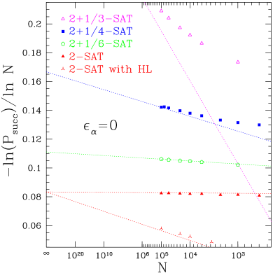
Figure 7: Comparison of eqs. (94)–(97) (lines) with empirical estimates (symbols) for the probability of success of the greedy UC algorithm on instances of the random $2+p$-SAT problem at the critical initial constraint-per-variable ratio $\alpha_{\mathrm{R}}(p)$ (i.e. $\epsilon_{\alpha}=0$) for p=0, $p=1/7$, $p=1/4$ and $p=1/3$, and data for the probability of success of the greedy HL algorithm kaporis-kirousis-lalas-hl-cl on instances of critical 2-SAT. The error bars are smaller than the symbols’ sizes. Data for $-\ln P_{\mathrm{success}}/\ln N$ are plotted against $1/\ln N$, and the straight lines come from our asymptotic analytical results, eqs. (94–97) (ignoring the $\mathcal{O}(N^{-1/3})$ terms), except for HL where it is a tentative extrapolation to $N=+\infty$.

5.2.4 The critical distribution of $C_{1}$

In the critical time regime ($T$ of the order of $N^{2/3}$), the PDF of $c=C_{1}/N^{1/3}>0$ is the solution $\rho$ of eq. (• ‣ 4.3). As a special case, the probability that no 1-clause is present is $\sigma\sim N^{-1/3}\rho(0)/2$. Convergence to this distribution, for $c>0$ on one hand and for $c=0$ on the other hand, is observed numerically — see Figure 8. The convergence is not uniform in the neighbourhood of $c=0$, which is expected since the distribution $\rho$ is singular in $c=0$. There is rather a cross-over from the regime where $C_{1}\ll N^{1/3}$ to the regime where $C_{1}$ is of the order of $N^{1/3}$. Eq. (39) yields, going to the $d_{2}\to 1$ limit (well-defined if $X_{1}>0$),

$$\pi_{0}(X_{1})=\sum_{C_{1}}P(C_{1})X_{1}^{C_{1}}=\frac{1-X_{1}}{1-X_{1}\exp(1-X_{1})}\pi_{0}(0)\ .$$ (98)

Hence (for large $N$ with fixed $X_{1}$)

$$G_{1}(X_{1})=N^{-1/3}\frac{\rho(0)}{2}\frac{1-X_{1}}{1-X_{1}e^{1-X_{1}}}+o\left(N^{-1/3}\right)\ .$$ (99)

The probabilities that $C_{1}$ takes the values 0, 1, 2, … are given by the coefficients of the Taylor expansion, in $X_{1}=0$, of $G_{1}$ above. It is observed that these probabilities converge very quickly to $N^{-1/3}\rho(0)$, which coincides with the $c\to 0$ limit of the distribution $\rho$ of $c=C_{1}/N^{1/3}$. These probabilities are plotted in the lower-left inset of Figure 8, together with numerical data for finite sizes. A good agreement is found.

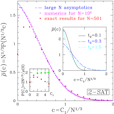
Figure 8: The normalized PDF $\overline{\rho}$ of $c=C_{1}/N^{1/3}$ for 2-SAT at the critical initial clauses-per-variable ratio $\alpha=1$ ($\epsilon_{\alpha}=0$) and at $t_{2}=0.3$. Long-dashed line: limit result for $\overline{\rho}$ at $N=+\infty$. Dots: numerical results from $8.10^{5}$ runs of the UC algorithm for $N=10^{5}$ ($\triangle$; the error bars are smaller than the symbol’s size) and results from the direct solution of eq. (34) for $N=501$ ($\blacksquare$) — see appendix E. Lower-left inset: probability $P$ (expressed in $N^{-1/3}\rho(0)/2$ units) that $C_{1}$ takes finite values at the $N=+\infty$ limit ($\bullet$). This shows how the discontinuity, at the scale of $c$, between $N^{1/3}P(C_{1}=0)=\sigma$ and $\lim_{c\to 0+}\overline{\rho}(c)=2\sigma$ is resolved at the scale of $C_{1}$. Numerical data (same as for the main plot) converge to $P$ when $N\to+\infty$. Upper-right inset: Normalized distributions $\overline{\rho}$ for $N=+\infty$ at times $t_{2}=0.1$ (solid line), $t_{2}=0.3$ (long dashes) and $t_{2}=1.5$ (short dashes).

5.2.5 Universality

For a given $p<2/5$, all algorithms that use the UP rule fall into the same universality class (which depends on $p$). They share the result eq. (92) with common $H$ (but $F(1)$ is a non-universal correction), and the critical distribution of $C_{1}$ studied in Section 5.2.4.

The reason is two-fold: first, the analysis done so far in Section 5 is still valid for another heuristic than R, run on random instances of the $2+p$-SAT problem, provided the critical trajectory starts on the $d_{2}=1$ line and is secant to it with some slope $\beta>0$. Second, the value of $\beta$ at criticality is universal and depends on $p$ only, because, at criticality, the heuristic is almost never used and UP alone fixes the slope: even if the resolution trajectories of several heuristics may be quite different in general (compare e.g. Eqs. (29) for R and (3.3) for GUC), in the critical regime, the probability that $C_{1}=0$ and the heuristic is used is of the order of $N^{-1/3}$ only. Most of the time, the UP rule is used, and the resulting evolution of $c_{2}$ and $c_{3}$ is common to all algorithms: the slope of the critical trajectory is $\beta(p)=(2-5p)/[2(1-p)]$ as for UC. We verified this by direct computation from eq. (29) for R, eq. (3.3) for GUC and the corresponding equations of reference kaporis-kirousis-lalas-hl-cl for HL and CL.

Figure 7 shows the agreement of empirical data for the HL heuristic, used on random 2-SAT instances, with the scaling of $P_{\mathrm{success}}$ that we derived for the R heuristic.

6 The 3-SAT class (stretched exponential class)

6.1 Equations and results for 3-SAT and its class

We now address the case $p>2/5$. Here, the critical resolution trajectory starts below the $d_{2}=1$ line and gets tangent to it, at point $(p=2/5,\alpha=5/3)$ at a finite time, $t^{*}\in]0,1[$. From eq. (29), $d_{2}(t)$ is locally a parabola around $t^{*}$ : $1-d_{2}(t-t^{*})\propto(t-t^{*})^{2}$. The critical resolution trajectory is at distance $\Delta=N^{-1/3}$ of the $d_{2}=1$ line as long as $t-t^{*}$ is of order $\Delta^{1/2}$: the exponent $a$ equals 1/2 here and the relevant equation is eq. (69), not eq. (• ‣ 4.3) as for 2-SAT. The computation is easier here (at least for the leading order) since we have an ordinary differential equation (the time enters into play only as a parameter of the coefficients of this ODE) rather than a partial derivatives equation. The relevant scaling for time is

$$T=t^{*}N+t_{3}N^{5/6}$$ (100)

according to eq. (60) where we replaced the notation $t_{0}$ with $t_{3}$ to emphasize that this scaling is proper to the 3-SAT class.

As for 2-SAT, the critical regime extends to a non-empty range of values of $\alpha$. This critical window is the same: we set

$$\alpha=\alpha_{\mathrm{R}}(p)(1+\epsilon_{\alpha}N^{-1/3})$$ (101)

with finite $\epsilon_{\alpha}$. Indeed, if $\alpha$ is less than $\alpha_{\mathrm{R}}(p)$ by more than $\Delta=N^{-1/3}$, because $d_{2}(t)$ is increasing proportionally with $\alpha$ (see Eqs. (28) and (29)), the resolution trajectory will be out of the critical region in particular at the time $t^{*}$ where $d_{2}(t)$ is maximal since $1-d_{2}(t)\gg\Delta$, and therefore at all times. Conversely, if $\alpha$ is above $\alpha_{\mathrm{R}}(p)$ by a distance much greater than $\Delta$, at time $t^{*}$ $1-d_{2}$ is an order of magnitude higher than the critical distance $\Delta$, which implies that the resolution trajectory would stay for an infinite duration, on the scale of $t_{3}$ in eq. (60) with $a=1/2$, above the $d_{2}=1$ line – this would yield numerous contradictions (0-clauses) and let the probability of success be exponentially small.

6.1.1 Results for the critical time regime

We now have to solve eq. (69). As for the 2-SAT family, we prefer to do computations on the (here normalized, or conditioned to success of the greedy algorithm) PDF $\overline{\rho}$ of the stochastic variable $C_{1}/N^{1/3}$ rather than on its generating function $\overline{\pi}$. Performing an inverse Laplace transform on eq. (69) yields

$$0=\frac{1}{2}\partial_{c}^{2}\overline{\rho}(c,t_{3})+e_{2}(t_{3})\partial_{c}\overline{\rho}(c,t_{2})+\frac{1}{2(1-t^{*})}[\overline{c}(t_{3})-c]\overline{\rho}(c,t_{3})$$ (102)

with the boundary condition

$$\frac{1}{2}\partial_{c}\overline{\rho}(0,t_{2})+e_{2}(t_{3})\overline{\rho}(0,t_{2})=0.$$ (103)

The parameters in eqs. (102) and (103) are $t^{*}=5/6-1/(3p)$ and $e_{2}(t_{3})=36t_{3}^{2}p^{2}/(p+2)^{2}-\epsilon_{\alpha}$.

Here, the initial condition is mostly irrelevant: the initial step of the algorithm, $T=0$ or $t^{*}\to-\infty$, is far out of the critical time region (finite $t^{*}$). When the resolution trajectory enters this region, the distribution of $C_{1}$ has already equilibrated to its critical value and is only subject to ‘adiabatic’ changes during the crossing of the critical region (Eq. (102) has no time derivative). Solving the ODE (102) brings out the explicit critical distribution of 1-clauses.

Let $u(c,t_{3}):=\overline{\rho}(c,t_{3})\exp[e_{2}(t_{3})c]$, $k(p)=[6p/(2+p)]^{-1/3}$ and

$$z:=\left[c-\overline{c}(t_{3})+\frac{2+p}{6p}e_{2}(t_{3})^{2}\right]/k(p)\ .$$ (104)

Eq. (102) is recast into an equation that admits Airy’s $\mathrm{Ai}$ and $\mathrm{Bi}$ functions as linearly independent solutions:

$$\partial_{z}^{2}u(z,t_{3})-zu(z,t_{3})=0.$$ (105)

See references in albright-airy for studies of eq. (105) in the context of (semi-classical) quantum mechanics or groeneboom-airy in the context of Brownian motion (similar to our situation). Since $u$ has to vanish for large $z$ (because $\overline{\rho}(c,t_{3})\to 0$ for large $c$) whereas $\mathrm{Bi}(z)$ is not bounded for large $z$, $u(z,t_{3})=A(t_{3})\mathrm{Ai}(z)$ where $A$ is a normalization coefficient. The boundary condition eq. (103) reads

$$\mathrm{Ai}^{\prime}(z_{0})/\mathrm{Ai}(z_{0})=-k(p)e_{2}(t_{3})$$ (106)

where $z_{0}$ is expressed from eq. (104) with $c=0$. Let $\mathcal{A}$ be the reciprocal function of $\mathrm{Ai}^{\prime}/\mathrm{Ai}$. Inverting eq. (106) yields an expression for $\overline{c}(t_{3})$:

$$\overline{c}(t_{3})=k(p)^{3}e_{2}(t_{3})^{2}-k(p)\mathcal{A}\left[-k(p)e_{2}(t_{3})\right]$$ (107)

and

$$\overline{\rho}(c,t_{3})=A(t_{3})e^{-e_{2}(t_{3})c}\mathrm{Ai}\left\{k(p)c+\mathcal{A}\left[-k(p)e_{2}(t_{3})\right]\right\}\ .$$ (108)

We did not compute explicitly the normalization constant $A(t_{3})$. The critical distribution $\overline{\rho}$ is plotted in Figure 9 for 3-SAT ($p=1$) and several values of $e_{2}$, to show the influence of the drift on its shape. The agreement with numerics is good; the same phenomenon in $c=0$ as for the 2-SAT family is observed: at $N=\infty$, $\overline{\rho}$ is singular, and for finite $N$ there is a cross-over from the regime $C_{1}\ll N^{1/3}$ to the regime $C_{1}=cN^{1/3}$ (see Sect. 5.2.4).

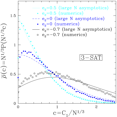
Figure 9: Critical distributions $\overline{\rho}$ for $c=C_{1}/N^{1/3}$ in the case of 3-SAT with drifts $e_{2}=0.5$ (solid line, $\bigcirc$), $e_{2}=0$ (dashed line, $\blacksquare$) and $e_{2}=-0.7$ (dotted line, $\triangle$). Points are from numerical estimates with size $N=10^{4}$.

The probability that the greedy algorithm doesn’t find a contradiction in the critical regime from time $t_{3}^{(1)}$ up to time $t_{3}^{(2)}$ satisfies, according to eq. (64) and the discussion preceding it,

$$-\ln p_{\mathrm{no-contr}}\left(t_{3}^{(1)}\to t_{3}^{(2)}\right)=$$

$$\qquad N^{1/6}\left[\mu\left(t_{3}^{(2)}\right)-\mu\left(t_{3}^{(1)}\right)\right]+\mathcal{O}\left(N^{-1/6}\right)\qquad$$ (109)

where, from eq. (65) and the initial condition $p_{\mathrm{no-contr}}(T=0)=1$, $\partial_{t_{3}}\mu=k(p)^{-3}\overline{c}(t_{3})/2$ and $\mu(t_{3})\to 0$ as $t_{3}\to-\infty$. In the interesting situation where $t_{3}^{(1)}<0<t_{3}^{(2)}$, using the $y$ variable such that $\mathrm{Ai}^{\prime}(y)/\mathrm{Ai}(y):=-k(p)e_{2}(t_{3})$ rather than $t_{3}$,

$$\mu\left(t_{3}^{(2)}\right)-\mu\left(t_{3}^{(1)}\right)=\frac{k(p)^{1/2}}{4}\times$$

$$\qquad\left(\int_{\mathcal{A}[k(p)\epsilon_{\alpha}]}^{\mathcal{A}[-k(p)e_{2}(-t_{3}^{(1)})]}+\int_{\mathcal{A}[k(p)\epsilon_{\alpha}]}^{\mathcal{A}[-k(p)e_{2}(t_{3}^{(2)})]}\right)\times$$

$$\qquad\frac{\mathrm{d}y}{\sqrt{k(p)\epsilon_{\alpha}-\mathrm{Ai}^{\prime}(y)/\mathrm{Ai}(y)}}\left[\frac{\mathrm{Ai}^{\prime}(y)^{2}}{\mathrm{Ai}(y)^{2}}-y\right]^{2}.\quad$$ (110)

Define (the integral is finite)

$$\Phi(x):=\frac{1}{4}\int_{\mathcal{A}(x)}^{+\infty}\frac{\mathrm{d}y}{\sqrt{x-\mathrm{Ai}^{\prime}(y)/\mathrm{Ai}(y)}}\left[\frac{\mathrm{Ai}^{\prime}(y)^{2}}{\mathrm{Ai}(y)^{2}}-y\right]^{2}\ .$$ (111)

For large positive $t_{3}^{(2)}$ (and similarly for large negative $t_{3}^{(1)}$),

$$\mu\left(t_{3}^{(2)}\right)-\mu(0)=\sqrt{k(p)}\Phi[k(p)\epsilon_{\alpha}]-\frac{k(p)^{3}}{4t_{3}^{(2)}}+\mathcal{O}\left({t_{3}^{(2)}}^{-5}\right)$$ (112)

where we have used a large-$t_{3}$ expansion of eq. (107). From eq. (100), $t_{3}$ is of order $N^{1/6}$ at most, thus eq. (112) allows one to express $\mu$ in terms of $\Phi$ only, up to corrections of the order of $N^{-1/6}$. Anticipating that the non-critical time regime, like the success case in Section 4.1, brings contributions to $\ln P_{\mathrm{success}}$ of order $\mathcal{O}(1)$ in $N$, the total probability of success (at time $T=N$) of the greedy UC algorithm reads

$$-\ln P_{\mathrm{success}}[(1+\epsilon_{\alpha})\alpha_{\mathrm{R}}(p),p]=$$

$$\qquad\qquad N^{1/6}2\sqrt{k(p)}\Phi[k(p)\epsilon_{\alpha}]+\mathcal{O}(1)\qquad$$ (113)

where the function $\Phi$ is closely related  to the universal function introduced in reference deroulers-monasson-universalite-up-lettre . It may easily be computed with a mathematical software and is plotted in Figure 10.

Let us heuristically check that the success and failure cases are recovered from the critical results when $\epsilon_{\alpha}$ tends to $-\infty$ and $+\infty$ respectively. Using the asymptotic expansions of $\mathrm{Ai}$ and $\mathrm{Ai}^{\prime}$ abramowitz+stegun ; sommabilite-developpement-asymptotique-airy , the asymptotic behaviour of $\Phi$ is found:

$$\Phi(x)\sim\frac{\pi}{8\sqrt{-x}} \text{when }x\to-\infty$$

$$\Phi(x)=\frac{4}{15}x^{5/2}-a\frac{\sqrt{x}}{2}+o(\sqrt{x}) \text{when }x\to+\infty$$

where $a\approx-2.338107410$ is the greatest zero of $\mathrm{Ai}$ on the real axis. Taking now $\epsilon_{\alpha}=N^{1/3}\epsilon$ shows that $-\ln P_{\mathrm{success}}\approx\pi/(4\sqrt{-\epsilon})$ for $\epsilon<0$, in agreement with eq. (49), and $-\ln P_{\mathrm{success}}\approx 4\epsilon N/15$, in agreement with the expected failure behaviour.

6.1.2 Matching critical and non-critical time scales — final result for $P_{\mathrm{success}}$

Here we use a heuristic reasoning, based on what we learned from the study of the 2-SAT family. On the one hand, the results from the previous paragraph show that the probability no to find a contradiction between times $t^{*}N$ and $T=t^{*}N+t_{3}N^{5/6}$ equals (with an obvious convention for negative $t_{3}$)

$$-\ln p_{\mathrm{no-contr}}(T=t^{*}N\to t^{*}N+t_{3}N^{5/6})=$$

$$\qquad N^{1/6}\left[\mu(t_{3})-\mu(0)\right]+R(t_{3},N)$$ (114)

where the function $R(t_{3},N)$ (assumed to be regular) is bounded when $N\to+\infty$ with fixed $t_{3}$. Setting $t_{3}=$ $(t-t^{*})N^{1/6}$ and using eq. (112),

$$-\ln p_{\mathrm{no-contr}}(T=t^{*}N\to tN)=N^{1/6}\sqrt{k(p)}\Phi[k(p)\epsilon_{\alpha}]\ \$$

$$\,-\frac{k(p)^{3}}{4}\frac{1}{t-t^{*}}+\mathcal{O}\left(N^{-1/6}\right)+R[(t-t^{*})N^{1/6},N].$$ (115)

On the other hand, out of the critical time regime, we may modify eq. (5.2.3) (with the expression of $d_{2}(t)$ for $\alpha=5/3$) to compute the lost of success probability in the large $N$ limit between given times on the scale of $T/N$. For $t<t^{*}$ and $t>t^{*}$ respectively,

$$-\ln p_{\mathrm{no-contr}}(T=0\to tN)=-\frac{k(p)^{3}}{4}\left(\frac{1}{t-t^{*}}+\frac{1}{t^{*}}\right)+$$

$$\qquad\frac{1}{4}\ln\left(\frac{t^{*}-t}{t^{*}}\right)+\int_{0}^{t}d\tau f(\tau)+\mathcal{O}\left(N^{-1/3}\right)$$ (116)

$$-\ln p_{\mathrm{no-contr}}(T=tN\to N)=$$

$$\qquad-\frac{k(p)^{3}}{4}\left(\frac{1}{1-t^{*}}-\frac{1}{t-t^{*}}\right)+$$

$$\qquad\frac{1}{4}\ln\left(\frac{1-t^{*}}{t-t^{*}}\right)+\int_{t}^{1}d\tau f(\tau)+\mathcal{O}\left(N^{-1/3}\right)$$ (117)

where $f$ is the function

$$f(t):=-\frac{3p}{2(p+2)}-\frac{9p^{2}}{(p+2)^{2}}(t-t^{*})\ .$$ (118)

Eqs. (6.1.2 – 6.1.2) share with eq. (6.1.2) a divergence in $1/(t-t^{*})$, but they also have a logarithmic divergence that does not appear in eq. (6.1.2). We speculate that, if we pushed the asymptotic expansion for large $N$ that led to eq. (6.1.2) one step further, we would find

$$R(t_{3},N)=g(t_{3})+S(t_{3},N)$$ (119)

with $g(t_{3})\sim\ln(|t_{3}|)/4$ when $t_{3}\to\pm\infty$ and with $S(t_{3},N)$ regular and bounded in the two limits, first $N\to+\infty$ with fixed $t_{3}$, then $t_{3}\to\pm\infty$. At this new order, the time-derivative term $\partial_{t_{0}}\overline{\pi}(x_{1},t_{0})$ that was canceled to write eq. (69) becomes relevant. It yields a correction to the probability of success that originates physically from the slow, ‘secular’, evolution of the shape of the probability distribution $\overline{\rho}$ of $c=C_{1}/N^{1/3}$: the solution of eq. (69) is the distribution of $c$ in a true stationary state, but here we have only a quasi-stationary situation ($c$ is slowly driven) and the actual distribution is always delayed w.r.t. the perfectly equilibrated solution of eq. (69).

With the assumption (119), eq. (6.1.2) reads, for $t\gtrless t^{*}$,

$$-\ln p_{\mathrm{no-contr}}(T=t^{*}N\to tN)=$$

$$\qquad N^{1/6}\sqrt{k(p)}\Phi[k(p)\epsilon_{\alpha}]\pm\frac{1}{24}\ln N\mp\frac{k(p)^{3}}{4}\frac{1}{t-t^{*}}$$

$$\qquad\pm\frac{1}{4}\ln|t-t^{*}|\mp g(0)+\mathcal{O}\left(N^{-1/6}\right)+$$

$$\qquad S[(t-t^{*})N^{1/6},N]$$ (120)

and comparing eq. (6.1.2) with eqs. (6.1.2 – 6.1.2) yields

$$S[(t-t^{*})N^{1/6},N]=\left\{\begin{array}[]{ll}F_{<}(t)+\mathcal{O}\left(N^{-1/6}\right)&\text{if }t<t^{*}\\ F_{>}(t)+\mathcal{O}\left(N^{-1/6}\right)&\text{if }t>t^{*}\\ \end{array}\right.$$ (121)

where $F_{<}$ and $F_{>}$ are two primitives of $f$. Replacing expressions (119) and (121) with $t=t^{*}+t_{3}N^{-1/6}$ in eq. (6.1.2) and using the regularity of $S$ in $t_{3}=0$ shows that

$$F_{<}(t)=F_{>}(t)=\int_{t^{*}}^{t}f(\tau)\mathrm{d}\tau\ .$$ (122)

Finally, adding eq. (6.1.2) for the two cases $t\gtrless t^{*}$ after making the substitution eq. (122) yields the total probability of success of the greedy algorithm UC=UP+R for $p>2/5$:

$$-\ln P_{\mathrm{success}}=N^{1/6}2\sqrt{k(p)}\Phi[k(p)\epsilon_{\alpha}]+E(p)+\mathcal{O}\left(N^{-1/6}\right)$$ (123)

with

$$E(p)=\frac{3p(p-4)}{2(p+2)^{2}}-\frac{3p}{2(5p-2)}+\frac{1}{4}\ln\left(\frac{6p}{5p-2}-1\right).$$ (124)

While the $N^{1/6}$ divergences of the two cases of eq. (6.1.2) add up, the $\ln N$ divergences cancel out. Similarly, if we set $t=t^{*}-\tau$ in eq. (6.1.2) and $t=t^{*}+\tau$ in eq. (6.1.2), add the results and let $\tau\to 0$, the $\ln|t-t^{*}|$ divergences cancel out. This seems reasonable since the slow adaptation of the shape of $\overline{\rho}$ is symmetric w.r.t. the time $t^{*}$: before $t^{*}$, the driving term in eq. (69) pushes $c$ away from 0 and the equilibration delay of the distribution of $c$ makes the actual $c$ smaller than the perfectly equilibrated $c$. Hence the $\ln N$ term in eq. (6.1.2) for $t<t^{*}$ has a negative contribution to the probability of finding two contradictory 1-clauses. Conversely, after $t^{*}$, the driving pulls $c$ towards 0 back. The delay of $c$ makes it larger than what the perfectly equilibrated $c$ would be. This yields a positive $\ln N$ correction in eq. (6.1.2). The balance of the two slow adaptations is null for symmetry reasons.

The corrections due to the fluctuations of $C_{2}$, temporarily left aside, have order, after eq. (3.3),

$$\mathcal{O}[N^{\delta-4/3}\exp(-N^{1/6}\Phi)]\text{ and }\mathcal{O}\left[N^{3/2-\delta}\exp\left(-N^{2\delta-1}/2\right)\right]$$

with possibles choices of $\delta$ in the range $]1/2,2/3[$. Taking $\delta$ in the range $]7/12,2/3[$ ensures that both corrections are negligible w.r.t. all terms of eq. (123).

The result (123) is compared to empirical success probabilities of the greedy UC=R+UP algorithm on a large number (2000 to $7\times 10^{5}$) of instances of the random 3-SAT problem with sizes up to $N=20000$ in Figure 10. In spite of strong finite-size effects (in $1/N^{1/6}$), there is an excellent agreement because eq. (123) provides also the first subdominant term.

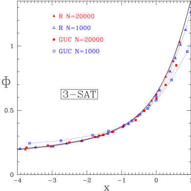
Figure 10: Empirical data for the probability of success of the greedy algorithms with R and UC heuristics on $10^{3}$ to $7\times 10^{5}$ instances of the random 3-SAT problem, for several initial clauses-per-variable ratios. Error bars are smaller than the symbol’s sizes. Dotted lines are guides for the eye. Data are plotted after rescaling their $x$ and $y$ axis with coefficients $r^{\Phi}$ and $r^{\epsilon}_{\alpha}$ to compare them with universal scaling function $\Phi$ (solid line), according to eq. (6.1.3).

6.1.3 Universality

Any heuristic H run on a set of random instances with self-averaging $C_{2}$ and a typical $C_{2}$ such that, for a given initial constraint-per-variable ratio $\alpha$, the resolution trajectory becomes tangent to the $d_{2}=1$ line at a finite time $t^{*}\in]0,1[$ with

$$1-d_{2}(t-t^{*})\propto(t-t^{*})^{2}$$ (125)

has the same critical behaviour as $R$. Indeed, in such a case, the generating function for $C_{1}$ satisfies eq. (34) and one may use critical scalings for the quantities $C_{1}$, $T$, $\alpha$ and $P_{\mathrm{success}}$ to derive eq. (102) from eq. (34). In these scalings, the exponents are independent of H because the geometric situation expressed by eq. (125) is the same as for heuristic R. Solving eq. (102) yields the same scaling function $\Phi$ as for the R heuristic, i.e. there exists numbers $\alpha_{H}$, $r_{H}^{\Phi}$ and $r_{H}^{\epsilon_{\alpha}}$ (that depend on H and p) such that 

$$-\ln P_{\mathrm{success}}[\alpha_{H}(1+\epsilon_{\alpha}N^{-1/3})]=$$

$$\qquad N^{1/6}\;r_{H}^{\Phi}\ \Phi\left(r_{H}^{\epsilon_{\alpha}}\;\epsilon_{\alpha}\right)+E_{H}+\mathcal{O}\left(N^{-1/6}\right).\quad$$ (126)

$E_{H}$ is a non-universal correction (even the contribution from a primitive of the universal term $\ln|t-t^{*}|/4$ in eq. (6.1.2) to $E_{H}$ is not universal because $t^{*}$ depends on H). Scaling relation (6.1.3) is expected to hold for most, if not all, algorithms using UP on random $2+p$-SAT instances with $p>2/5$. For GUC we performed analytic computations on the basis of eq. (3.3). The values of the numbers above are, in the case of $p=1$, i.e. random 3-SAT, with GUC heuristic:

$$\alpha_{\mathrm{GUC}}\approx 3.003494331$$

$$\qquad\text{ is such that }3\alpha_{\mathrm{GUC}}/2-\ln(3\alpha_{\mathrm{GUC}}/2)=3$$

$$r_{\mathrm{GUC}}^{\Phi}=\alpha_{\mathrm{GUC}}^{-1/12}\alpha_{\mathrm{R}}(1)^{1/12}2^{5/6}\approx 1.764223038$$

$$r_{\mathrm{GUC}}^{\epsilon_{\alpha}}=(3\alpha_{\mathrm{GUC}}/4-1/2)\alpha_{\mathrm{GUC}}^{-1/6}\alpha_{\mathrm{R}}(1)^{1/6}2^{-1/3}$$

$$\qquad\ \,\approx 1.363750542$$

$$F_{\mathrm{GUC}}(1)\approx-1.2438849.$$

Empirical data for the probability of success of the UP+ GUC algorithm are compared with the universal function $\Phi$ in Figure 10 — as for heuristic R, the agreement is very good, despite strong finite-size effects.

Notice also that the point where the critical resolution trajectory gets tangent to the $d_{2}=1$ line is universal. At this point, the residual 2-clauses-per-unassigned-variables ratio $d_{2}=\alpha(1-p)=1$ and the residual 3-clauses-per-unassigned-variables ratio $\alpha p=3/2$ so that each affectation of variable through UP produces, in average, a new 2-clause from the remaining 3-clauses — this is why $d_{2}(t)$ has a vanishing derivative and the trajectory does not cross the $d_{2}=1$ line. Moreover, the resolution trajectory (e.g. its curvature) is locally the same for all heuristics since almost all time steps use UP; the chances that the heuristic rule is used in one step during the critical regime scale like $P(C_{1}=0)\sim N^{-1/3}$. Therefore, improving some heuristic may only affect the pre- and post-critical time regimes. A good heuristic is one that does its best to avoid the critical region, or to delay entering it as much as possible.

6.2 The special case of 2+2/5-SAT

6.2.1 The tricritical point $(p=2/5,\alpha=5/3)$

For $p=2/5$, the critical window for $\alpha$ is the same as for 2- and 3-SAT, $\alpha=5/3(1+\epsilon_{\alpha}N^{-1/3})$. The critical resolution trajectory is tangent to the $d_{2}=1$ line so that $-\ln P_{\mathrm{success}}$ scales like $N^{1/6}$ like in the 3-SAT class. In addition, the delay of the actual distribution $\overline{\rho}$ of $c=C_{1}/N^{1/3}$ w.r.t. the fully equilibrated distribution that solves eq. (69) contributes to the success probability with a non-vanishing subdominant $\ln N$ term. This is because, instead of reversing its direction, the driving of $c$ is directed towards 0 during the whole algorithm’s run, for the critical resolution trajectory starts on the $d_{2}=1$ line.

For times $T$ of the order of $N^{5/6}$, eq. (102) is relevant (with $t^{*}=0$ and $e_{2}(t_{3})=t_{3}^{2}-\epsilon_{\alpha}$). In the expression (6.1.1), $k(p)=1$ and $t_{3}^{(1)}$ has to be 0. This yields

$$-\ln P_{\mathrm{success}}\left[\frac{5}{3}(1+\epsilon_{\alpha}),\frac{2}{5}\right]=\Phi(\epsilon_{\alpha})N^{1/6}+o(N^{1/6}).$$ (127)

The critical distribution $\overline{\rho}$ of $C_{1}/N^{1/3}$ is the same as for the 3-SAT family, up to scaling factors.

As for 3-SAT, we did not compute directly the correction due to secular evolution of $\overline{\rho}$ , but we deduced its contribution to the final result by comparison between the time scales of $t_{3}=T/N^{5/6}$ and of $t=T/N$. For fixed $t$ and large $N$, eq. (6.1.2) reads here

$$-\ln p_{\mathrm{no-contr}}(T=0\to tN)=N^{1/6}\Phi(\epsilon_{\alpha})+\frac{1}{24}\ln N-\frac{1}{4\,t}$$

$$\qquad+\frac{1}{4}\ln t-g(0)+\mathcal{O}\left(N^{-1/6}\right)+S(tN^{1/6},N)$$ (128)

while eq. (6.1.2) reads

$$-\ln p_{\mathrm{no-contr}}(T=tN\to N)=\frac{1}{4}\left(\frac{1}{t}-1\right)-\frac{1}{4}\ln t$$

$$\qquad-\frac{3}{8}+\frac{1}{4}t+\frac{1}{8}t^{2}+\mathcal{O}\left(N^{-1/3}\right).$$ (129)

Thus $S(tN^{1/6},N)=-t/4-t^{2}/8+g(0)$, and

$$-\ln P_{\mathrm{success}}=N^{1/6}\Phi(\epsilon_{\alpha})+\ln(N)/24-5/8+o(1)\ .$$ (130)

This expression compares well with numerical estimates in the critical $\epsilon_{\alpha}=0$ case, see Figure 11.

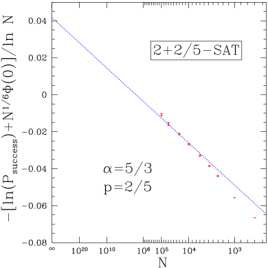
Figure 11: Comparison of empirical estimates of $P_{\mathrm{success}}$ with prediction eq. (130) for $\epsilon_{\alpha}=0$. We plot $-[\ln P_{\mathrm{success}}+\Phi(0)]/\ln(N)$ as a function of $1/\ln(N)$. The straight line is the analytical prediction, $1/24-5/8/\ln(N)$.

As a side remark, in the range of time steps of the order of $N^{2/3}$, eq. (77) with vanishing $\beta(p)$ is relevant. Numerical evidence shows that its solution $\rho$, once normalized, converges to the PDF $\overline{\rho}$ that satisfies eq. (102) with $e_{2}=t^{*}=0$, which is natural since $\overline{\rho}$ is the stationary solution of eq. (77). This equilibration process takes a finite range of time $T/N^{2/3}$, but a vanishing range of time $t_{3}$: this is why the solution of eq. (102) yields a finite value for $\overline{c}(t_{3}=0)$, whereas $C_{1}$ at $T=0$ is 0.

For $p=2/5$, the scaling function $\Phi$ is truly universal, in the sense that $r^{\epsilon_{\alpha}}=r^{\Phi}=1$ for all heuristics. Indeed, the resolution starts already in the critical regime where UP is used at almost every step and the heuristic becomes irrelevant; the trajectory $d_{2}(t)$ is then locally universal.

6.2.2 Matching the 2-SAT family with the 3-SAT class

The refined scaling $p=2/5(1+\epsilon_{p}N^{-1/6})$ allows us to blow up the transition between the 2-SAT family where $P_{\mathrm{success}}$ decays algebraically with exponent $\gamma(p)$ and the 3-SAT class where it decays as a stretched exponential. Now, the critical window for $\alpha$ is $\alpha=\frac{5}{3}(1+\frac{2}{3}\epsilon_{p}N^{-1/6}+\epsilon_{\alpha}N^{-1/3})$, $e_{2}(t_{3})=(t_{3}-\frac{5}{6}\epsilon_{p})^{2}-\frac{1}{4}\epsilon_{p}^{2}-\epsilon_{\alpha}$ and

$$-\ln P_{\mathrm{success}}=N^{1/6}\Phi(\epsilon_{\alpha},\epsilon_{p})+\ln(N)/24+\mathcal{O}(1)$$

with

$$\Phi(\epsilon_{\alpha},\epsilon_{p}) = \frac{1}{4}\int_{\mathcal{A}[\epsilon_{\alpha}-\frac{4}{9}\epsilon_{p}^{2}]}^{+\infty}\frac{\mathrm{d}y}{\sqrt{\epsilon_{\alpha}+\frac{1}{4}\epsilon_{p}^{2}-\mathrm{Ai}^{\prime}(y)/\mathrm{Ai}(y)}}\times$$ (131)

$$\qquad\qquad\left[\frac{\mathrm{Ai}^{\prime}(y)^{2}}{\mathrm{Ai}(y)^{2}}-y\right]^{2}$$

for $\epsilon_{\alpha}\leq\frac{4}{9}\epsilon_{p}^{2}$ and $\epsilon_{p}\leq 0$. If we send $\epsilon_{p}$ to $-\infty$ (as e.g. $-N^{1/6}q$) with $\epsilon_{\alpha}\ll\frac{4}{9}\epsilon_{p}^{2}$, $\Phi$ behaves like $1/\epsilon_{p}$ and $P_{\mathrm{success}}$ is finite. This was expected since, in this case, we dive into the success region below the $d_{2}=1$ line. However, if we follow the $d_{2}=1$ line and set $\epsilon_{\alpha}=\frac{4}{9}\epsilon_{p}^{2}$, $\Phi$ behaves like $-\ln(\epsilon_{p})/\epsilon_{p}$ and $-\ln P_{\mathrm{success}}=\ln(N)[1/24-1/(20q)]$ to the leading order in $N$, which matches the singularity (51).

6.3 Case of K-SAT with $K\geq 4$

For general $K$, that is for random instances with initially $N$ variables and $C_{2}$ 2-clauses, $C_{3}$ 3-clauses, …, $C_{K}$ $K$-clauses, $d_{2}(t)$ may become tangent to the $d_{2}=1$ line with an exponent greater than 2: $1-d_{2}(t-t^{*})\propto(t-t^{*})^{n}$ with $n<K$, and the scaling exponent $\lambda$ for $-\ln P_{\mathrm{success}}$ may take the value $\frac{1}{3}(1-\frac{1}{n})$. This happens when reduction of $j$-clauses into $j-1$-clauses compensates exactly the lost of $j-1$-clauses for $j\geq 4$, so that $d_{2}(t)$ stays longer close to the critical $d_{2}=1$ line. $n$ is necessarily integer because $c_{2}$ is computed after solving a triangular system of equations like (27). When $n$ is odd, the critical resolution trajectory crosses (with vanishing slope) the $d_{2}=1$ line, coming from the failure region ($d_{2}>1$) into the success one. Thus the critical behaviour may be reached only if the trajectory starts on this line (initial $C_{2}=N$; otherwise, the trajectory stays for a number of time steps $0\leq T\leq N$ of the order of $N$ in the failure region $d_{2}>1$ and the probability of success vanishes exponentially), and $-\ln P_{\mathrm{success}}$ is necessary accompanied with a $\ln N$ subleading term (because of the secular equilibration of the critical distribution of $C_{1}$, like in the $2+2/5$-SAT case).

The critical behaviour of the 2-SAT family is recovered if the initial clauses-per-variable ratios $\alpha_{j}=C_{j}/N$ are low enough, with initial $\alpha_{2}=1$, so that the resolution trajectory is secant to the $d_{2}=1$ line at time $t=0$. The results for the R heuristic are universal (see Sect. 5.2.5) and eq. (32) leads to

$$P_{\mathrm{success}}\propto N^{\frac{1}{12\left(1-\frac{3C_{3}}{2C_{2}}\right)}}$$ (132)

provided $\alpha_{2}=1$, $\alpha_{3}/\alpha_{2}<2/3$, $\alpha_{4}/\alpha_{3}<1$, $\alpha_{5}/\alpha_{4}<6/5$, $\ldots$, $\alpha_{K}/\alpha_{K-1}<2(K-2)/K$.

As for $2+p$-SAT, the critical initial clauses-per-variable ratios that yield a stretched-exponential behaviour are not universal, but the position where the resolution trajectory meets the $d_{2}=1$ hyperplane (with exponent $n$) in the space of the $\alpha_{j}$’s is. It lies on the boundary of the region that inequalities above define: if $n=2$, $\alpha_{2}=1$, $\alpha_{3}=2/3$ and $\alpha_{4}<2/3$. If $n=3$, $\alpha_{4}=2/3$ additionally but $\alpha_{5}<4/5$, and so on. The trajectory can’t reach tangentially the boundary twice (because, in the neighbourhood of the points where the boundary is hit tangentially, the flow is going away; coming for a second time to one of these points would need to re-increase some clauses-per-variable ratios, which is impossible precisely because of the inequalities above); thus $-\ln P_{\mathrm{success}}$ can have at most one power-law divergence (i.e. only one power of $N$) and one $\ln N$ divergence (always present when $n$ is odd).

In the situation where the greatest power of $N$ that appears in $-\ln P_{\mathrm{success}}$ is $(1-1/n)/3$, the technique of computation based on eq. (3.3) may still be applied, provided that $\delta\in]2/3-1/(6n),2/3[$. The shrinking of this interval as $n\to+\infty$ probably means that large deviations of $c_{2}$ for finite size $N$ have more and more influence (on the statistics of $C_{1}$ and on $P_{\mathrm{success}}$) as $n$ is increased.

7 Discussion and perspectives

7.1 How well does UP estimate the ground state energy of $2+p$-SAT formulas?

At the critical initial constraint-per-variable ratio $\alpha$, the probability $P_{\mathrm{success}}$ that an algorithm using the UP rule finds a satisfying assignment to a random formula vanishes algebraically with large $N$. In contrast, for 2-SAT and $\alpha=1$, such a satisfying assignment exists with finite probability bollobas-borgs-chayes-2sat-scaling-window , that we numerically estimated to $0.907\pm 10^{-3}$ – see Appendix A. To this respect, even though the dynamic threshold of algorithms using the UP rule is equal to the static threshold $\alpha_{C}(p)$ for $p<2/5$, they perform not very well at the threshold (at least for $p=0$). But we argue here that they don’t overestimate too much the minimum number of clauses that can be satisfied simultaneously in an instance of SAT. This number is also commonly referred to as the ground state energy of the instance. Finding it amounts to solve the so-called MAX-SAT optimization problem, and, like the SAT problem papadimitriou-steiglitz-livre , this problem is classified as difficult by the computer scientists. It is known to grow like $(\alpha-\alpha_{\mathrm{R}})^{3}$ for $\alpha>\alpha_{\mathrm{R}}$ monasson-zecchina-statistical-mechanics-of-random-K-sat .

If we allow the greedy algorithm to keep running even if 0-clauses are found, the final number $C_{0}$ of 0-clauses is an upper bound to the ground state energy. The average $C_{0}$ may be computed from the generating function $G_{01}$ that satisfies eq. (34) with $X_{0}=1$. Using non-zero values of $X_{0}$ doesn’t modify substantially the computations of $G_{1}$ that we did so far. Eq. (77) reads now

$$\partial_{t_{2}}\rho(c,t_{2})=\frac{1}{2}\partial_{c}^{2}\rho(c,t_{2})+\beta(p)t_{2}\partial_{c}\rho(c,t_{2})-\frac{1-X_{0}}{2}c\rho(c,t_{2})$$ (133)

and eq. (5.2.3) becomes

$$G_{01}(\to tN^{1/3};X_{0},X_{1}=1)=$$ (134)

$$\quad\frac{1-X_{0}}{12\beta(p)}\ln N+\frac{\ln t}{4\beta(p)}+H[X_{0},\epsilon_{\alpha},\beta(p)]+\mathcal{O}\left(\frac{1}{t^{3}N}\right)$$

where $H$ depends also on $X_{0}$. Deriving eq. (134) w.r.t. $X_{0}$ and setting $X_{0}=1$ yields

$$\langle C_{0}\rangle(\to tN^{1/3})=$$ (135)

$$\quad\frac{1}{12\beta(p)}\ln N+\partial_{X_{0}}H[X_{0},\epsilon_{\alpha},\beta(p)]\big{|}_{X_{0}=1}+\mathcal{O}\left(\frac{1}{t^{3}N}\right).$$

We know that, if $X_{0}=0$, $H[X_{0},\epsilon_{\alpha},\beta(p)]$ behaves like $\epsilon_{\alpha}^{3}$ for large positive $\epsilon_{\alpha}$. Assuming that the behaviour is the same for general $X_{0}$, the average number of 0-clauses at the end of the critical time regime is

$$\langle C_{0}\rangle(\to tN^{1/3})\approx h(p)[\alpha-\alpha_{\mathrm{R}}(p)]^{3}N+\frac{1}{12\beta(p)}\ln N+\mathcal{O}(1)$$ (136)

for some universal number $h(p)$ (as in Section 5.2.5, in the critical regime the heuristic is almost never used, only UP is used, hence $h(p)$ is universal, or, in other words, independent of the heuristic). The subsequent non-critical time regime $N^{1/3}\lesssim T\leq N$ brings only a finite contribution to $\langle C_{0}\rangle$. Therefore, algorithms using UP give an upper bound to the ground state energy of $2+p$-SAT problems with $p<2/5$ that grows with $\alpha$ like $h(p)(\alpha-\alpha_{\mathrm{R}})^{3}$. This speculation agrees well with numerical results for the average $C_{0}$ at the end of runs of UC=UP+R or UP+HL on instances of 2-SAT, see Figure 12. The scaling $\langle C_{0}\rangle\propto N^{1/12}$ is also numerically correct (not shown on the figure).

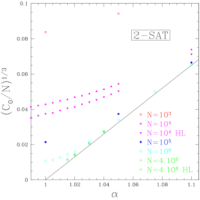
Figure 12: Numerical test of the scaling relationship (136) for the UC=UP+R and UP+HL algorithms on 2-SAT (data are for heuristic R when not otherwise stated). The rescaled average number of 0-clauses $(\langle C_{0}\rangle/N)^{1/3}$ is plotted vs. the initial clauses-per-variable ratio $\alpha$. The error bars are smaller than the symbol’s sizes. The solid line is a tentative fit with slope $0.65\approx 0.27^{1/3}$. For $\alpha=1$, finite-size effects are strong since $\langle C_{0}\rangle$ decreases with $N$ as $N^{-1/12}$, which is consistent with eq. (136). Using the HL heuristic rather than the fully random R heuristic gives some improvement for finite sizes, but no improvement in the thermodynamic limit because the heuristic plays no role in the critical regime.

The exponent 3 in $h(p)(\alpha-\alpha_{\mathrm{R}})^{3}$ agrees with the (non-rigorous) results for the ground state energy of random 2-SAT computed in Section VI of monasson-zecchina-statistical-mechanics-of-random-K-sat . However, the numerical estimate $h(0)\approx 0.27$ (see Fig. 12) is clearly different from the coefficient 0.15 computed in Section VI of monasson-zecchina-statistical-mechanics-of-random-K-sat : the bound that UP provides is not tight . As a side remark, general rigorous results hastad-inapproximabilite-max-2sat-conference ; hastad-inapproximabilite-max-2sat-journal show that, using techniques quite different from UP, one can design an algorithm running in polynomial time that finds, for any instance of random 2-SAT, an assignment which satisfies at least 93.1% of the number of clauses that can be satisfied simultaneously in that instance (let us call this number optimum of the instance; it is the difference between the number of clauses and the ground state energy). Conversely, it is proved impossible to find a polynomial time-algorithm that would, for each instance, satisfy simultaneously a number of clauses of at least $21/22\approx$ 95.5% of the optimum (for 3-SAT, these two bounds become $7/8$). For 2-SAT, our results state that, in average, the polynomial time greedy algorithms that use UP outperform these worst-case bounds for $\alpha$ close to $\alpha_{\mathrm{R}}$ (they satisfy in average a number of clauses that tends to the optimum as $\alpha$ tends to $\alpha_{\mathrm{R}}$, although on some rare instances they may perform badly). It might be interesting to know the average behaviour of the algorithms of hastad-inapproximabilite-max-2sat-conference ; hastad-inapproximabilite-max-2sat-journal and see whether they get closer to the ground state energy as algorithms based on UP.

7.2 Interpretation as a random graph percolation phenomenon

Introduction of the oriented graph $\mathcal{G}$ representing 1- and 2-clauses allows us to re-interpret some of the scalings that we found in the previous sections. $\mathcal{G}$ is made of $2\,(N-T)$ vertices (one for each variable $x_{i}$ and its negation $\bar{x}_{i}$), $C_{1}$ marked vertices (one for each 1-clause $z_{i}$), and $2\,C_{2}$ edges ($z_{i}\vee z_{j}$ is represented by two oriented edges $\bar{z}_{i}\to z_{j}$ and $\bar{z}_{j}\to z_{i}$) aspvall-plass-tarjan-temps-lineaire ; bollobas-borgs-chayes-2sat-scaling-window . $d_{2}$ is simply the average (ingoing or outgoing) degree of vertices in $\mathcal{G}$.

A step of UP removes a marked vertex, say $z$, and its attached outgoing edges, after having marked its descendants (2-clauses with $\bar{z}$ are reduced). If $\bar{z}$ appears in some 3-clauses, these clauses become 2-clauses, i.e. new pairs of edges in $\mathcal{G}$. UP-steps are repeated until no vertex is marked, then some vertex is marked according to the heuristic of the algorithm and another round of UP starts. During a round, there is a competition between the elimination of edges and vertices and the creation of new edges. All vertices in the (outgoing-edges) connected component of the initial $\mathcal{G}$ that started with the first marked vertex are removed. In addition, the vertices that have been linked to this component through the new edges are also removed. A contradiction arises (a 0-clause appears) when two conjugate vertices $z$ and $\bar{z}$ are marked. When $\mathcal{G}$ percolates (this happens for $d_{2}\geq 1$ janson-luczak-rucinski-livre ; bollobas-borgs-chayes-2sat-scaling-window ), there exist many oriented loops going from one literal $z$ to its conjugate and back to it aspvall-plass-tarjan-temps-lineaire . Marking a vertex of such a loop results sooner or later in the marking of both $z$ and $\bar{z}$, and the algorithm fails. Conversely, if $\mathcal{G}$ doesn’t percolate, there is no such loop with finite probability. The success/failure transition of the algorithms using UP is related to the percolation transition of $\mathcal{G}$; if the value of $d_{2}$ is bounded away from 1, $\mathcal{G}$ never percolates and the probability of success if finite. Although the results for percolation of random graphs were obtained in a static context, they apply readily to the graph $\mathcal{G}$ that is kinetically built, because of conditional uniformity (see Sect. 3.1).

Notice that the percolation phenomenon of random graphs is very robust. For instance, taking random graphs conditioned to a certain degree distribution of the vertices newman-strogatz-watts-gral-avec-distribution-degres does not change the universality class if the probability of the large degrees decays not too slowly. Such (directed) graphs $\mathcal{G}$ appear in the context of algorithms with the HL or CL heuristics that select literals according to their degrees. We have checked numerically for HL that the degree distribution in $\mathcal{G}$ is far from the Poisson distribution that we find for non-conditioned $\mathcal{G}$’s (e.g. for R and GUC). Still, the probabilities of finding vertices of high degrees decrease fast and $\mathcal{G}$ has the same percolation critical behaviour as a random graph. A parallel can be drawn between the robustness of the critical behaviour of random graphs and, in our computation, the weak dependence of the probability law for $C_{1}$ on that of $C_{2}$ (only the average of $C_{2}/N$ matters thanks to self-averaging).

In the percolation critical window $|d_{2}-1|\sim N^{-1/3}$ janson-luczak-rucinski-livre ; bollobas-borgs-chayes-2sat-scaling-window , the probability that a vertex belongs to a component of size $S$ is $Q(S)\sim S^{-3/2}$ newman-strogatz-watts-gral-avec-distribution-degres , with a cut-off equal to the largest size, $N^{2/3}$. From Figure 3, departure ratios $\alpha$ have to differ from $\alpha_{\mathrm{flat}}$ by $N^{1/3}$ for resolution trajectories to fall into the critical window. Hence the critical window in $\alpha$ has width $N^{-1/3}$ for both the 2-SAT family and the 3-SAT class.

When the resolution trajectory is tangent to the $d_{2}=1$ line (3-SAT class), it spends the time $\Delta t\sim\sqrt{|d_{2}-1|}\sim N^{-1/6}$ in the critical window, corresponding to $\Delta T=N\,\Delta t\sim N^{5/6}$ eliminated variables. Let $S_{1},S_{2},\ldots,S_{J}$ be the sizes of components eliminated by UP in the critical window; we have $J\sim\Delta T/(\int\!\mathrm{d}S\,Q(S)\,S)\sim N^{1/2}$. During the $j^{th}$ elimination, the number of marked vertices ‘freely’ diffuses, and reaches $C_{1}\sim\sqrt{S_{j}}$. The probability that no contradiction occurs is $[(1-q)^{C_{1}}]^{S_{j}}\sim\exp(-S_{j}^{3/2}/N)$ where $q\sim\frac{1}{N}$ is the probability that a marked vertex is the negation of the one eliminated by UP. Thus $-\ln P_{\mathrm{success}}\sim J\!\int\!\mathrm{d}S\,Q(S)\,S^{3/2}/N\sim N^{1/6}$, giving $\lambda=\frac{1}{6}$. Notice that, while the average component size is $S\sim N^{1/3}$ (and thus the probability that $C_{1}$ vanishes in the critical time regime is $\sim N^{-1/3}$, consistently with Eq. (56)), the value of $\lambda$ is due to the largest components with $S\sim N^{2/3}$ i.e. $C_{1}\sim N^{1/3}$ marked vertices.

In the case of the 2-SAT family, the algorithm eliminates only $\Delta T\sim N^{2/3}$ variables and $J\sim N^{1/3}$ connected components. The estimation above yields a finite $-\ln P_{\mathrm{success}}$ and fails to predict the correct answer because it doesn’t take the $\ln N$ corrections into account.

For general $K$-SAT, one may attach to an instance a family of oriented hypergraphs were vertices are the literals and the $l$-clauses are $l$-hyperedges, for $2\leq l\leq L$ and some fixed integer $L$ between 2 and $K$. The first graph of this family, for $L=2$, is $\mathcal{G}$. The critical behaviours exhibited in Section 6.3 appear when the first hypergraphs, $2\leq l\leq L$ for some $3\leq L\leq K$, percolate. This happens goldschmidt-percolation-hypergraphes for clauses-per-variable ratios $\alpha_{l}=2^{l-1}/[l(l-1)]$ for $2\leq l\leq L$; then $-\ln P_{\mathrm{success}}\sim N^{\lambda}$ with $\lambda=\frac{1}{3}(1-\frac{1}{L-1})$.

7.3 Unit-Propagation in other problems

The Unit-Propagation rule that we defined for SAT problems may easily be generalized to other contexts. In the graph coloring problem, one wants to know if the vertices of a given graph may be colored with $K$ colors in such a way that no two vertices that share an edge have the same color. A family of algorithms that deal with such graphs processes the graph by maintaining the list of available colors on each vertex (initially the list of all $K$ colors) achlioptas-molloy-coloriage-par-liste ; ein-dor-monasson-coloriage-symetrique . When a vertex is colored with some color, this color is removed from the list of available colors of the neighbours of this vertex. The UP rule would be defined as: “When, on the partially colored graph, at least one vertex has only one available color, color it with this color prior to any other action”. We expect eq. (34) to hold also for such graph coloring algorithms, after choosing a relevant value for $C_{2}$. This value may be computed by the technique of differential equations achlioptas-molloy-coloriage-par-liste ; ein-dor-monasson-coloriage-symetrique like in eqs. (27). The probability of success of the randomized, greedy coloring algorithms should behave like $P_{\mathrm{success}}$ for $K$-SAT; in particular, for the case of 3 colors, it should have a success-to-failure transition with critical behaviour in $N^{1/6}$.

Similarly, the study of greedy algorithms using UP for other hard decision computational problems garey-johnson-intractability should lead to the same critical behaviour (that is, problems where the answer of the algorithm should be either “yes – satisfiable – colorable – …” or “no – unsatisfiable – uncolorable – …”).

In the framework of error-correcting codes, the authors of reference amraoui-montanari-richardson-urbanke-taille-finie also found a critical behaviour that is governed by a Brownian motion with parabolic drift groeneboom-airy , which leads to Airy distributions, as we found for $C_{1}$ in Section 6.

There is another important family of problems, called optimization problems, where the answer is a number. For example, in the MAX-SAT problem, believed to be a hard computational problem, one wants to know, for some instance of SAT, the maximal number of satisfied clauses or, equivalently, the ground state energy, i.e. the minimal number of violated clauses over all assignments of variables of this instance. In the context of graph coloring, one may look for the minimal number of colors needed to color some graph, etc. Knowing whether their random formulation (where instances are drawn uniformly at random) fall into the same universality classes as the random SAT problem requires more investigation. However, each optimization problem has a decision version, which can be related to this work. For instance, the decision version of random MAX-$2+p$-SAT would be: “is there an assignment of the variables of this instance such that the number of violated clauses does not exceed some fixed number $m$?” We can deal with it by asking for the probability that the greedy algorithm using UP ends, after having assigned all variables, with a number $C_{0}$ of 0-clauses that does not exceed $m$. As long as $m$ is bounded in the large $N$ limit, this new success probability can be computed by summing the 0th, 1st, 2nd, …, $m$th derivatives of $G_{01}(X_{0},1;N|C_{2})$ with respect to $X_{0}$ in $X_{0}=0$. A dynamic phase transition between success and failure phases is found as for the random $2+p$-SAT problem and, both for $p<2/5$ and $p\geq 2/5$, the largest term in the expression for $-\ln P_{\mathrm{success}}$ at criticality is independent of $m$: the critical exponents are unchanged, although subdominant terms now depend on $m$ (in particular, for $p<2/5$, terms in $m\ln(\ln(N))$ appear in the expression of $-\ln P_{\mathrm{success}}$ at criticality). We expect the exponents to remain the same for algorithms using UP on the decision version of other optimization problems. It would be interesting to know what happens when $m$ is allowed to become large with $N$.

Another interesting question is whether instances of SAT (or other problems) with strong correlations, such that self-averaging of $C_{2}$ is lacking, would lead to new universality classes. This could be the case for instances of SAT such that $\mathcal{G}$ can be embedded into a finite-dimensional space, or with a power-law distribution of the number of occurrences of variables in clauses, possibly built by preferential attachment of new variables to highly-connected old variables. Graphs with such features are observed in real-world applications such as the ‘World Wide Web’ or social networks; they might be helpful in modeling industrial instances of SAT better than the random, ‘flat’ distribution.

Acknowledgments. We thank Andrea Montanari and Federico Ricci-Tersenghi (who motivated the study in Section 7.1) for stimulating discussions. Partial financial support from the‘Statistical physics of Information Processing and Combinatorial Optimization’ (STIPCO) Network of the Research Training Network programme of the European Commission and from the French Ministry of Research through the ‘ACI Jeunes Chercheurs’ ‘Algorithmes d’optimisation et systèmes désordonnés quantiques’ is acknowledged. We thank the Laboratoire de Physique Théorique in Strasbourg, where part of this work was realized, for its hospitality.

Appendix A Numerical estimate of the probability of satisfiability for critical 2-SAT

Reference bollobas-borgs-chayes-2sat-scaling-window rigorously proves that the probability of a random 2-SAT formula of size $N$ with initial constraint-per-variable $\alpha=1$ is finite (whereas it vanishes for large $N$ if $\alpha>1$). A numerical estimate of this probability was given on figure 5 of reference shen-zhang-max-2-sat-etude-empirique , but for very small sizes $N$ (up to 90). We give here more precise results, based on numerical estimates of the probability of satisfiability for formulas of sizes $N=500$ to $5\times 10^{6}$. For each size $N$ up to $10^{6}$, we drew at random more than $3\times 10^{6}$ instances (for $N=5\times 10^{6}$, we drew only $10^{5}$) and we determined if they were satisfiable or not thanks to the well-known algorithm of reference aspvall-plass-tarjan-temps-lineaire . This algorithm finds, by depth-first exploration, the strongly connected components of an oriented graph built from the 2-clauses, similar to the graph we introduced in Section 7.2. Results from the simulations are plotted in Figure 13. They appear to be fully consistent with the finite-size scaling hypothesis

$$P_{\mathrm{sat}}(N)={P_{\mathrm{sat}}}_{\infty}+\Theta\left(N^{-1/3}\right)$$ (A.137)

and yield

$${P_{\mathrm{sat}}}_{\infty}=0.907\pm 10^{-3}.$$ (A.138)

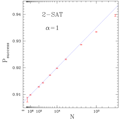
Figure 13: Numerical estimates of the probability of satisfiability of critical ($\alpha=1$) random 2-SAT formulas for different sizes $N$, plotted vs. $N^{-1/3}$. The straight line is a guess for the tangent to the curve at the point where it cuts the $N=\infty$ axis.

Appendix B Path-integral formalism for the kinetics of search

The standard, yet non-rigorous, technique of path integrals is another tool to study the search process. Let us re-derive some results of Sections 3 and 4.1 with it; this will show the correspondence between, on one hand, K-SAT related quantities and physical quantities such as moments, and, on the other hand, generating functions techniques and path-integral techniques, hopefully bringing more insights to both approaches.

We start from the evolution equation (7) and write the probability $P(T)$ that the search process doesn’t produce any 0-clause from times $0$ to $T$ as an iteration (this quantity was $G(0,1,1,\ldots,1;T)$ in Section 3):

$$\sum_{\vec{B}_{T}}P(\vec{B}_{T};T)=\sum_{\vec{B}_{T}}\sum_{\vec{B}_{T-1}}\ldots\sum_{\vec{B}_{1}}M(\vec{B}_{T}\leftarrow\vec{B}_{T-1};T-1)$$

$$\quad\times M(\vec{B}_{T-1}\leftarrow\vec{B}_{T-2};T-2)\times\ldots\times M(\vec{B}_{1}\leftarrow\vec{C}_{0};0)$$

$$=\sum_{\vec{C}_{1},\ldots,\vec{C}_{T-1}}\sum_{\vec{B}_{1},\ldots,\vec{B}_{T}}\int_{-\pi}^{\pi}\frac{d\vec{y}_{1}}{(2\pi)^{K}}\ldots\frac{d\vec{y}_{T}}{(2\pi)^{K}}\times$$ (B.139)

$$\quad\exp\left(\sum_{L=1}^{T}\hat{\imath}\vec{y}_{L}.(\vec{B}_{L}-\vec{C}_{L})\right)\prod_{L=0}^{T-1}M(\vec{B}_{L+1}\leftarrow\vec{C}_{L};L)$$

with $\vec{C}_{0}:=(0,0,\ldots,0,\alpha N)$ and $\hat{\imath}^{2}=-1$. All clause vectors are, in this Appendix, of dimension $K$ instead of $K+1$ since the number of 0-clauses is always zero. The $\vec{y}_{L}$’s constrain the $\vec{C}_{L}$’s to mimic the $\vec{B}_{L}$’s, so that we can write the formally quadratic expression $M(\vec{B}_{L+1}\leftarrow\vec{B}_{L};L)$ as the uncoupled expression $M(\vec{B}_{L+1}\leftarrow\vec{C}_{L};L)$. Carrying out the sums over the $\vec{B}_{L}$’s first, we obtain

$$P(T):=\sum_{\vec{B}_{T}}P(\vec{C}_{T};T)$$ (B.140)

$$\quad=\sum_{\vec{C}_{1},\ldots,\vec{C}_{T}}\int_{-\pi}^{\pi}\frac{\mathrm{d}\vec{y}_{1}}{(2\pi)^{K}}\ldots\frac{\mathrm{d}\vec{y}_{T}}{(2\pi)^{K}}\exp\left(-\sum_{L=1}^{T}\hat{\imath}\vec{y}_{L}.\vec{C}_{L}\right)$$

$$\qquad\times\exp\left(\sum_{L=0}^{T}\ln\left[\vec{f}(\vec{X}_{L};L)\right].\;\vec{C}_{L}\right)$$

$$\qquad\times\prod_{L=0}^{T}\bigg{[}(1-\delta_{(\vec{C}_{L})_{1},0})\;e^{-\hat{\imath}(\vec{y}_{L})_{1}}+\delta_{(\vec{C}_{L})_{1},0}\bigg{]}$$

where $(\vec{X}_{L})_{i}=\exp(\hat{\imath}(\vec{y}_{L})_{i})$, the vector-valued function $\vec{f}=(f_{1},f_{2},\ldots,f_{K})$ is defined through (12) and the dot denotes the usual scalar product of $\mathbb{R}^{K}$. In the large $N$ limit, a continuous formulation for $P(T)$ can be obtained. Let us define the reduced time, $\ell=L/N$ and the clause densities $\vec{c}(\ell)=\vec{C}(L)/N$. Define for $i=1,\ldots,K$

$$\gamma_{j}(\vec{y};t):=\frac{j}{1-t}\bigg{(}\frac{e^{-y_{j}}(1+e^{y_{j-1}})}{2}-1\bigg{)}$$ (B.141)

with $y_{0}:=-\infty$, and $\vec{\gamma}:=(\gamma_{1},\ldots,\gamma_{K})$. The probability $P$ at time $T=tN$ can be written as a path integral over the values of clause densities $\vec{c}$ and (from now on complex) ’momenta’ $\vec{y}$ between times 0 and $t$,

$$P(tN)=\int_{\vec{c}(0)=(0,0,\ldots,0,\alpha)}^{\vec{c}(t)=(c_{1},c_{2},\ldots,c_{K})}{\cal D}\vec{c}(\ell)\,{\cal D}{\vec{y}(\ell)}\times$$

$$\qquad\qquad\qquad\exp\bigg{(}-N\;{\cal S}\big{[}\{\vec{c}(\ell),\vec{y}(\ell)\}\big{]}\bigg{)}$$ (B.142)

where the action reads

$${\cal S}\big{[}\{\vec{c}(\ell),\vec{y}(\ell)\}\big{]} = \int_{0}^{t}d\ell\,\bigg{\{}\vec{y}(\ell).\frac{d\vec{c}}{d\ell}(\ell)-\vec{\gamma}\big{(}\vec{y}(\ell);\ell\big{)}.\vec{c}(\ell)$$ (B.143)

$$-\ln\big{[}\rho_{1}(\ell)\;e^{-y_{1}(\ell)}+1-\rho_{1}(\ell)\big{]}\bigg{\}}$$

where $\rho_{1}(\ell)$ denotes the probability that there is at least one unit clause at time $\ell$ i.e. the number of instants $L$ such that $C_{1}(L)\geq 1$ between $L=\ell N$ and $L=\ell N+\Delta L$, divided by $\Delta L$, with $1\ll\Delta L\ll L$. Minimization of the action (B.143) yields the classical equations of motion. Differentiating with respect to momenta, we find

$$\frac{\delta{\cal S}}{\delta y_{i}(\ell)}=0 \rightarrow \frac{dc_{i}}{d\ell}(\ell)=\sum_{j}\frac{\partial\gamma_{j}\big{(}\vec{y}(\ell);\ell\big{)}}{\partial y_{i}(\ell)}\;c_{j}(\ell)$$ (B.144)

$$\qquad-\frac{\delta_{i,1}\;\rho_{1}(\ell)}{\rho_{1}(\ell)+\big{(}1-\rho_{1}(\ell)\big{)}e^{y_{1}(\ell)}}\quad$$

for $i=1,\ldots,K$. Some care has to be brought to the minimization of the action with respect to the clause densities since $\rho_{1}$ and $c_{1}$ are not independent. During the time interval $[\ell,\ell+d\ell]$, the number $C_{1}$ of unit clauses is either of the order of $N$ ($c_{1}>0$ and $\rho_{1}=1$) or of the order of unity ($c_{1}=0$ and $\rho_{1}<1$) . With this caveat, we obtain

$$\frac{\delta{\cal S}}{\delta c_{i}(\ell)}=0\rightarrow\frac{dy_{i}}{d\ell}(\ell)=-\gamma_{i}\big{(}\vec{y}(\ell);\ell\big{)}\qquad(i=2,\ldots,K)$$ (B.145)

and

• if $c_{1}(\ell)>0$, then $\rho_{1}(\ell)=1$ and

  $$\frac{\delta{\cal S}}{\delta c_{1}(\ell)}=0\rightarrow\frac{dy_{1}}{d\ell}(\ell)=-\gamma_{1}\big{(}\vec{y}(\ell);\ell\big{)}$$ (B.146)

• if $c_{1}(\ell)=0$, then $\rho_{1}(\ell)$ is given by equation (B.144) for $i=1$,

  $$\frac{1}{\rho_{1}(\ell)}=1-e^{-y_{1}(\ell)}+e^{-y_{1}(\ell)}\bigg{(}\frac{\partial\gamma_{2}\big{(}\vec{y}(\ell);\ell\big{)}}{\partial y_{1}(\ell)}\;c_{2}(\ell)\bigg{)}^{-1}.$$ (B.147)

  Eq. (B.147) makes sense if the r.h.s. is larger than unity. In the case where $y_{1}=0$, it agrees with eq. (40).

Appendix C Large $t_{2}$-expansion of the solution $\rho$ of the PDE (77)

In this appendix we explain the method we used to get an asymptotic expansion of the solution of eq. (77) at large times $t_{2}$, and we quote the results. Eq. (77) is here treated in the general case $X_{0}\in[0,1]$ and reads

$$\partial_{t_{2}}\rho(c,t_{2})=\frac{1}{2}\partial_{c}^{2}\rho(c,t_{2})+\beta(p)t_{2}\partial_{c}\rho(c,t_{2})-\frac{1-X_{0}}{2}c\rho(c,t_{2})$$ (C.148)

First, we change the variables $c$ and $t$ for $u:=ct_{2}$ and $s:=1/t_{2}$ respectively, and define $g$ as $g(u,s):=\rho(c,t_{2})$. This is motivated by the expectation that, at large times $t_{2}$, both the drift term (that pushes diffusing particles towards the $c=0$ boundary) and the absorption term (that kills situations where many particles are away from the $c=0$ boundary) constrain the PDF $\rho$ to be concentrated around the $c=0$ boundary: $\rho(c,t_{2})$ will be non-vanishing only for values of $c$ that tend to 0 as $t\to+\infty$. With this choice of scale, eq. (C.148) turns at the leading order in $s$ when $s\to 0$ into

$$\partial_{u}^{2}g(u,s)+2\beta\partial_{u}g(u,s)=0$$ (C.149)

$$\partial_{u}g(0,s)+2\beta g(0,s)=0$$ (C.150)

hence $g(u,s)=A(s)\exp(-2\beta u)$: $c$ has at large times an exponential statistical distribution, with average (conditioned to success of the greedy algorithm) $\overline{c}(t_{2})=1/(2\beta t_{2})$.

To actually compute the normalization factor $A(s)$, we need to introduce formally the correction to this leading-order term. Let $\rho(c,t_{2})=:A(s)\exp(-2\beta u)+B(s)h(u,s)$ with the requirement $B(s)\ll A(s)$ as $s\to 0$. The leading-order terms in eq. (C.148) (after cancellation of the formerly leading-order terms) satisfy

$$\left[-2\beta suA(s)-s^{2}\partial_{s}A+us(1-X_{0})A(s)/2\right]\exp(-2\beta u)$$

$$\qquad=s^{-2}B(s)\left(\partial_{u}^{2}h+\beta\partial_{u}h\right)$$ (C.151)

with the boundary condition $\partial_{u}h(0,s)+2\beta h(0,s)=0$. This yields, after integration from $u=0$ to $+\infty$ (we assume that $h(u,s)\to 0$ when $u\to+\infty$ just like $\rho$ does),

$$A(s)\propto s^{-1+\frac{1-X_{0}}{4\beta}}$$ (C.152)

and, for the leading order of $\rho(c,t_{2})$ at large times:

$$\rho(c,t_{2})\propto t_{2}^{1-\frac{1-X_{0}}{4\beta}}\exp(-2\beta ct_{2}).$$ (C.153)

This shows that the probability of success of the algorithm decays algebraically at large times $t_{2}$:

$$\pi(0,t_{2})=\int_{c=0}^{+\infty}\rho(c,t_{2})\mathrm{d}c\quad\propto\quad t_{2}^{-\frac{1-X_{0}}{4\beta}}.$$ (C.154)

Subleading orders in the expansion of $\rho$ at large $t_{2}$ may be found iteratively by the same technique. For the sake of completeness, let us quote here what we found:

$$\rho(c,t_{2})\propto t_{2}^{1-(1-X_{0})/4/\beta}e^{-2\beta ct_{2}}\times$$ (C.155)

$$\quad\left[1+\left(1-\frac{1-X_{0}}{4\beta}\right)\left(c^{2}t_{2}^{2}-\frac{6\beta-1+X_{0}}{12\beta^{3}}\right)t_{2}^{-3}+\right.$$

$$\quad\ \left.\left(1-\frac{1-X_{0}}{4\beta}\right)\left\{\frac{c^{2}t_{2}^{2}}{48\beta^{4}}\left[(6\beta^{3}X_{0}+24\beta^{4}-6\beta^{3})c^{2}t_{2}^{2}+\right.\right.\right.$$

$$\left.\left.\left.\qquad\qquad\qquad\qquad\quad(48\beta^{3}+8\beta^{2}X_{0}-8\beta^{2})ct_{2}+\right.\right.\right.$$

$$\left.\left.\left.\qquad\qquad\qquad\ (-2\beta+2X_{0}\beta+2X_{0}+48\beta^{2}-1-X_{0}^{2})\right]\right.\right.$$

$$\left.\left.\qquad\qquad\qquad\qquad\quad-\frac{6\beta-1+X_{0}}{1152\beta^{7}}\times\right.\right.$$

$$\left.(384\beta^{2}-50\beta+50X_{0}\beta-1+2X_{0}-X_{0}^{2})\bigg{\}}t^{-6}+o(t^{-6})\right]$$

and, for the conditional average of $c$:

$$\overline{c}(t_{2})=\frac{1}{2\beta t_{2}}+\frac{4\beta-(1-X_{0})}{8\beta^{4}t_{2}^{4}}+$$ (C.156)

$$\quad\frac{5}{32\beta^{7}t_{2}^{7}}\left[4\beta-(1-X_{0})\right]\left[5\beta-(1-X_{0})\right]+o(\beta^{-7}t_{2}^{-7}).$$

Notice that the expansions here can only be asymptotic series, without a finite radius of convergence (as a function of $s=1/t_{2}$), because they are independent of the initial conditions. Indeed, fix $\epsilon>0$ and suppose that the sum of the expansion for $\rho$ above is the right solution, up to a uniform small difference $\epsilon$, on a finite interval of $t_{2}$, say $]A,+\infty[$. Let $\rho_{\mathrm{approx}}(c,t_{2})$ be this sum of the expansion. Then ask for the solution of eq. (77) that has initial condition $\rho(c,A+1)=\rho_{\mathrm{approx}}(c,A+1)+10\epsilon$: it should also be $\rho_{\mathrm{approx}}(c,A+1)$ up to a difference $\epsilon$ — contradiction! Therefore, the precision of the approximations obtained with partial sums of the expansion above decreases as we try to get values for smaller and smaller times $t_{2}$, and we should keep that in mind when we use the present results.

Appendix D Small $t_{2}$-expansion of the solution $\rho$ of the PDE (77)

In this Appendix we explain the method we used to get an asymptotic expansion of the solution of eq. (C.148) at small times $t_{2}$, and we quote the results.

We use the exact solution of eq. (C.148) without the non-linear term $c\rho(c,t_{2})$ (that is, for the special value $X_{0}=1$) as a guide for a relevant choice of variables. Disregarding the boundary condition eq. (79), we easily solve the resulting linear PDE thanks to Fourier transform:

$$\rho_{\mathrm{linear}}(c,t_{2})=\frac{\mathrm{constant}}{\sqrt{t_{2}-t_{2\mathrm{init}}}}\times$$ (D.157)

$$\quad\exp\left\{-\frac{1}{2(t_{2}-t_{2\mathrm{init}})}\left[c+\frac{\beta(p)}{2}(t_{2}^{2}-t_{2\mathrm{init}}^{2})\right]^{2}\right\}$$

which suggests us to use the following variables for our expansion:

$$v:=t_{2}-t_{2\mathrm{init}},\quad u:=\frac{c+\beta(p)/2(t_{2}^{2}-t_{2\mathrm{init}}^{2})}{\sqrt{t_{2}-t_{2\mathrm{init}}}},$$

$$\rho(c,t_{2})=:\frac{1}{\sqrt{v}}g(u,v)\ .$$

The equations for $g$ are

$$2v\partial_{v}g=\partial_{u}^{2}g+u\partial_{u}g+$$ (D.158)

$$\quad\left[1-(1-X_{0})v^{3/2}u+(1-X_{0})\beta(p)/2v^{2}(2t_{2\mathrm{init}}+v)\right]$$

$$\partial_{u}g[\beta(p)/2\sqrt{v}(2t_{2\mathrm{init}}+v),v]=$$ (D.159)

$$\quad-2\beta(p)\sqrt{v}(t_{2\mathrm{init}}+v)g[\beta(p)/2\sqrt{v}(2t_{2\mathrm{init}}+v),v]$$

At $t_{2}=t_{2\mathrm{init}}$, i.e. at $v=0$, $g$ is Gaussian, as expected from the study of the linear equation (with $X_{0}=1$): $g(u,0)=\sqrt{2\pi^{-1}}\exp(-u^{2}/2)$. Letting $v^{\gamma}h(u,v)$ be the deviation, at positive times $v$, between the exact $g$ and this Gaussian expression, and substituting this into the equations for $g$, we see that the boundary condition constrains $\gamma$ to the value $1/2$, and we are led to the ODE for $h(u,0)$

$$\partial_{u}^{2}h(u,0)+u\partial_{u}h(u,0)=0$$ (D.160)

with boundary condition $\partial_{u}h(0,0)=-2\beta(p)t_{2\mathrm{init}}/\sqrt{2\pi}$. Adding the physical requirement that $h(u,0)\to 0$ as $u\to+\infty$, we find the unique solution $h(u,0)=\beta(p)t_{2\mathrm{init}}[1-\mathrm{erf}(u/\sqrt{2})]$. Going on with this iterative process, we find that $\rho(c,v=t_{2}-t_{2\mathrm{init}})$ has the following expansion at small $v$:

$$\rho(c,v)=\sqrt{\frac{2}{\pi v}}\exp\left[-\frac{(c+\beta vw)^{2}}{2v}\right]\bigg{[}1+2\beta^{2}t_{2\mathrm{init}}^{2}v$$ (D.161)

$$\left.\quad-v(c+\beta vw)\left(\frac{3\beta}{4}+\frac{1-X_{0}}{8}+2\beta^{3}t_{2\mathrm{init}}^{3}\right)+o(v)\right]+$$

$$\quad\left(1-\mathrm{erf}\frac{c+\beta vw}{\sqrt{2v}}\right)\bigg{\{}\beta t_{2\mathrm{init}}-2\beta^{2}t_{2\mathrm{init}}^{2}(c+\beta vw)+$$

$$\quad v\left(\frac{3\beta}{4}-\frac{1-X_{0}}{8}+2\beta^{3}t_{2\mathrm{init}}^{3}\right)\left[\frac{(c+\beta vw)^{2}}{v}+1\right]$$

$$\qquad\qquad\qquad\qquad\qquad+o(v)\bigg{\}}$$

where $w$ stands for $(2t_{2\mathrm{init}}+v)/2$. Hence the expression for the conditional average of $c$:

$$\overline{c}(t_{2}) = \sqrt{\frac{2}{\pi}}\sqrt{t_{2}-t_{2\mathrm{init}}}-\frac{\beta(p)}{2}t_{2\mathrm{init}}(t_{2}-t_{2\mathrm{init}})$$

$$+\frac{\beta(p)^{2}}{6}\sqrt{\frac{2}{\pi}}t_{2\mathrm{init}}^{2}(t_{2}-t_{2\mathrm{init}})^{3/2}$$

$$+(t_{2}-t_{2\mathrm{init}})^{2}\left[\frac{9(1-X_{0})+10\beta(p)}{32}\right.$$

$$\qquad\left.-\frac{2}{3\pi}(1-X_{0})\right]+\mathcal{O}\left[(t_{2}-t_{2\mathrm{init}})^{5/2}\right].$$

Appendix E Direct numerical solution of the evolution equation (34) for the generating function $G_{1}$

For limited sizes $N$ of the problem, eq. (34) may be solved directly, with exact or high precision computer arithmetic. It may be used to compute the probability of success of the greedy algorithm from time steps 0 to $T$, $G_{1}(1,T)$ or the distribution of $C_{1}$ from the generating function $G_{1}$.

We assume that $X_{0}=0$ and that $C_{2}$ is known (from e.g. Eq. (29)). At $T=N$, $C_{1}$ is either 1 or 0 and a useful set of values of $X_{1}$ in eq. (34) is ${0,1}$ only. To compute $G_{1}(X_{1},N)$ with $X_{1}=0$ or 1, it is enough to know $G_{1}(X_{1},N-1)$ with $X_{1}=0$, $1/2$ or 1 after eq. (12) (we set $X_{0}=0$). This in turns requires successively the values $G(X_{1},T)$ for all $X_{1}\in{0,1/[2(N-T)],1/(N-T),\ldots,1}$. Starting from the known initial condition $G(X_{1},0)=1$, it is possible to compute iteratively, from $T=0$ to $N$, all values $G(k/[2(N-T)],T)$ for $0\leq k\leq 2(N-T)$ (at each step, only $2(N-T)+1$ numbers are stored). In practice, getting accurate results requires either doing exact arithmetics (which may be quite slow and/or memory consuming) or working with high precision floating point arithmetic (roughly speaking, the number of decimals digits has to be equal to $N$). This limited the range of $N$ to a few hundreds on the computer we used (2.4GHz Pentium IV processor with 1GB of RAM).

Using rounded, integer values for $C_{2}$ rather than simply $N\times c_{2}$ from eq. (29) makes computations much faster. In the case where exact arithmetic is used, it is needed to manage only rational numbers. For $N$ large enough, it brings only a small error on $G_{1}$.

If the number of 1-clauses at time $T$ is bounded by $2(N-T)$, $C_{1}$ is a polynomial of degree at most $2(N-T)$. Knowing its $2(N-T)+1$ values $G(k/[2(N-T)],T)$ is enough to compute it: $G_{1}$ may be expressed as a weighted sum of Lagrange interpolating polynomials. Finally, the coefficients of $G_{1}(X_{1})$ indicate the probability law of $C_{1}$. We used this technique to get the numerical results for the distribution of $C_{1}$ for 2-SAT with $N=501$ that are plotted in Figure (8). Contrary to estimates based on runs of the very algorithms under study, it doesn’t require averaging over many series since there is no randomness in the computation.

References

- (1) B. Aspvall, M. F. Plass, and R. E. Tarjan. A linear-time algorithm for testing the truth of certain quantified boolean formulas. Inf. Process. Lett., 8:121–123, 1979.
- (2) C. Papadimitriou and K. Steiglitz. Combinatorial Optimization. Dover, 1998.
- (3) John Franco. Probabilistic analysis of the pure literal heuristic for the satisfiability problem. Annals of Operations Research, 1:273–289, 1984.
- (4) John Franco and R. P. Swaminathan. Average case results for satisfiability algorithms under the random clause model. Annals of Mathematics and Artificial Intelligence, 20:357–391, 1997.
- (5) Ming-Te Chao and John Franco. Probabilistic analysis of a generalization of the unit-clause literal selection heuristics for the k-satisfiability problem. Inform. Sci., 51(3):289–314, 1990.
- (6) Dimitris Achlioptas. Lower bounds for random 3-sat via differential equations. Theor. Comp. Sci., 265(1–2):159–185, 2001.
- (7) Ming-Te Chao and John Franco. Probabilistic analysis of two heuristics for the 3-satisfiability problem. SIAM J. Comput., 15(4):1106–1118, 1986.
- (8) Alan Frieze and Stephen Suen. Analysis of two simple heuristics on a random instance of k-sat. J. Algorithms, 20(2):312–355, 1996.
- (9) Christophe Deroulers and Rémi Monasson. Critical behaviour of combinatorial search algorithms, and the unitary-propagation universality class. Europhys. Lett., 68(1):153–159, October 2004, cond-mat/0405319.
- (10) Rémi Monasson, Riccardo Zecchina, Scott Kirkpatrick, Bart Selman, and L. Toyansky. Phase transition and search cost in the 2+-sat problem. In 4th Workshop on Physics and Computation, Boston University, November 1996.
- (11) Scott Kirkpatrick and Bart Selman. Critical behavior in the satisfiability of random boolean expressions. Science, 264:1297–1301, 1994.
- (12) Bart Selman and Scott Kirkpatrick. Critical behavior in the computational cost of satisfiability testing. Artificial Intelligence, 81:273–295, 1996.
- (13) Dimitris Achlioptas, Lefteris M. Kirousis, Evangelos Kranakis, and Danny Krizanc. Rigorous results for random -sat. Theor. Comp. Sci., 265(1–2):109–129, 2001.
- (14) Olivier Dubois, Yacine Boufkhad, and Jacques Mandler. Typical random 3-sat formulae and the satisfiability threshold. In Proc. 11th ACM-SIAM Symposium on Discrete Algorithms, pages 126–127, 2000.
- (15) Alexis C. Kaporis, Lefteris M. Kirousis, and Efthimios G. Lalas. The probability analysis of a greedy satisfiability algorithm. In Proc. 10th Ann. European Symp. on Algorithms, pages 574–585, 2002.
- (16) David B. Wilson. On the critical exponents of random -sat. Random Structures and Algorithms, 21(2):182–195, 2002, math.PR/0005136.
- (17) Béla Bollobás, Christian Borgs, Jennifer T. Chayes, Jeong Han Kim, and David Bruce Wilson. The scaling window of the 2-SAT transition. Random Structures and Algorithms, 18(3):201–256, 2001.
- (18) Haiou Shen and Hantao Zhang. An empirical study of max-2-sat phase transition. In Proc. of LICS’03 Workshop on Typical Case Complexity and Phase Transitions. Ottawa, Canada, June 2003, 2003.
- (19) M. Davis and H. Putnam. A computing procedure for quantification theory. J. ACM, 7:201–215, 1960.
- (20) Gilles Dequen and Olivier Dubois. kcnfs: an efficient solver for random k-sat formulae. Lecture Notes in Computer Science 2919, Theory an Applications of Satisfiability Testing, pages 486–501, 2004.
- (21) Dimitris Achlioptas and Gregory B. Sorkin. Optimal myopic algorithms for random 3-SAT. In IEEE Symposium on Foundations of Computer Science, pages 590–600, 2000.
- (22) Nicholas C. Wormald. Differential equations for random processes and random graphs. The Annals of Applied Probability, 5(4):1217–1235, November 1995.
- (23) J. R. Albright. Integrals of products of airy functions. J. Phys. A – Math. Gen., 10:485–490, April 1977.
- (24) Piet Groeneboom. Brownian motion with a parabolic drift and airy functions. Probability Theory and Related Fields, 81:79–109, February 1989.
- (25) Milton Abramowitz and Irene A. Stegun. Handbook of Mathematical Functions with Formulas, Graphs, and Mathematical Tables. Dover, New York, ninth dover printing, tenth gpo printing edition, 1964.
- (26) Harris J. Silverstone, Sachiko Nakai, and Jonathan G. Harris. Observations on the summability of confluent hypergeometric functions and on semiclassical quantum mechanics. Phys. Rev. A, 32:1341–1345, September 1985.
- (27) Rémi Monasson and Riccardo Zecchina. Statistical mechanics of the random k-sat model. Phys. Rev. E, 56(2):1357–1370, August 1997, cond-mat/9606215.
- (28) Johan Håstad. Some optimal inapproximability results. In STOC ’97: Proceedings of the twenty-ninth annual ACM symposium on Theory of computing, pages 1–10, New York, NY, USA, 1997. ACM Press.
- (29) Johan Håstad. Some optimal inapproximability results. J. ACM, 48(4):798–859, July 2001.
- (30) S. Janson, T. Łuczak, and A. Rucinski. Random Graphs. Wiley, 2000.
- (31) M. E. J. Newman, S. H. Strogatz, and D. J. Watts. Random graphs with arbitrary degree distribution and their applications. Phys. Rev. E, 64:026118–1–17, July 2001.
- (32) Christina Goldschmidt. Critical random hypergraphs: the emergence of a giant set of identifiable vertices. Annals of Probability, 33(4):1573–1600, July 2005, math.PR/0401208.
- (33) D. Achlioptas and M. Molloy. The analysis of a list-coloring algorithm on a random graph. In FOCS ’97: Proceedings of the 38th Annual Symposium on Foundations of Computer Science (FOCS ’97), pages 204–212, Washington, DC, USA, 1997. IEEE Computer Society.
- (34) Liat Ein-Dor and Rémi Monasson. The dynamics of proving uncolourability of large random graphs. i. symmetric colouring heuristic. J. Phys. A – Math. Gen., 36:11055–11067, October 2003.
- (35) M. R. Garey and D. S. Johnson. Computers and Intractability: a guide to the theory of NP-completeness. W. H. Freeman and Co., New York, 1979.
- (36) Abdelaziz Amraoui, Andrea Montanari, Thomas J. Richardson, and Rüdiger L. Urbanke. Finite-length scaling for iteratively decoded ldpc ensembles. In Proc. 41th Annual Allerton Conference on Communication, Control and Computing, Monticello, IL, Oct 2003, 2004, cs.IT/0406050.