Secondary Structures in Long Compact Polymers

Abstract

Compact polymers are self-avoiding random walks which visit every site on a lattice. This polymer model is used widely for studying statistical problems inspired by protein folding. One difficulty with using compact polymers to perform numerical calculations is generating a sufficiently large number of randomly sampled configurations. We present a Monte-Carlo algorithm which uniformly samples compact polymer configurations in an efficient manner allowing investigations of chains much longer than previously studied. Chain configurations generated by the algorithm are used to compute statistics of secondary structures in compact polymers. We determine the fraction of monomers participating in secondary structures, and show that it is self averaging in the long chain limit and strictly less than one. Comparison with results for lattice models of open polymer chains shows that compact chains are significantly more likely to form secondary structure.

I Introduction

Proteins are long, flexible chains of amino acids which can assume, in the presence of a denaturant, an astronomically large number of open conformations. Twenty different types of amino acids are found in naturally occurring proteins, and their sequence along the chain defines the primary structure of the protein. The native, folded state of the protein contains secondary structures such as $\alpha$-helices and $\beta$-sheets which are in turn arranged to form the larger tertiary structures. Under proper solvent conditions most proteins will fold into a unique native conformation which is determined by its sequence. One of the goals of protein folding research is to determine exactly how the folded state results from the specific sequence of amino acids in the primary structure.

A number of theories exist to describe the forces that are responsible for protein folding Dill et al. (1995). Since there are many fewer compact polymer conformations than non-compact ones, entropic forces resist the tight packing of globular proteins. Tight packing is primarily the result of hydrophobic interactions between the amino acid monomers and the solvent molecules around them. Compared to the local forces between neighboring monomers along the chain, the hydrophobic interactions were historically seen as nonlocal forces contributing to the collapse process, but not responsible for determining the specific form of the native structure Anfinsen and Scheraga (1975).

This view has been challenged by ideas from polymer physics Dill (1999); Yee et al. (1994). In particular, polymers with hydrophobic monomers when placed in a polar solvent like water will collapse to a configuration where the hydrophobic residues are protected from the solvent in the core of the collapsed structure. Similarly, protein folding can be viewed as polymer collapse driven by hydrophobicity. The question then arises, how much of the observed secondary structure is a result of this non-specific collapse process?

To examine the role of hydrophobic interactions in folding, coarse-grained models of proteins have been developed, which reduce the 20 possible amino acid monomers to two types: hydrophobic (H) and polar (P). Further simplification is affected by using random walks on two or three dimensional lattices to represent chain conformations. Vertices of the lattice visited by the walk are identified with monomers, which in the HP model are of the H or P variety. Furthermore, in order to capture the compact nature of the folded protein state, Hamiltonian walks are often used for chain conformations. The Hamiltonian walk (or “compact polymer”) is a self-avoiding walk on a lattice that visits all the lattice sites. The compact polymer model was first used by Flory Flory (1956) in studies of polymer melting, and was later introduced by Dill Dill (1999) in the context of protein folding. The HP model provides a simple model within which a variety of questions regarding the relation of the space of sequences (ordered lists of H and P monomers) to the space of protein conformations (Hamiltonian walks) can be addressed; for a recent example see Ref. Li et al. (1996).

One of the first questions to be examined within the compact polymer model was to what extent is the observed secondary structure of globular proteins (i.e., the appearance of well ordered helices and sheets) simply the result of the compact nature of their native states. Complete enumerations of compact polymers with lengths up to 36 monomers found a large average fraction of monomers participating in secondary structure Chan and Dill (1989). This added weight to the argument that the observed secondary structure in proteins is simply a result of hydrophobic collapse to the compact state. This simple view was later challenged by off-lattice simulations, which showed that specific local interactions among monomers are necessary in order to produce protein-like helices and sheets Socci et al. (1994).

Here we reexamine the question of secondary structure in compact polymers on the square lattice using Monte-Carlo sampling of the configuration space. We compute the probability of a monomer participating in secondary structure in the limit of very long chains. We show that this probability is strictly less than one, and that it depends on the precise definition of secondary structure in the lattice model. We also show that, in the long-chain limit, compact polymers are much more likely to exhibit secondary structure motifs than their non-compact counterparts, such as ideal chains, described by random walks, or polymers in a good solvent, modelled by self-avoiding random walks. The Monte-Carlo technique described below can be easily extended to three-dimensional lattices and other models (such as the HP model) that make use of Hamiltonian walks. In a forthcoming paper we further demonstrate its utility in the context of the Flory model of polymer melting Oberdorf et al. .

Hamiltonian walks on different lattices are also interesting statistical mechanics models in their own right, as their scaling properties give rise to new universality classes of polymers. An unusual property of these walks is that different lattices do not necessarily lead to the same universality class. This lattice dependence is linked to geometric frustration that results from the constraint that Hamilton walks must visit all the sites of the lattice. In addition, compact polymers can be obtained as the zero-fugacity limit of fully packed loop models (the exact form of which depends on the lattice) allowing for the exact calculation of critical exponents Jacobsen and Kondev (1998).

Numerical investigations of compact polymers are typically hampered by the need to generate a sufficient number of statistically independent compact configurations for the construction of a suitable ensemble. It is not hard to see that attempting to generate compact structures by constructing self-avoiding random walks on a lattice would indeed be a problematic endeavor; current state-of-the-art algorithms are essentially “smarter” chain growth strategies where the next step in the random walk is taken based on not only the self-avoidance constraint but on a sampling probability which improves as the program proceeds J. Zhang et al. (2003). Enumerations of all possible states have been performed for both regular self-avoiding random walks J. Liang et al. (2002) and for compact polymers Camacho and Thirumalai (1993), but this has only been possible for small lattices ($N<36$). Therefore, an algorithm which can rapidly generate compact configurations on significantly larger lattices, without the complication of constructing advanced sampling probabilities would be an extremely useful tool.

In Ref. jernigan a method for generating compact polymers based on the transfer matrix method was introduced. One limitation of the method is that the transfer matrices become prohibitively large as the number of sites in the direction perpendicular to the transfer direction increases above 10. A very efficient Monte-Carlo method based on a graph theoretical approach was introduced in caruthers and improved on in Lua et al. (2004) by reducing the sampling bias.

One of the purposes of this paper is to describe a Monte-Carlo method for efficiently generating compact polymer configurations on the square lattice for chain lengths up to $N=2500$. The Monte-Carlo algorithm outlined below makes use of the “back bite” move, which was first introduced by Mansfield in studies of polymer melts Mansfield (1982). We perform a number of measurements to assess the validity and practicality of the algorithm for generating compact polymer configurations. Probably the most important and certainly the most elusive property is that of ergodicity, which would guarantee that the algorithm can sample all compact polymer configurations. While we have been unsuccessful in constructing a proof of ergodicity, we find excellent numerical evidence for it based on a number of different tests. In particular, we check that the measured probability that the polymer endpoints are adjacent on the lattice is in agreement with exact enumeration results for polymer chain lengths up to $N=196$. Furthermore, we demonstrate that the Monte-Carlo process satisfies detailed balance, which guarantees, at least in the theoretical limit of infinitely long runs, that the sampling is unbiased. We check this in practice with a quantitative test of sampling bias for $N=36$ (ie. for compact polymers on a $6\times 6$ square lattice).

For the Monte-Carlo process to be useful it should also sample the space of compact polymer configurations efficiently. To quantify this property of the algorithm, we measure the processing time required to generate a fixed number of compact polymer conformations, and find it to be linear in chain length $N$. Since the sampling is of the Monte-Carlo variety a certain number of Monte-Carlo steps need to be performed before the initial and the final structure can be deemed statistically independent. We find that this correlation time, measured in Monte-Carlo steps per monomer, grows with chain length as $N^{z}$ with $z\approx 0.16$.

We put the Monte-Carlo algorithm to good use by tackling the question of the statistics of secondary structure in compact polymer chains. While the previous study by Chan and Dill Chan and Dill (1989) found a large fraction of monomers participating in secondary-structure motifs, the polymer physics question of what happens to this quantity in the long-chain limit, remained unanswered. Based on exact enumerations for chain lengths up to $N=36$ the hypothesis that was put forward was that in the long chain limit almost all the monomers will participate in secondary structure. Our computations on the other hand, show that the probability of a monomer participating in secondary structure tends to a fixed number strictly less than one. Furthermore the actual number depends on the precise definitions used for secondary structure motifs. Still, from gathered statistics on the appearance of helix-like motifs in simple random walks and self-avoiding walks, we conclude that the propensity for secondary structures in compact polymers is much greater than in their non-compact counterparts, even in the long chain limit. This provides further support for the idea that the global constraint of compactness, imposed on globular proteins by hydrophobicity, favors formation of secondary structure.

The paper is organized as follows. In section II we describe our Monte-Carlo process for sampling compact polymers, which is based on Mansfield’s backbite move Mansfield (1982). The correctness and usefulness of the Monte-Carlo algorithm for sampling compact polymer configurations, is evaluated in section II.1. Finally, in section III we give details of our computations of secondary structure statistics for compact polymers with lengths ranging from $N=36$ to $N=2500$. The main conclusion of this section is that the fraction of monomers participating in secondary structures is Gaussian distributed with a variance that vanishes in the long-chain limit. Its mean is strictly less than one but still more than twice as large as the values measured for non-compact lattice models of polymers.

II Monte-Carlo sampling of compact polymers

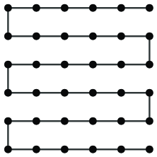
Figure 1: Compact polymer configuration on a $6\times 6$ lattice. This “plough” configuration is used as the initial state for the Monte-Carlo process.

The Monte Carlo process starts with an initial Hamiltonian walk on the lattice. We use a square lattice with side $\sqrt{N}$, $N$ being the polymer length. The initial walk is the “plough” shown in Fig. 1. Starting from this initial compact polymer configuration, new configurations are generated by repeatedly applying the backbite move Mansfield (1982). Namely, given a Hamiltonian walk (Fig. 2a), a link is added between one of the walk’s free ends and one of the lattice sites adjacent, but not connected, to that end. This adjacent site is chosen at random with each possible site having an equal probability of being chosen (Fig. 2b). After the new link has been added we no longer have a valid Hamiltonian walk, since three links are now incident to the chosen site. To correct this we remove one of the three links, which is uniquely characterized by being part of a cycle (closed path) and not being the link just added (Fig. 2c). After one iteration of this process one of the ends of the walk has moved two lattice spacings, and a new Hamiltonian walk has been constructed (Fig. 2d).

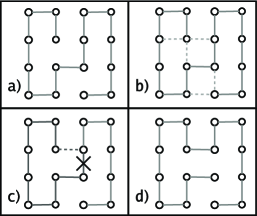
Figure 2: Illustration of the “backbite” move used to generate a new Hamiltonian walk from an initial one. Starting from a valid walk a), one additional step is made starting at either of the two ends of the walk, b). Next we delete a step, shown in c), to produce a new valid walk, d).

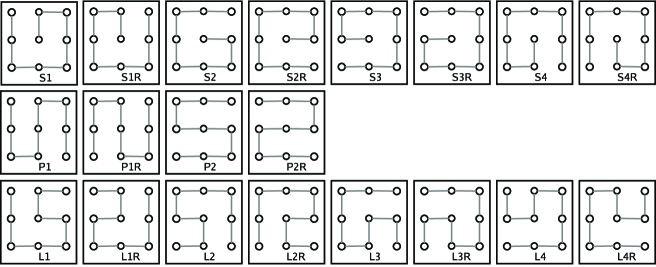
Figure 3: Enumeration of all possible Hamiltonian walks on a $3\times 3$ square lattice.

By repeatedly executing the backbite move it seems that all possible Hamiltonian walks are generated. To examine this statement more closely, we first consider compact polymers on a $3\times 3$ lattice. Fig. 3 shows an enumeration of all possible compact polymer configurations on this lattice. The corresponding walks may be divided into three classes where all the walks in a given class (Plough, Spiral or Locomotive—denoted P, S and L in the figure) are related by reflection (denoted R in the figure) and/or rotation. (Note that P-class walks are invariant under rotation by 180 degrees, and that there are half as many P-class walks as S or L-class walks.) Fig. 4 shows the transition graph that connects compact polymer configurations on a $3\times 3$ lattice that are related by a single backbite move. We see that all the 20 possible walks can be reached from any initial walk. Furthermore, it is important to notice that the S-class walks have four moves leading in and out of them, while the L and P-class walks only have two moves leading in and out of them. This happens as a result of the locations of a walk’s end points. Namely, on a square lattice an end point on a corner can only be linked to one adjacent site by the backbite move, end points on the edges can be linked to two sites, while end points in the interior of the lattice can be linked to three sites. Because there are twice as many moves leading to S-class walks as there are for P-class or L-class, the S-class walks are twice as likely to be generated if backbite moves are repeatedly performed (this subtlety is absent if periodic boundary conditions are employed).

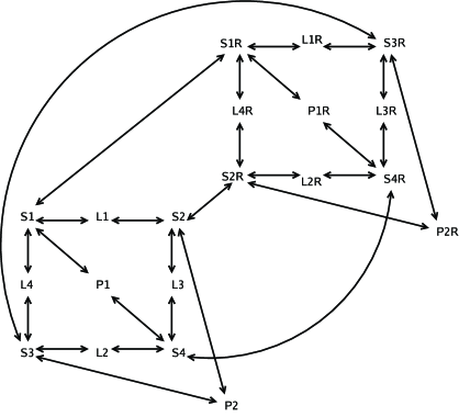
Figure 4: Transition graph for compact polymers on the $3\times 3$ square lattice generated by the backbite move.

In order to compensate for this source of bias in sampling of compact polymers, an adjustment to the original process is made: for structures which have fewer paths available to access them, we introduce the option of leaving the current walk unchanged in the next Monte-Carlo step. The probability of making a transformation from the current walk is calculated by counting how many links $l$ can be drawn from the end points of the current walk and dividing that number by the maximum number ($l_{\rm max}$) of links that could be drawn for any walk on the lattice. For example, consider a P-class walk on a $3\times 3$ lattice. There are two possible links that could be drawn from the end points of this walk, but there is a maximum of 4 links that could be drawn (which happens in the case of S-class walks). Thus the probability of making a backbite move is $\frac{l}{l_{\rm max}}=\frac{2}{4}=0.5$.

With this adjustment of the original Monte Carlo process, all walks accessible from the initial walk will occur with equal probability, upon repeating the algorithm a sufficiently large number of times. Technically speaking, the amended algorithm satisfies detailed balance. In general, the criterion for detailed balance reads $p_{\alpha}P(\alpha\to\alpha^{\prime})=p_{\alpha^{\prime}}P(\alpha^{\prime}\to\alpha)$, where $p_{\alpha}$ is the probability of the system being in the state $\alpha$, and $P(\alpha\to\alpha^{\prime})$ is the transition probability of going from the state $\alpha$ to another state $\alpha^{\prime}$. In thermal equilibrium one must have $p_{\alpha}=Z^{-1}\exp(-\beta E_{\alpha})$, where $\beta$ is the inverse temperature, $E_{\alpha}$ is the energy of the state $\alpha$, and $Z=\sum_{\alpha}\exp(-\beta E_{\alpha})$ is the partition function. In the problem at hand we have assigned the same energy (say, $E_{\alpha}=0$) to all states, whence the criterion for detailed balance reads simply $P(\alpha\to\alpha^{\prime})=P(\alpha^{\prime}\to\alpha)$.

Now suppose that the state $\alpha$ can make transitions to $l_{\alpha}$ other states. (In the above example, $l_{\alpha}=2$ for the P-class walks and $l_{\alpha}=4$ for the S-class walks.) Then we can choose $P(\alpha\to\alpha^{\prime})$ equal to $\pi(\alpha\to\alpha^{\prime})\equiv{\rm min}(1/l_{\alpha},1/l_{\alpha^{\prime}})$ for $\alpha\neq\alpha^{\prime}$. Define $\gamma(\alpha)=\sum^{\prime}_{\alpha^{\prime}}\pi(\alpha\to\alpha^{\prime})$, where the sum is over the $l_{\alpha}$ states $\alpha^{\prime}$ which can be reached by a single move from the state $\alpha$. In order to make sure that probabilities sum up to $1$, we must introduce the probability $P(\alpha\to\alpha)=1-\gamma(\alpha)$ for doing nothing. Better yet, we can eliminate the possibility of doing nothing by renormalizing the Monte-Carlo time. Namely, let the transition out of the state $\alpha$ correspond to a Monte-Carlo time $1/\gamma(\alpha)$ and pick the transition probabilities as $P(\alpha\to\alpha^{\prime})=\pi(\alpha\to\alpha^{\prime})/\gamma(\alpha)$. Then the transition rates (i.e., the transition probability per unit time) satisfies detailed balance as it should. This renormalized dynamics is clearly optimal in the sense that now the probability of leaving the state unchanged is zero, $P(\alpha\to\alpha)=0$. In practice, the optimal choice only presents an advantage if the numbers $l_{\alpha}$ are easy to evaluate (which is the case here) and if their values vary considerably with $\alpha$ (which is not the case here). Accordingly, we have used only the simpler $l/l_{\rm max}$ prescription described in the preceding paragraph.

Even though we have satisfied detailed balance, a walk generated by the Monte Carlo process does not immediately start occurring with a probability that is independent of the initial walk. For large $N$ in particular, a walk generated by the process will show a great deal of structural similarity to the walk that it was created from because only two links of the walk get changed in each iteration of the process. To work around this problem a large number of walks must be generated to yield the final ensemble. Below we address this important practical issue in great detail.

II.1 Properties of the Monte Carlo process

In evaluating the suitability of the Monte-Carlo algorithm for statistical studies of compact polymers the following issues must be addressed: 1. Does the process generate all possible Hamiltonian walks on a given lattice? 2. Is the sampling as described in the previous section truly unbiased? 3. How rapidly do descendant structures lose memory of the initial structure? 4. How does the processing time to generate a fixed number of walks scale with the number of lattice sites? The first two questions relate to issues of ergodicity and detailed balance which both need to be satisfied so that structures are sampled correctly. The last two questions pertain to the efficacy with which the algorithm can generate uncorrelated structures that can be used in computations of ensemble averages. Below we give detailed answers to these questions.

We have been unable to provide a general proof of ergodicity, i.e., that the Monte-Carlo process can generate all possible Hamiltonian walks on square lattices of arbitrary size. However, we have observed that the process successfully generates all of the possible walks on square lattices of size $3\times 3$, $4\times 4$, $5\times 5$, and $6\times 6$. It should be noted that for $5\times 5$ and $6\times 6$ lattices, all possible “combinations” of end point locations are possible, while on smaller lattices only walks with corner-corner, core-corner, and corner-edge combinations are allowed. Whether endpoints are on edges, corners, or in the bulk of the lattice is important because it determines how many links might be drawn from an endpoint which in turn determines the probability of making a Monte-Carlo step away from the current structure. Both $5\times 5$ and a $6\times 6$ lattices have $l_{\rm max}=6$, which is the largest possible $l_{\rm max}$ on the square lattice. In this sense, we consider these two lattices representative of larger lattices.

It should also be noted that the algorithm is likely to exhibit parity effects. This is linked to the fact that a square lattice can be divided into two sublattices (even and odd). Namely, on a lattice of $N$ sites, the two end points must necessarily reside on opposite (resp. equal) sublattices if $N$ is even (resp. odd). To see this, note that when moving along the walk from one end point to the other, the site parity must change exactly $N-1$ times. In particular, only when $N$ is even can the two end points be adjacent on the lattice. It is therefore reassuring to have tested ergodicity for both $5\times 5$ and $6\times 6$ lattices.

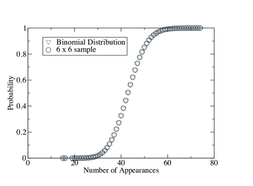
Figure 5: Comparison of sampling statistics of compact polymers on the $6\times 6$ lattice produced by the Monte Carlo process with the binomial distribution, which is to be expected for an unbiased sampling.

To test whether or not the process generates unbiased samples, $K=10^{7}$ compact polymer conformations were generated on a $6\times 6$ lattice. All different conformations were identified and the number of occurrences of each identified conformation was counted. The number of conformations on a $6\times 6$ lattice is known by exact enumeration to be $M=229\,348$ Jacobsen , and our algorithm indeed generates all of these. Using a method similar to the one used in Ref. Lua et al. (2004) we construct the histogram of the frequency with which each one of the $M$ possible conformations occurs. This histogram is then compared to the relevant binomial distribution. Namely, if each conformation occurs with equal probability $p=\frac{1}{N}$ then the probability of a given conformation occurring $k$ times in $K$ trials is $P(k)=\frac{K!}{k!(K-k)!}p^{k}(1-p)^{K-k}$. In Fig. 5 we compare $P(k)$ to the distribution constructed from the actual $6\times 6$ sample. A close correspondence between the predicted distribution and the distribution constructed from the Monte-Carlo data is evident from the figure, indicating no detectable sampling bias in this case.

$L$	$M_{0}/M_{1}$	$P_{1}^{\rm enum}$	$P_{1}^{\rm MC}$
2	$\frac{1}{4}$	1.00000000	1.0000
4	$\frac{6}{276}$	0.34782609	0.3455
6	$\frac{1072}{229348}$	0.16826831	0.1664
8	$\frac{4638576}{3023313284}$	0.09819322	0.0979
10	$\frac{467260456608}{730044829512632}$	0.06400435	0.0633
12	$\frac{1076226888605605706}{3452664855804347354220}$	0.04488610	0.0442
14	$\frac{56126499620491437281263608}{331809088406733654427925292528}$	0.03315399	0.0323

Table 1: The probability $P_{1}$ that the walk’s two end points are adjacent on an $L\times L$ lattice, as obtained by exact enumeration (see text) and by the Monte Carlo method.

Further evidence that the sampling is unbiased is provided by computing the probability $P_{1}$ that the end points of the generated walks are separated by one lattice spacing. Note that when this is the case, the walk could be turned into a closed walk, or Hamiltonian circuit, by adding a link that joins the two end points. Conversely, a closed walk on an $N$-site lattice can be turned into $N$ distinct open walks by removing any one of its $N$ links. Therefore $P_{1}=NM_{0}/M_{1}$, where $M_{0}$ (resp. $M_{1}$) is the number of closed (resp. open) walks that one can draw on the lattice. Using this formula, we can compare $P_{1}$ as obtained by the Monte Carlo method, to $P_{1}$ from exact enumeration data. The exact enumerations are done using a transfer-matrix method for lattice sizes up to $14\times 14$ Jacobsen . The results displayed in Table 1 show that the two determinations of $P_{1}$ are in excellent agreement.

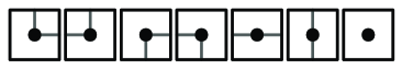
Figure 6: Possible path shapes through the vertex of a square lattice.

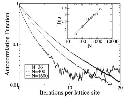
Figure 7: Autocorrelation curves for various polymer lengths, $N$. This inset shows the dependence of a characteristic time scale constant $\tau$, extracted from the autocorrelation curves, on polymer length $N$.

To quantify the rate at which descendant structures become decorrelated from an initial structure we must first devise a method for computing the similarity of two structures. The method used here is to compare, vertex by vertex, the different ways in which the walk can pass through a vertex. Looking at the examples of walks in Fig. 3 we immediately see that there are seven possibilities, shown in Fig. 6. The walk may move vertically or horizontally straight through a vertex, form a corner in four different ways, or terminate at a vertex. To evaluate the autocorrelation time, a walk is represented by $N$ variables $\sigma_{i}=1,2,\ldots,7$ that encode the possible shapes at each lattice site $i$. The similarity $S(\sigma,\sigma^{\prime})$ of two walks $\{\sigma_{i}\}$ and $\{\sigma^{\prime}_{i}\}$ is then defined as $S(\sigma,\sigma^{\prime})=N^{-1}\sum_{i}\delta_{\sigma_{i},\sigma^{\prime}_{i}}$. As the Monte-Carlo process progresses from an initial Hamiltonian walk we expect that the similarity between the initial and the descendent walks to decay with Monte-Carlo time. In order to estimate the characteristic time scale $\tau$ for this decay, we plot in Fig. 7 the autocorrelation function

$$A(t)=\frac{\left<S(\sigma(0),\sigma(t))\right>-\left<S\right>_{\rm min}}{1-\left<S\right>_{\rm min}}$$ (1)

where the average is taken over many runs and $\left<S\right>_{\rm min}$ is the smallest average similarity computed for the duration of the Monte-Carlo process, for a given $N$. The walk $\sigma(t)$ is one obtained after $t$ Monte-Carlo steps per lattice site applied to the initial walk $\sigma(0)$.

The curves in Fig. 7 have an initial, exponentially decaying regime. In this regime we fit them to the function $A\exp(-t/\tau)$ to obtain as estimate for the autocorrelation time $\tau$. The inset of Fig. 7 shows the dependence of $\tau$ on polymer length $N$, plotted on a log-log plot. Fitting now the polymer length dependence using $\tau=BN^{z}$, we get the estimate $z=0.16\pm 0.03$ for the dynamical exponent. The fact that the dynamical exponent is small tells us that increasing the polymer length in the simulation will not lead to a large increase in computational cost.

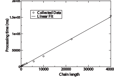
Figure 8: Effect of varying the compact polymer length on processing time required to generate $10^{6}$ consecutive structures by the Monte-Carlo process. Computations were performed on a 500 Mhz Pentium III computer with 512 megabytes of RAM.

There are two ways in which polymer length plays a role in the performance of the algorithm described above. First, measurements show that the processor time needed to generate a fixed number of walks scales linearly with their length (see Fig. 8). However, this particular result only considers the time to generate a fixed number of consecutive structures in the Monte-Carlo process, which, as we have seen, are not statistically independent. The actual processing time to generate an ensemble of properly sampled structures would increase the reported times by a factor equal to the number of iterations needed to achieve statistical independence of samples. This factor roughly equals the autocorrelation time $\tau$, which depends on $N$ through the exponent $z$ determined above.

III Secondary structures in compact polymers

The presence of secondary structure-like motifs in compact polymers on the square lattice has been extensively studied for chain lengths up to $N=36$ Chan and Dill (1989). It was shown in Ref. Chan and Dill (1989) that it is very unlikely to find a compact chain with less than 50% of its residues participating in secondary structures and that the fraction of residues in secondary structures increases as the chain length increases. Based on studies of chains up to $N=36$ it appeared that the fraction of participating residues would asymptotically approach 100% as $N$ increased. Using the Monte-Carlo approach described above we have extended these calculations to $N=2500$ and find that the fraction of residues participating in secondary structures, in the long-chain limit, tends to a number strictly less than one. We also show that this number is definition dependent but is still substantially greater for compact polymers than for non-compact chains.

III.1 Identification of secondary structures

There is more than one way to identify secondary structures in lattice models of proteins. Following Ref. Chan and Dill (1989) we make use of contact maps which provide a convenient and general way of representing secondary structure motifs. A contact map is a matrix of ones and zeroes, where the ones represent those pairs of residues which are adjacent on the lattice, but not connected along the chain. In this representation secondary structures are identified by searching for patterns in the contact map which represent helices, sheets, and turns; an example is shown in Fig. 9.

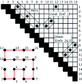
Figure 9: Contact map for a Hamiltonian walk on a $4\times 4$ square lattice. A filled circle in position $(i,j)$ indicates that residues $i$ and $j$ are in “contact”; they are adjacent on the lattice but are not nearest neighbors along the chain. Secondary structure motifs defined in Fig. 10 appear as distinct patterns in the contact map.

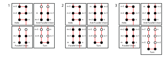
Figure 10: Three definitions used to identify secondary structures in compact polymers. The shaded vertices (monomers) are counted as participating in the particular secondary structure motif. Definition 1 is the most liberal while 3 is the most conservative. Definitions 1 and 2 are identical to those used in Ref. Chan and Dill (1989). The rationale for definition 3 is described in the text.

In order to test the generality of our findings, data was collected using three different sets of definitions for secondary structure which are illustrated in Fig. 10. Since there is no unique definition of secondary structure for lattice models of proteins, these models can at best provide qualitative answers to questions relating to real proteins, like the role of hydrophobic collapse in secondary structure formation. In other words, any conclusions derived from the lattice model which might hope to apply to real proteins should certainly not depend on the particular definition employed.

The first definition summarized in Fig. 10 is the least restrictive one. Because sheets only require two pairs of adjacent residues, this definition allows for pairs of residues to participate in both helices and sheets. Unfortunately, this property does not have any counterpart in real proteins. For this reason, and following Ref. Chan and Dill (1989), we also implement a second definition for both parallel and anti-parallel sheets which requires them to have three pairs of adjacent monomers instead of just two. This makes it more difficult for a residue to be part of both a sheet and a helix. The third definition that we use, also shown in Fig. 10, is even more strict than the second definition: a turn now requires three pairs of residues to be in contact. This ensures that a turn can only be identified if it is part of a sheet, which was not necessarily the case in the second definition.

III.2 Statistics of secondary structures

To gather the statistics on secondary structure motifs, 50 000 statistically independent Hamiltonian walks on the square lattice were generated for chain lengths ranging between $N=36$ and $N=2500$. For each walk, the residues participating in secondary structure were identified and counted using each of the three sets of definitions. To determine the fraction of residues participating in secondary structure for a given walk, the count is then divided by $N$, the total number of residues. The histogram of the fraction of sites participating in secondary structure is subsequently constructed for each chain length.

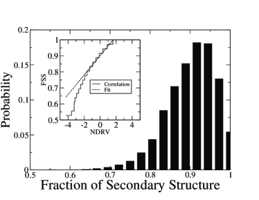
(a) Definition 1, N=36

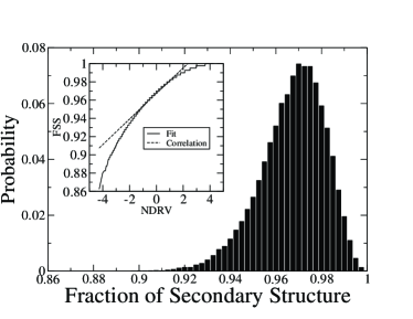
(b) Definition 1, N=400

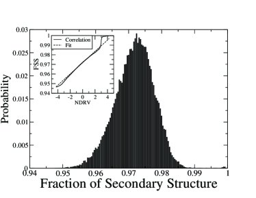
(c) Definition 1, N=2500

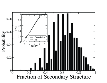
(d) Definition 2, N=36

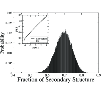
(e) Definition 2, N=400

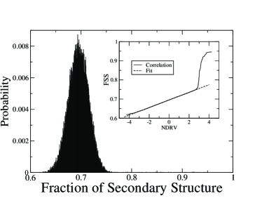
(f) Definition 2, N=2500

Figure 11: Probability distribution for the fraction of residues participating in secondary structure for varying polymer lengths. The figures show only the first two definitions of secondary structure represented in Fig. 10. The insets show the correlation between the measured distributions and a normally distributed random variable (NDRV). Straight lines indicate a strong correlation to the Gaussian distribution and the slopes of the lines reflect the distribution variances.

Plots of the histograms of the participation fraction are shown in Fig. 11 for definitions 1 and 2. Both the mean and the variance of the participation fraction clearly depends on the definition employed. As the polymer length $N$ increases the distributions appear to approach a Gaussian shape for all definitions, and they are more and more sharply peaked around the mean.

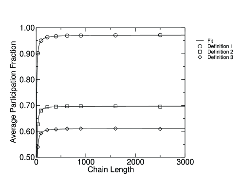
Figure 12: Average fraction of residues participating in secondary structure as a function of chain length $N$. The full lines represent a three-parameter fit to the function $f_{\infty}-a/N^{x}$.

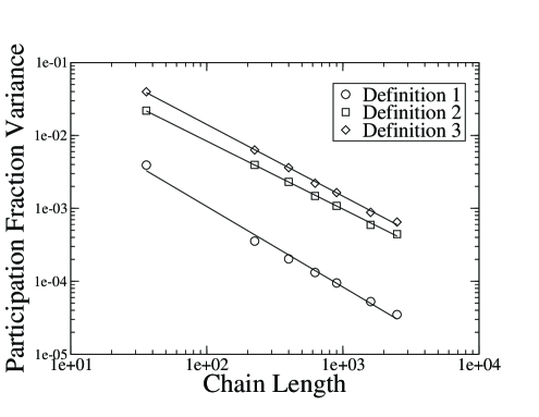
Figure 13: Variance of the participation fraction as a function of chain length for all three definitions of secondary structure.

From the measured participation fractions we compute their mean and variance. The dependence of the mean on the polymer length is shown in Fig. 12. As polymer length increases the average fraction of residues participating in secondary structure approaches a fixed number $f_{\infty}$, which clearly depends on the definition used. Although the definition affects the specific value of $f_{\infty}$, each curve has roughly the same shape which is well fit by the function $f=f_{\infty}-a/N^{x}$. In all cases the numerical value of $f_{\infty}$, the participation fraction in the long chain limit, is less than 1 (see Table 2).

Definition	$f_{\infty}$	$a$	$x$
1	0.9719	4.2511	1.1451
2	0.6972	11.7942	1.4303
3	0.6108	8.8789	1.3461

Table 2: The parameters obtained from fitting the average fraction of residues participating in secondary structures $f$ for different chain lengths $N$, to the functional form $f=f_{\infty}-a/N^{x}$.

The variance of the fraction of residues participating in secondary structure is shown in Fig. 13. It clearly decreases with $N$ in a power-law fashion. A linear fit on the log-log plot reveals that the variance scales as $1/N$, regardless of the definition of secondary structure employed. This result indicates that for compact polymers on the square lattice the fraction of residues participating in secondary structure has a well defined long chain limit given by $f_{\infty}$.

In order to quantify how closely the histograms in Fig. 11 approach a Gaussian distribution, the percent of residues participating in secondary structure is plotted against a normally distributed random variable. These plots appear as insets in Fig. 11, and a straight line indicates a Gaussian distribution. Note that deviations from a straight line appear in the tails of the distributions. We attribute this primarily to the influence of the initial “plough” configuration on the sampled walks. This we verified by comparing histograms for the participation fraction constructed from three different ensembles of compact polymers which differed by the number of Monte-Carlo steps taken before sampling is initiated. As the initial wait time for the sampling to commence is increased we find that the deviations from the Gaussian distribution decrease. In fact, in order to lose memory of the initial plough state, we found the wait time to be of the order of $10\tau$, where $\tau$ is the measured correlation time.

In order to understand the degree to which global compactness, as opposed to local connectivity, of the chains is responsible for the formation of helices we investigated the set of all $2\times 3$ motifs that can be observed in a compact polymer configuration. Namely, on a $2\times 3$ section of square lattice there are 7 possible bonds that can be drawn, which means there are $2^{7}$ different $2\times 3$ motifs. Of course, not all of these are compatible with a compact polymer configuration. For example, motifs with all bonds present or no bonds present could not be part of a valid Hamiltonian walk. In fact we found 67 allowed motifs, of which only two are helices. Therefore, the naive assumption that each of the allowed motifs appears with an equal probability would lead to the expectation of only 3% of residues participating in helix motifs. By comparison, simulations of long chains place the expected value near 28%.

To further assess the importance of being compact for the emergence of secondary structures, we generated ensembles of random walks and self-avoiding random walks and compared their helix-content to that of Hamiltonian walks. Random walks were generated simply from a series of random steps on the square lattice. Self-avoiding walks were sampled using a Monte-Carlo process based on the pivot algorithm Gaylord and Wellin (1995). The results of these computations are shown in Fig. 14.

a)

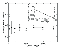
b)

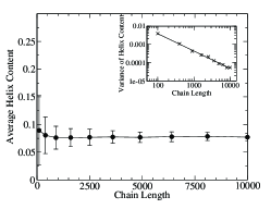
c)

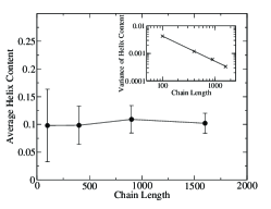
Figure 14: Average fraction of residues participating in helices for a) Hamiltonian walks, b) random walks and c) self-avoiding random walks. The insets show the variance of the helix content as a function of the chain length.

As might be expected, based on the results stated above, the measured helix content is self averaging (its distribution becomes narrower with increasing $N$), for all three polymer models. This is explicitly seen in the insets in Fig. 14 where we plot the variance of the fractional helix content distribution. We find that there is a clear difference in the average helical content of random walks and self-avoiding walks compared to Hamiltonian walks. The three different polymer models have 8%, 11%, and 28% helical content, respectively, in the long chain limit.

IV Conclusion

In this paper we describe and test a Monte-Carlo algorithm for sampling compact polymers on the square lattice. The algorithm is based on the “backbite” move introduced by Mansfield Mansfield (1982) for the purpose of simulating a many-chain polymer melt. We demonstrate that the algorithm satisfies detailed balance which ensures that all the accessible states are sampled with the correct weight. While we have been unable to prove the ergodicity of the algorithm for large lattice sizes a number of numerical tests seem to indicate its validity. Furthermore, we measure the efficacy of the algorithm and find that the computational effort (measured in Monte-Carlo steps per site) grows slightly faster than linear with the polymer length. In practice, using a pentium-based workstation, it takes roughly an hour to sample 10000 statistically independent compact polymer configurations for a chain 2500 monomers in length.

We employ this algorithm in studies of secondary structure of compact polymers on the square lattice, in the long chain limit. Our results complement the results found previously for short chains by Chan and Dill Chan and Dill (1989). Namely, we show that the fraction of residues participating in secondary structure has a well defined long-chain limit that is strictly less than one. Looking at helix content alone, we find that helices are twice as likely to appear in long compact chains then in random walks or self-avoiding walks. In the context of real proteins this result suggests that hydrophobic collapse to a compact native state might in large part be responsible for the observed preponderance of secondary structures.

The Monte-Carlo algorithm described here for two-dimensional compact polymers can be easily extended to three dimensions, and various kinds of interactions between the monomers can be introduced. This will amount to assigning different energies to different compact chains for which a Metropolis-type algorithm with the backbite move can be employed. How well the algorithm performs in these situations remains to be seen.

References

- (1)
- Dill et al. (1995) K. A. Dill, S. Bromberg, K. Yue, K. M. Fiebig, D. P. Yee, P. D. Thomas, and H. S. Chan, Protein Science 4, 561 (1995).
- Anfinsen and Scheraga (1975) C. B. Anfinsen and H. A. Scheraga, Advances in Protein Chemistry 29, 205 (1975).
- Dill (1999) K. A. Dill, Protein Science 8, 1166 (1999).
- Yee et al. (1994) D. P. Yee, H. S. Chan, T. F. Havel, and K. A. Dill, Journal of Molecular Biology 241, 557 (1994).
- Flory (1956) P. J. Flory, Proceedings of the Royal Society of London Series A - Mathematical and Physical Sciences 234, 60 (1956).
- Li et al. (1996) H. Li, R. Helling, C. Tang, and N. Wingreen, Science 273, 666 (1996).
- Chan and Dill (1989) H. S. Chan and K. A. Dill, Macromolecules 22, 4559 (1989).
- Socci et al. (1994) N. Socci, W. S. Bialek, and J. N. Onuchic, Physical Review E 49, 3440 (1994).
- (10) R. Oberdorf, J. L. Jacobsen, and J. Kondev (in preparation).
- Jacobsen and Kondev (1998) J. L. Jacobsen and J. Kondev, Nuclear Physics B 532, 635 (1998).
- J. Zhang et al. (2003) J. Zhang, R. Chen, C. Tang, and J. Liang, Journal of Chemical Physics 118, 6102 (2003).
- J. Liang et al. (2002) J. Liang, J. Zhang, and R. Chen, Journal of Chemical Physics 117, 3511 (2002).
- Camacho and Thirumalai (1993) C. J. Camacho and D. Thirumalai, Physical Review Letters 71, 2505 (1993).
- (15) A. Kloczkowski, R. L. Jernigan, J. Chem. Phys. 109, 5134 (1998).
- (16) R. Ramakrishnan, J. F. Pekny, J. M. Caruthers, J. Chem. Phys. 103, 7592 (1995).
- Lua et al. (2004) R. Lua, A. L. Borovinskiy, and A. Y. Grosberg, Polymer 45, 717 (2004).
- Mansfield (1982) M. L. Mansfield, Journal of Chemical Physics 77, 1554 (1982).
- (19) J. L. Jacobsen, unpublished (2004).
- Gaylord and Wellin (1995) R. J. Gaylord and P. R. Wellin, Computer Simulations With Mathematica: Explorations in Complex Physical and Biological Systems (Springer-Verlag Telos, 1995).