Invasion Percolation Between two Sites

Abstract

We investigate the process of invasion percolation between two sites (injection and extraction sites) separated by a distance $r$ in two-dimensional lattices of size $L$. Our results for the non-trapping invasion percolation model indicate that the statistics of the mass of invaded clusters is significantly dependent on the local occupation probability (pressure) $p_{e}$ at the extraction site. For $p_{e}=0$, we show that the mass distribution of invaded clusters $P(M)$ follows a power-law $P(M)\sim M^{-\alpha}$ for intermediate values of the mass $M$, with an exponent $\alpha=1.39\pm 0.03$. When the local pressure is set to $p_{e}=p_{c}$, where $p_{c}$ corresponds to the site percolation threshold of the lattice topology, the distribution $P(M)$ still displays a scaling region, but with an exponent $\alpha=1.02\pm 0.03$. This last behavior is consistent with previous results for the cluster statistics in standard percolation. In spite of these discrepancies, the results of our simulations indicate that the fractal dimension of the invaded cluster does not depends significantly on the local pressure $p_{e}$ and it is consistent with the fractal dimension values reported for standard invasion percolation. Finally, we perform extensive numerical simulations to determine the effect of the lattice borders on the statistics of the invaded clusters and also to characterize the self-organized critical behavior of the invasion percolation process.

I Introduction

Multiphase flow phenomena in porous media are relevant in many problems of scientific and industrial importance, including extraction of oil and gas from underground reservoirs and transport of contaminants in soils and aquifers Bear_72 ; Dullien_79 . From a theoretical point of view, these types of processes are very complex and hence difficult to be described in great detail. It is under this framework that pore network models have been used to represent the porous media and concepts of percolation theory have been successfully applied to model slow flow of fluids through disordered pore spaces Feder_88 ; Wilkinson_83 ; Stauffer_94 ; Chandler_82 ; Bunde_96 ; Sahimi_95 ; Murat_86 ; Tian_99 ; Lee_99 . For example, the method frequently used for oil exploration consists in the injection of water or a miscible gas (carbon dioxide or methane) in one or more wells in the field, in order to displace and remove oil from the interstices of the porous rock. The extraction process persists until the interface of separation between the two fluids (water or gas and oil) reaches the extraction well where the injection fluid breaks through. At this moment, a decrease in the oil production occurs. Because of economical interests, it is important to determine, or at least estimate, the time when the oil production starts to decay. It is thus natural that companies of oil exploration demonstrate a great interest in the knowledge and development of this displacement process, specially in the investigation of injection dynamics, since the time associated with it is intrinsically related to the amount of oil that can be extracted from the underground.

The production of oil in the petroleum field must be understood at the microscopic as well as at the macroscopic level. During extraction, a decrease in pressure at the oil layer near the well usually leads to the movement of water and gas into this low-pressure zone. Ultimately, when more distant oil cannot reach the well, water, gas, or both, are produced instead Clark_02 . In this case, the oil production is controlled at the macroscopic level, but eventually microscopic processes can also limit oil recovery. For example, capillary forces between water and rock can effectively close off small throats in a rock formation, so that oil cannot pass through them. The blockage at some pore throats can therefore prevent the extraction of oil in a large region of the oil field.

It is important to determine the relevance of the involved forces in the displacement process. For this purpose, the capillary number is usually defined as

$$Ca\equiv\frac{u\mu}{\sigma},$$ (1)

where $u$ is the flow velocity, $\mu$ is the viscosity of the displaced fluid and $\sigma$ is the interfacial tension between two fluids. This dimensionless parameter gives the relation between viscous and capillaries forces associated to the phenomenon. For high values of $Ca$, the viscous forces dominate the displacement dynamics. In the hypothesis of low values of $Ca$, capillary forces dominate and the dynamic of the displacement process is essentially determined at the level of pores, i.e., it is intrinsically dependent on the local aspects of the geometry of the pore space. Under these conditions, heterogeneities of the porous media can be characterized by a random field, representing the spatial distribution of pore sizes, and the invasion percolation (IP) model can be applied to study the displacement of a fluid into a porous matrix.

The IP model and its variants have been extensively used to simulate the process of displacement of a wetting fluid through a porous medium by means of the injection of a nonwetting fluid with different viscosity. Such model has been very efficient when the injection process is quasi-static, i.e., in the regime of low velocities. The phenomenon of displacement is then described by the growth of a cluster on a lattice, assuming that its border (perimeter) represents the interface of separation between the two fluids. Previous studies on this subject have shown that the cluster formed during the injection process is a fractal object with a fractal dimension close to that found in the traditional percolation model Wilkinson_83 ; Chandler_82 ; Roux_89 . More recent studies have suggested that these dimensions are identical Mark_02 . On account of its applicability, the IP model has been widely investigated in an attempt to determine its basic properties and to improve the predictions for problems of practical interest.

In this work, the non-trapping invasion percolation (NTIP) model is applied in order to simulate the evolution of the interface between an invading and a defending fluid in a porous medium between two sites (wells) separated by a distance $r$. We investigate the behavior of the mass distribution of the invaded cluster for different values of the pressure in the extraction site. In this way, the amount of fluid extracted from the heterogeneous medium is statistically quantified. The organization of the paper is as follows. In Sec. $2$ we briefly summarize the model used in the simulations. In Sec. $3$, we present the results from computational simulations, while in Sec. $4$ we conclude by discussing the significance of these results and possible applications.

II The Model

In the oil extraction process, when a wetting fluid (e.g., water) is injected slowly into a porous medium saturated with a nonwetting fluid (e.g., oil), capillary forces are the major driving forces. They determine the motion of the fluid when the injection process is carried out in the limit where $Ca\rightarrow 0$, i.e., the viscous effects are neglected in each pore, compared with the capillary effects. The IP model is useful in describing the basic features of this extraction process. In this situation, the pressure difference $\Delta p$ between the two fluids across the meniscus follows the equation

$$\Delta p=\left(\frac{2\gamma}{r_{p}}\right)\cos\theta,$$ (2)

where $r_{p}$ is the pore radius, $\gamma$ is the interfacial tension and $\theta$ is the angle between the interface of the two fluids and the pore wall. If we consider that $\theta$ and $\gamma$ are constant, the advance of the separation interface will take place through regions of lower values of the capillary pressure, namely, those associated with large values of the local pore radius $r_{p}$.

In order to model the displacement of the interface between two fluids, we use the standard NTIP model in a two-dimensional square network. In this model, the displaced fluid is considered to be infinitely compressible and the injected fluid can penetrate through any region of the interface of separation into the fluid to be displaced. A regular lattice is adopted in the present study as an idealization of the porous medium and we assume that its sites represent elementary pore units. Following Eq. (2), the microscopic features of the disordered porous medium are represented in this model through a random variable $p\approx 1/r_{p}$ that gives the local accessibility of the pore space.

Different from previous studies where the NTIP is applied between two bars or from the center of the network to any of its edges, here the propagation front evolves from a site $W_{1}$ (injection site) through the network until it reaches another site $W_{2}$ (extraction site). These two sites $W_{1}$ and $W_{2}$ are located symmetrically between the limits of the network and separated by a distance $r$. Moreover, in our simulations the pressure at the extraction site $W_{2}$ is arbitrarily specified. We will show that the distribution of mass of the invaded clusters is significantly dependent on this local value. For completeness, our NTIP algorithm is described as follows. Initially, a random value $p_{i}$ obtained from a uniform distribution limited in the range $[0,1]$ is distributed to each site of the network. In the initial step, the fluid to be displaced occupies all pores of the network, while the invading fluid is pushed through a single site, the site $W_{1}$. We search among the neighboring sites of $W_{1}$ the one which carries the smallest random number $p$. This site is then invaded, becoming part of the region occupied by the invading fluid, and the list of sites that are eligible to be invaded next is updated. The invasion process continues until the site $W_{2}$ is occupied, when the mass $M$ of the invaded cluster is measured. For a fixed value of the local pressure at $W_{2}$, $p_{e}$, this process is repeated for several different network realizations and the distribution of mass of the invaded cluster $P(M)$ is calculated.

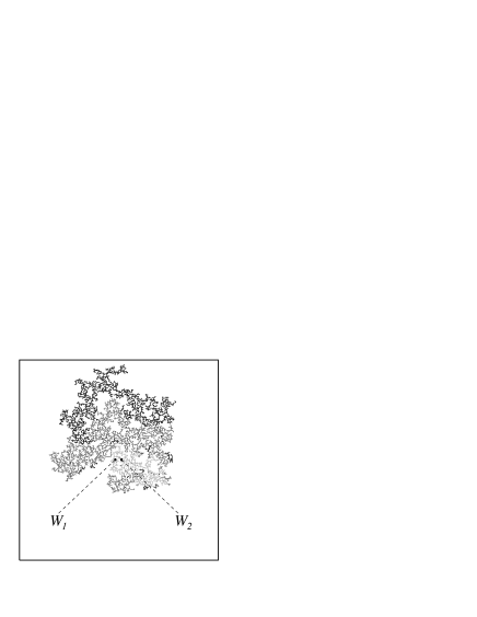
Figure 1: Time evolution of the invasion process between the injection ($W_{1}$) and extraction ($W_{2}$) sites. The steps of invasion are identified in accordance with the number of iterations (time) executed during the simulation process. The colors indicate in which stage of the process the propagation front reached a given site. The light gray sites correspond to the range $1\leqslant t\leqslant 1000$, the dark gray sites to $1000<t\leqslant 5000$, and the black ones correspond to $t>5000$. The pressure value at the extraction well is $p_{e}=0$.

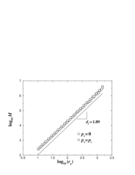
Figure 2: Log-log plot of the radius of gyration for $L=8192$ and $r=4$. The circles correspond to $p_{e}=0$ and the squares to $p_{e}=p_{c}$. These results have been produced with $10000$ realizations of NTIP clusters that do not touch the border of the lattice. The straight line (shifted downwards for better visualization) is the least-square fit to the data and the slope gives the fractal dimension $d_{f}=1.89\pm 0.01$ .

III Results and Discussion

In Fig. 1, we illustrate some stages of the invasion process taking place in a lattice of size $L=256$ and distance between sites $r=16$ . The shades of gray indicate in which interval of time of the process a given site has been invaded. As can be seen from this typical realization of the model, the cluster resulting from the invasion process represents only a small fraction of the network.

In what follows, we show how sensitive is the statistics of the mass of the invaded clusters to the pressure value $p_{e}$ imposed at the extraction site $W_{2}$. Since the invasion finishes as soon as the extraction well is reached, we can interpret that the local pressure $p_{e}$ corresponds to a special criteria to stop the NTIP growth process, without any interference in the microscopic rules of the model. This suggests that the invaded clusters obtained for distinct values of $p_{e}$ should still be in the same universality class observed for invasion percolation between two borders of a lattice. A direct evidence for this fact can be obtained through the calculation of the fractal dimension of the invaded cluster. We show in Fig. 2 the log-log plot of the mass of the invaded cluster against its radius of gyration for $p_{e}=0$ and $p_{e}=p_{c}$. These results have been obtained for, $L=8192$, $r=4$ and $10000$ realizations in which the growth process stopped before the invading cluster reached the border of the lattice. The best linear fit to both data sets gives approximately the same value for the fractal dimension $d_{f}=1.89\pm 0.01$. This value is consistent with the value reported for the standard invasion percolation process, $d_{f}\approx 1.89$ Feder_88 ; Stauffer_94 ; Schwarzer_99 ; Knackstedt_02 . Our results therefore support the assumption that NTIP and SP are in the same universality class Stauffer_94 .

Figure 3: Graph in log-log scale of the mass distribution of invaded clusters $P(M)$ for the case in which the pressure at the extraction site is $p_{e}=0$, and a network size $L=512$. Each curve correspond to a different value for the distance between the wells, namely $r=4$ (plus), $8$ (X) and $16$ (stars). These distributions have been rescaled by its corresponding value $M_{0}$ at the position of the bump. The straight line is the least-square fit to the data in the scaling region with the slope  $-1.39\pm 0.03$. For better visualization the straight line has been slightly shifted upwards, i.e., the ordinate values have been multiplied by an arbitrary constant factor. The corresponding unscaled distributions are shown in inset.

In Fig. 3 we show the log-log plot of the distribution $P(M)$ of invaded masses for the case $p_{e}=0$, and different values of the “well” distance $r$. Clearly, all distributions displays power-law behavior $P(M)\sim M^{-\alpha}$ for intermediate mass values. In addition, a lower cutoff of order $r^{d_{f}}$ is always present, corresponding to the minimum cluster size. The upper cutoff of order $L^{2}$, on its turn, refers to the situation in which almost all sites of the lattice are invaded before the invasion front reaches the extraction site. The effect of $r$ on the distribution is to simply modify the range of the scaling region. The solid line in Fig. 3 corresponds to the best linear fit for the data corresponding to $r=4$ in the scaling region, with the exponent $\alpha=1.39\pm 0.03$. These curves also present a “bump” in the region of large values of mass. For comparison, when we rescale the distributions by their corresponding value at the maximum of this bump $M_{0}$, a collapse in the scaling region can also be observed.

Figure 4: Log-log plot of $P(M)$ for the case $L=256$ and different values for the distance between the wells, $r=4$ (plus), $r=8$ (X), and $r=16$ (star). The pressure at the extraction site is equal to $p_{e}=p_{c}\simeq 0.5927$. The solid line indicates the linear regression (for $r=4$) with the exponent $\alpha=1.00\pm 0.03$. For better visualization, it has been slightly shifted upwards.

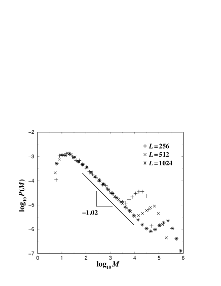
Figure 5: Log-log plot of $P(M)$ for the case $r=4$ and different lattice sizes, $L=256$ (plus), 512 (X), and 1024 (star). The pressure at the extraction site is equal to $p_{e}=p_{c}\simeq 0.5927$. The solid line indicates the linear regression (for $L=1024$) with the exponent $\alpha=1.02\pm 0.03$.

In Fig. 4 we show the distributions of mass $P(M)$ for the case in which the pressure at the site $W_{2}$ is arbitrarily set to $p_{e}=p_{c}\simeq 0.5927$, where $p_{c}$ corresponds to the site percolation threshold of the square network Stauffer_94 . Again, the smaller the distance between the sites, larger is the range over which the power-law behavior holds. In addition, the distributions present the same lower cutoff of order $r^{d_{f}}$ and the upper cutoff of order $L^{2}$, where a bump can also be observed in the region of large values of mass Barth_99 ; Araujo_03 . We show in Fig. 5 the effect of the system size on the distributions of mass for the case $r=4$ and $p_{e}=p_{c}$. The results shown in Figs. 4 and 5 are also consistent with the existence of a power-law regime for intermediate values of mass, $P(M)\sim M^{-\alpha}$, but with an exponent $\alpha=1.02\pm 0.03$. The less negative exponent in the power-law distribution for the cases $p_{e}=p_{c}$ when compared to $p_{e}<p_{c}$ means that, in the later case, larger clusters appear more frequently.

As already mentioned, just before the extraction site is invaded, all sites belonging to the invasion front have their pressure values larger than $p_{e}$. Therefore, in the case where $p_{e}=p_{c}$, the invaded cluster is similar to a cluster generated using the standard percolation (SP) model at the critical point. In the SP model the distribution of cluster sizes follows a power-law, $P(S)\sim S^{-\tau}$, where the exponent $\tau\approx 2.055$ is known as Fisher exponent Stauffer_94 . Assuming that the IP and SP models are compatible, note that, in our model the invaded cluster would be the same if any of its sites were chosen as the injection point. As a consequence, the probability of finding an invaded cluster of size $M$ is the product of two factors, namely, the probability with which such cluster appears in a percolation lattice at the critical point, and the size of the cluster. Thus, we should expect $\alpha=\tau-1\approx 1.055$, a value that is in good agreement with our numerical results.

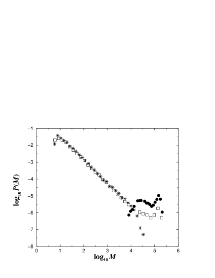
Figure 6: Log-log plot of the distribution $P(M)$ for $p_{e}=0$ and $L=512$. The squares include all clusters, the stars only the clusters that do not touch any of the edges, and the full circles only those that touch the edges of the lattice substrate. All distributions have been normalized by their integrals.

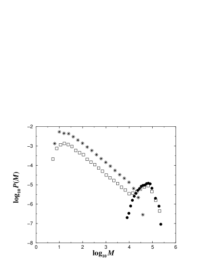
Figure 7: Log-log plot of the distribution $P(M)$ of the invaded cluster $p_{e}=p_{c}$ and $L=512$. The squares include all clusters, the stars only the clusters that do not touch any of the edges, and the full circles only those that touch the edges of the network. All distributions have been normalized by their integrals.

The bumps present in the distributions shown in Figs. 3 and 4 are due to aggregates that grow long enough to reach the border of the lattice before reaching the extraction well. This is made clear when we distinguish these clusters in our simulation data from those that stop before reaching the borders. The distributions shown in Fig. 6 and Fig. 7 reveal that the bumps are mainly originated by the cluster masses subjected to size limitations (full circles), i.e., those clusters that touch the lattice borders. Note that, even after touching the border, the cluster continues to grow until the extraction well is invaded. Thus, those clusters that contribute to the bump in the region of large $M$ have a fractal dimension $d_{f}=2$ and therefore do not possess the critical properties observed in percolation clusters. The statistics of these larger clusters can be investigated if we compute the fraction $\chi$ of invaded clusters that do not touch the edges of the simulation box for different values of the pressure $p_{e}$. As shown in Fig. 8, for a given value of $L$ and $r$, $\chi$ remains approximately constant up to a value of $p\approx p_{c}$ where it experiences a sharp decrease and reaches $\chi=0$. For $p_{e}<p_{c}$, the presence of these large clusters is an artifact of the finite size of the lattice and becomes less relevant as the lattice size grows. In the results which follow we will only consider the clusters that do not touch the borders when computing the distributions of mass.

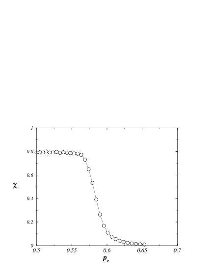
Figure 8: The fraction $\chi$ of invading clusters that do not touch the edges of the network as a function of the pressure value at the extraction site for system size $L=256$ and distance between sites $r=8$.

To better understand how the statistics of the mass distribution changes with the value of the pressure at the extraction site, we perform simulations with different values of $p_{e}=0.0,~{}0.2,~{}0.4,~{}0.55,~{}p_{c}~{}(\simeq 0.5927)$, and $0.6$. From the results presented in Fig. 9, we observe that the distribution $P(M)$ remains practically unchanged (see the inset) with a scaling regime at intermediate values of $M$ that persists at least up to $p_{e}=0.4$. For $p_{e}$ values larger than this, the distribution $P(M)$ changes gradually (see the curve for $p_{e}=0.55$) until another power-law is effectively established at $p_{e}=p_{c}$. For $p_{e}>p_{c}$, most of the generated clusters are subjected to border effects and the scaling behavior is again suppressed.

The behavior of the distributions as $p_{e}$ approaches $p_{c}$ is shown in Fig. 10. For large values of $M$, all curves converge to the same behavior, which coincides with the power-law form obtained for the case $p_{e}=0$. For small values of $M$, the curves display a power-law decay with an exponent that depends on the value of $p_{e}$, but approaches the value $\alpha=1.055$, expected in the limit $p_{e}=p_{c}$. One can understand this behavior by making a parallel with the way in which the standard percolation model approaches the critical point. As $p\to p_{c}$ in SP, the characteristic length of the clusters $\xi$ diverges as $(p_{c}-p)^{-\nu}$, with $\nu=4/3$. Thus, we should observe the critical behavior for values of $M$ bellow the characteristic mass of a cluster obtained with $p=p_{e}$, and the off-critical behavior for values of $M$ above this characteristic mass. It means that the onset of the crossover between the two behaviors should scale as $(p_{c}-p_{e})^{-\gamma}$, with $\gamma=\nu d_{f}$. Assuming that our invasion process is consistent with SP, we expect $\gamma\approx 2.52$. This ansatz is supported by the scaled curves shown in the inset of Fig. 10. As can be seen, for $p_{e}\ll p_{c}$, the crossover moves to values of mass smaller than the cutoff region in $r^{d_{f}}$, and only the off-critical regime is present. On the other hand, for $p_{e}>p_{c}$, most of the generated clusters reach the border of the lattice, leaving the critical regime, and the scaling behavior is again suppressed.

It is possible to understand why we obtain distinct distributions in the critical ($p_{e}=p_{c}$) and off-critical ($p_{e}<p_{c}$) regimes by noting that our invasion percolation process can be divided in the following two sequential phases. In the first phase, the invaded cluster grows from the injection site and reaches an immediate neighborhood of the extraction site. The second phase includes all additional invading steps up to the point in which the extraction site itself is taken, and the invasion process is then terminated. Thus, we can say that the total invaded mass is the sum of two variables, $M=M_{1}+M_{2}$, where $M_{1}$ and $M_{2}$ are the numbers of invasion steps to accomplish the first and second phases, respectively. Since the masses $M_{1}$ and $M_{2}$ have distinct distributions, namely, $P_{1}(M_{1})$ and $P_{2}(M_{2})$, respectively, the distribution with the longer tail between them, should determine the behavior of the tail of $P(M)$. Note that the distribution $P_{1}(M_{1})$ does not depend on the value of $p_{e}$. On other hand, the number of additional steps to invade the extraction well clearly depends on $p_{e}$ and so does $P_{2}(M_{2})$. In the particular case of $p_{e}=0$, it follows that $M_{2}=1$. We can then write that $P(M)=P_{1}(M-1)\simeq M^{-\alpha}$, which shows that the exponent $\alpha=1.39$ comes from the distribution of steps necessary to complete phase 1. When $p_{e}$ approaches $p_{c}$, the contribution of $M_{2}$ to the distribution $P(M)$ starts to become relevant. In the critical condition $p_{e}=p_{c}$, the tail of this distribution is dominated by the number $M_{2}$ of steps to invade the extraction well. Although we lack information about the complete form of $P_{2}(M_{2})$, we know that the necessary condition to invade the extraction well is that all sites belonging to the perimeter of the invaded cluster have pressures $p>p_{e}$. Following percolation theory Stauffer_94 , when $p_{e}=p_{c}$, this condition leads to a power-law distribution, $P(M)\simeq M^{-\alpha}$, where $\alpha=1.055$. As a consequence, we can deduct that, to be dominant, the tail of $P_{2}(M_{2})$ should behave in the same way.

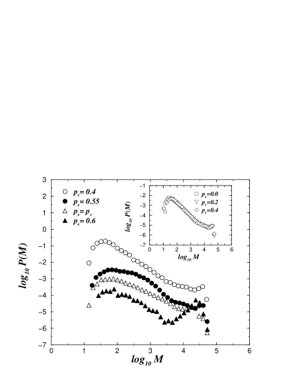
Figure 9: Log-log plot of the mass distribution of the invaded cluster for different values of the pressure at the extraction site. $p_{e}=0.4$ (circles), $p_{e}=0.55$ (full circles), $p_{e}=p_{c}$ (triangles) and $p_{e}=0.6$ (full triangles). The inset shows the mass distribution of invaded cluster for pressure values $p_{e}=0.0$ (circles), $p_{e}=0.2$ (triangles) and $p_{e}=0.4$ (diamond). The system size is $L=256$ and the distance between the injection and extraction sites is $r=8$.

Figure 10: Log-log plot of the mass distribution of the invaded cluster for values of the pressure at the extraction site approaching the critical point $p_{e}=p_{c}$ for systems size $L=8192$. The thin lines are included as guide to eyes and have the slopes expected in the following limiting cases: (i) $-1.05$ for the critical case $p_{e}=p_{c}$ and (ii) $-1.39$ observed in $p_{e}=0$. In the inset, the curves are rescaled by the characteristic mass $\xi^{d_{f}}$, where $\xi$ is the correlation coefficient which scales with the pressure at the extraction well as $\xi\sim(p_{c}-p_{e})^{-\nu}$. The exponents $d_{f}$ and $\nu$ are assumed to be the same as in the the standard percolation model, namely, $d_{f}=1.89$ and $\nu=4/3$.

The invasion percolation is broadly recognized as the most convincing model for a natural phenomenon that displays self-organized critical (SOC) behavior P_Back_88 . Indeed, this characteristic is manifested, for example, in the distribution of the random numbers $P(p)$ corresponding to those sites that have been occupied during the invasion process. Accordingly, the fact that $P(p)$ displays a sharp cut-off on the right side at the critical percolation point $p_{c}$ represents a sound signature of the SOC behavior, which dictates the dynamics of the displacement process. In Fig. 11 we plot the distribution $P(p)$ computed from $1000$ realizations of size $L=512$ and distance $r=4$, and for values of $p_{e}=0,0.61,0.63$ and $0.65$ as well as for $p_{e}=p_{c}$. For $p_{e}=0$ and $p_{e}=p_{c}$, after the completion of the invasion process, both distributions display a clear cutoff at $p\approx p_{c}$, in agreement with previous simulations of the standard invasion percolation model Zara_99 ; Araujo_04 . The inset in Fig. 11 shows that the transition is clearly sharper for $p_{e}=p_{c}$ than for $p_{e}=0$. In the cases in which $p_{e}>p_{c}$, we observe that the cutoff of the distribution $P(p)$ shifts rightwards to $p=p_{e}$. Since we are only interested in those clusters that do not touch the borders, for $p_{e}>p_{c}$, a very large number of trials of the invasion process is necessary to generate the number of realizations required to produce good statistics (see Fig. 8). Once more, if we argue that $p_{e}$ can be interpreted as a stopping criteria for the invasion process, the non-invaded sites that are neighbors of the perimeter sites of clusters generated under such constraint should all have local probabilities that obey the inequality $p>p_{e}$. As a consequence, for $p_{e}>p_{c}$, the invaded clusters are limited by a “high energy” border of non-invaded sites.

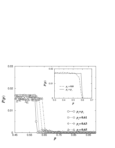
Figure 11: The probability distribution $P(p)$ of invaded sites for different values of the pressure in the extraction site, $p_{e}=p_{c}$ (circles), $0.61$ (squares) and $0.63$ (diamonds) and $0.65$ (triangles) for $L=512$ and $r=4$. The inset shows the probability distribution $P(p)$ for $p_{e}=0.0$ (dotted line) and $p_{c}$ (solid line).

IV Conclusions

In summary, we investigate here the statistics of the mass of the invasion percolation clusters generated between two sites separated by a distance $r$ in a two-dimensional network, and for different values of the local probability at the extraction site, $p_{e}$. The results of our simulations indicate that the distribution of mass of the invaded cluster $P(M)$ is highly sensitive to $p_{e}$. More important, $P(M)$ displays power-law behavior in the following two different conditions: (i) an off-critical regime for sufficiently low values of $p_{e}$, and (ii) a critical regime for $p_{e}=p_{c}$. Interestingly, even though the scaling exponents calculated in both cases are substantially different, namely $\alpha=1.39\pm 0.03$ and $1.02\pm 0.03$ for cases (i) and (ii), respectively, our results for the fractal dimension of the invaded clusters show that they should belong to the same universality class. For $p_{e}$ approaching $p_{c}$, we found that the distribution displays a crossover from the critical to the off-critical regime and that the onset of the crossover scales as $\xi^{d_{f}}$, where $\xi$ is the correlation length, $\xi\sim(p_{c}-p_{e})^{-\nu}$. Finally, we have shown that the SOC behavior of the invasion percolation process is rather robust, even in the situation in which $p_{e}>p_{c}$. In this case, although rarely found, those clusters whose growth has not been affected by the borders of the NTIP system (named here “critical clusters”) present a very peculiar property, namely, that all the non-invaded sites at their perimeters have an anomalously high local probability.

V Acknowledgments

We acknowledge CNPq (CT-PETRO/CNPq), CAPES, FINEP and FUNCAP for financial support.

References

- (1) J. Bear, Dynamics of Fluids in Porous Materials (Elsevier, New York, 1972).
- (2) F. A. Dullien, Porous Media - Fluid Transport and Pore Structure (Academic, New York, 1979).
- (3) J. Feder, Fractals (Plenum Press, New York, 1988).
- (4) D. Wilkinson, J. F. Willemsen, J. Phys. A 16, 3365 (1983).
- (5) D. Stauffer and A. Aharony, Introduction to Percolation Theory (Taylor Francis, Philadelphia, 1994).
- (6) R. Chandler, et al., J. Fluid Mech.119, 249 (1982).
- (7) Fractals and Disordered Systems 2nd ed., edited by A. Bunde and S. Havlin (Springer-Verlag, New York, 1996).
- (8) M. Sahimi, Flow and Transport in Porous Media and Fractured Rock (VCH, Boston, 1995) and the extensive references therein.
- (9) M. Murat and A. Aharony, Phys. Rev. Lett. 57, 1875 (1986).
- (10) J. P. Tian and K. L. Yao, Phys. Lett. A 251, 259 (1999)
- (11) Y. Lee, J. S. Andrade, Jr., S. V. Buldyrev, N. V. Dokholyan, S. Havlin, P. R. King, G. Paul, and H. E. Stanley, Phys. Rev. E. 60 , 3425 (1999).
- (12) B. Clark , and R. Kleinberg, Physics Today 55, 48-53 (2002).
- (13) S. Roux, E. Guyon, J. Phys. A 22, 3693 (1989).
- (14) Mark A. Knackstedt, Muhammad Sahimi, and Adrian P. Sheppard Phys. Rev. E. 65, 035101 (2002).
- (15) M. Barthélémy, S. V. Buldyrev, S. Havlin, and H. E. Stanley, Phys. Rev. E. bf 60, R1123 (1999)
- (16) A. D. Araújo, A. A. Moreira, R. N. Costa, J. S. Andrade Jr., Phys. Rev. E. 67, 027102 (2003).
- (17) S. Schwarzer, S. Havlin and A. Bunde, Phys. Rev. E 59, 3662 (1999).
- (18) M. A. Knackstedt, M. Sahimi and A. P. Sheppard, Phys. Rev. E 65, 035101(R) (2002).
- (19) P. Bak, C. Tang and K. Wiesenfeld Phys. Rev. A 38, 364 (1988).
- (20) R. A. Zara and R. N. Onody, Int. Mod. Phys. C 10, 227 (1999)
- (21) A. D. Araújo, J. S. Andrade Jr. and H. J. Herrmann Phys. Rev. E 70, 066150 (2004).