Nonequilibrium Transport in Quantum Impurity Models
(Bethe-Ansatz for open systems)

Abstract

We develop an exact non-perturbative framework to compute steady-state properties of quantum-impurities subject to a finite bias. We show that the steady-state physics of these systems is captured by nonequilibrium scattering eigenstates which satisfy an appropriate Lippman-Schwinger equation. Introducing a generalization of the equilibrium Bethe-Ansatz - the Nonequilibrium Bethe-Ansatz (NEBA), we explicitly construct the scattering eigenstates for the Interacting Resonance Level model and derive exact, nonperturbative results for the steady-state properties of the system.

The recent spectacular progress in nanotechnology has made it possible to study quantum impurities out-of-equilibrium GG . The impurity is typically realized experimentally as a quantum dot, a tiny island of electron liquid attached via tunnel junctions to two leads (baths or reservoirs) held at different chemical potentials. As a result of the potential difference, an electric current flows from one lead to another across the quantum impurity. The description of such an out-of-equilibrium situation in a strongly correlated system is a long standing problem and has not been given even in the simplest case of when the system is in a steady state.

In a steady state the system properties do not change with time even when out of equilibrium. Such a state is reached only under special conditions: each lead needs to be a good thermal bath and infinite in size (equivalently, the bath level spacing tends to zero.) It then follows that particles transferred from one lead to another dissipate their extra energy in the lead and equilibrate doyon .

There are two equivalent ways, time-dependent and time-independent, to describe the establishment of a steady state in the system. In the time dependent picture the quantum impurity is coupled to the two baths in the far past, $t_{0}$, and is allowed to evolve adiabatically under the conditions described above. After a sufficiently long time, at $t=0$ say, a steady state is reached. Two elements are required to fully determine the system: a hamiltonian to describe the time evolution and an initial condition, $\rho_{0}$, describing the system in the far past. The hamiltonian is chosen to be of the form, $H(t)=H_{0}+e^{\eta t}H_{1}$, where $H_{0}$ describes the two free leads (thermal baths), $H_{1}$ is the interaction term between the leads and the quantum impurity, and $\eta$ an infinitesimal parameter, small enough to ensure adiabaticity yet large compared to the level spacing in the leads. The initial condition is typically given by,

$$\rho_{0}=\frac{e^{-\beta(H_{0}-\sum_{i}\mu_{i}N_{i})}}{Tre^{-\beta(H_{0}-\sum_{i}\mu_{i}N_{i})}}$$ (1)

with $\mu_{i}$ and $N_{i}$ the chemical potential and number operator for particles in lead $i$. Subsequently, at times $t\geq t_{0}$, the system is described by a density matrix $\rho(t)=T\{e^{i\int_{t_{0}}^{t}\,dt^{\prime}H(t^{\prime})}\}\rho_{0}T\{e^{-i\int_{t_{0}}^{t}\,dt^{\prime}H(t^{\prime})}\}$, and the properties of the system are calculated in the usual manner, $\langle\hat{O}(t)\rangle=Tr\{\rho(t)\hat{O}\}$. The establishment of a steady state follows, in this language, from the existence of the limit $t_{0}\to-\infty$ with the expectation value becoming time-independent, $\langle\hat{O}\rangle=Tr\{\rho_{s}\hat{O}\}$ where $\rho_{s}=\rho(0)$.

At $T=0$ the description simplifies. The initial condition is typically given by a particular eigenstate of $H_{0}$, $|\Phi\rangle_{baths}$, describing the baths, each with its own chemical potential $\mu_{i}$. The steady state is then obtained by evolving the initial state in time, $|\Psi\rangle_{s}=T\{e^{i\int_{-\infty}^{t}\,dt^{\prime}H(t^{\prime})}\}|\Phi\rangle_{baths}$. The expectation values in the steady state are computed from,

$$\langle\hat{O}\rangle=\frac{\langle\Psi|\hat{O}|\Psi\rangle_{s}}{\langle\Psi|\Psi\rangle_{s}}$$ (2)

An equivalent way to describe a non-equilibrium steady-state is by means of a time-independent scattering formalism. The state $|\Psi\rangle_{s}$ is obtained as an eigenstate of the full hamiltonian $H=H_{0}+H_{1}$, satisfying the Lippman-Schwinger equation,

$$|\Psi\rangle_{s}=|\Phi\rangle_{baths}+\frac{1}{E-H_{0}\pm i\eta}H_{1}|\Psi\rangle_{s}$$ (3)

with $|\Phi\rangle_{baths}$ - the incoming state. The scattering eigenstate $|\Psi\rangle_{s}$ can be viewed as consisting of incoming particles (the two free Fermi-seas) described by $|\Phi\rangle_{baths}$ and reflected outgoing particles given by the second term in the above equation. Once again two elements are required to fully determine the system: a hamiltonian and a boundary condition, $|\Phi\rangle_{baths}$, which describes the scattering state far from the impurity. Note that previously, in the time-dependent picture $|\Phi\rangle_{baths}$ played the role of an initial condition rather than a boundary condition. The finite temperature description in this formalism is obtained by summing over scattering states weighted according to the Boltzman weights of the corresponding incoming states.

The construction of such eigenstates is a formidable task in general. We shall show, however, that it can be carried out for a class of integrable impurity models that includes the Interacting Resonance Level Model (IRLM) and the Kondo Model. The Bethe Ansatz solution of these integrable models in equilibrium has led to a full understanding of their thermodynamic properties. It is based on solving the hamiltonian of a closed system, typically with periodic boundary conditions. We shall present in this letter a significant generalization of the Bethe Ansatz approach to open systems with boundary conditions imposed by the leads. This approach, the Non-equilibrium Bethe-Ansatz (NEBA), allows us to construct the fully interacting multi-particle scattering eigenestates and compute non-equilibrium transport properties, extending Landauer’s original approach land . We remark here that our approach differs significantly from the recent interesting work by Konik et al. konik who also used integrability to compute transport. In contrast to their work we model the leads as free Fermi seas rather than coupling the chemical potentials to dressed excitations.

We focus on the IRLM at $T=0$ and defer treatment of other models to later publications. The IRLM, $H_{\rm{IRL}}=\sum_{i=1,2,\vec{k}}\epsilon_{k}\psi_{i\vec{k}}^{\dagger}\psi_{i\vec{k}}+\epsilon_{d}d^{\dagger}d+\;\frac{t}{\sqrt{2}}\sum_{i=1,2,\vec{k}}(\psi_{\vec{k}}^{\dagger}d+h.c.)+\;2U\sum_{i=1,2,\vec{k},\vec{k^{\prime}}}\psi_{i\vec{k}}^{\dagger}\psi_{i\vec{k^{\prime}}}d^{\dagger}d$, describes a resonant level, $\epsilon_{d}d^{\dagger}d$, coupled to two baths of spinless electrons via tunneling junctions with strength $t$. There is also a Coulomb interaction $U$ between the the level and the baths. The model is closely related to the anisotropic Kondo model WF , with the charge states $n_{d}=0,1$ playing the role of spin states, and $\epsilon_{d}$ playing the role of a local magnetic field.

Performing some standard manipulations for impurity models: expanding in angular modes around the impurity, keeping only the s-modes, unfolding the model, and linearizing around the two Fermi points we have,

$$H_{\rm{IRL}} = -i\sum_{i=1,2}\int\,dx\,\psi_{i}^{\dagger}(x)\partial\psi_{i}(x)+\epsilon_{d}d^{\dagger}d$$

$$+ \frac{t}{\sqrt{2}}(\sum_{i=1,2}\psi_{i}^{\dagger}(0)d+h.c.)+2U\sum_{i=1,2}\psi_{i}^{\dagger}(0)\psi_{i}(0)d^{\dagger}d.$$

The model thus obtained is a renormalizable field theory which requires introduction of a cut-off procedure to render it finite. The values of the bare parameters $U,\epsilon_{d},t$ will be renormalized as the cut-off is removed to yield a physical theory. The renormalized theory captures the universal physics - where voltages and temperatures are small compared to the cut-off (bandwidth $D$). The chemical potentials for the leads are not included in the Hamiltonian. Instead, they enter as nonequilibrium boundary conditions specifying the scattering-state far from the impurity.

We wish to calculate the expectation values in the steady state of the dot occupation, $\hat{n}_{d}=d^{\dagger}d$, and the current operator, $\hat{I}=\frac{i}{2}\sum_{j=1,2}(-1)^{j}t/\sqrt{2}(\psi_{j}^{\dagger}(0)d-h.c)$, the latter deduced from $\hat{I}=\frac{1}{2}[(N_{1}-N_{2}),H]$.

To construct the scattering states we shall use a new Bethe-Ansatz technique which, unlike the traditional approach based on closed systems and periodic boundary conditions, allows the determination of a state by boundary conditions imposed asymptotically. We shall build the many body scattering state using single particle scattering states that incorporate the boundary conditions. It is convenient to introduce the symmetric/anti-symmetric basis defined by $\psi_{e/o}(x)=\frac{1}{\sqrt{2}}(\psi_{1}(x)\pm\psi_{2}(x))$, in terms of which the hamiltonian separates into even and odd parts, $H_{e}=-i\int\,dx\,\psi_{e}^{\dagger}(x)\partial\psi_{e}(x)+U\psi_{e}^{\dagger}(0)\psi_{e}^{\dagger}(0)d^{\dagger}d+t(\psi_{e}^{\dagger}(0)d+h.c.)+\epsilon_{d}d^{\dagger}d$, and $H_{o}=-i\int\,dx\,\psi_{o}^{\dagger}(x)\partial\psi_{o}(x)+U\psi_{o}^{\dagger}(0)\psi_{o}^{\dagger}(0)d^{\dagger}d.$ The boundary conditions, however, are imposed in the physical basis, $\psi_{1/2}$, requiring appropriate combinations of both the even and odd sectors. Both hamiltonians conserve the number of particles: $H_{e}$ commutes with $\bar{N}_{e}=N_{e}+N_{d}$ and $H_{o}$ with $N_{o}$. The construction proceeds by considering the $N$-particle sacttering solutions, $N=1,2,\cdots$ It is important to note that in doing so we have imposed cut-offs on the theory. Only upon taking the limit $N,L\to\infty$ is the field theory regained and the results become universal.

The single-particle eigenstates of the model take the form,

$$\int dx\,[A(g_{p}(x)\psi_{e}^{\dagger}(x)+e_{p}d^{\dagger})+Bh_{p}(x)\psi_{o}^{\dagger}(x)]|0\rangle$$ (5)

with $|0\rangle$ the empty vacuum and $A$ and $B$ arbitrary constants chosen to satisfy the nonequilibrium boundary conditions. We are interested in two solutions, labeled $\pm$, to the Schrodinger equation for these eigenstates,

$$g_{p}(x) = \frac{2e^{ipx}}{1+e^{i\delta_{p}}}\left[\theta(-x)+e^{i\delta_{p}}\theta(x)\right],\quad(g_{p}(0)=1)$$

$$h_{p}^{\pm}(x) = \frac{2e^{ipx}}{1+e^{i\delta_{p}}}\qquad\qquad\qquad\qquad\quad\qquad\;\;x\neq 0$$

$$h_{p}^{\pm}(0) = \pm\frac{(p-\epsilon_{d})e_{p}e^{ipx}}{t}=\pm g_{p}(0)e^{ipx}\qquad x=0$$ (6)

with $e_{p}=tg_{p}(0)/(p-\epsilon_{d})$ and $\delta_{p}=2\arctan\left[\frac{t^{2}}{2(p-\epsilon_{d})}\right]$. In writing these states, we have chosen the regularization scheme: $\theta(\pm x)\delta(\pm x)=\frac{1}{2}\delta$. Note, that we take $h_{p}(x)$ to be discontinuous at zero. This unorthodox choice of solution is allowed by the linear derivative. Theories with linear derivatives – as realized by Dirac long ago – are implicitly many-body theories. To calculate physical observables, one must first fill the Fermi-sea from a lower cut-off $D$ to the Fermi energy. Since the universal many body physics is only sensitive to the amplitude of $h_{p}(x)$ before and after the impurity, renormalizability implies that physical observables are insensitive to the choice of discontinuities in $h_{p}(x)$ AFL .

We construct two kinds of single-particle scattering states, namely those with incoming particles from lead-1, $|1p\rangle$, and those with incoming particles from lead-2, $|2p\rangle$, with $p$ the momentum of the incoming particle. Choosing $A=B$ in eq(5), the amplitude for an incoming particle from lead-2 vanishes and we get,

$$|1p\rangle = \int dx\,e^{ipx}\left[\frac{2}{1+e^{i\delta_{p}}}\left([2\theta(-x)+(e^{i\delta_{p}}+1)\theta(x)]\psi_{1}^{\dagger}\right.\right.$$

$$+ \left.\left.[(e^{i\delta_{p}}-1)\theta(x)]\psi_{2}^{\dagger}\right)+\sqrt{2}e_{p}d^{\dagger}\delta(x)\right]|0\rangle$$

Conversely, choosing $A=-B$, the amplitude for an incoming particle from lead-1 vanishes and we get the state $|2p\rangle$, given by the above expression with $\psi_{1}^{\dagger}(x)$ and $\psi_{2}^{\dagger}(x)$ interchanged. It is convenient to introduce the operators, $\alpha_{1/2p}^{\dagger}(x)=g_{p}(x)\psi_{e}^{\dagger}(x)\pm h_{p}^{\pm}(x)\psi_{o}^{\dagger}(x)+e_{p}\delta(x)d^{\dagger}$, in terms of which the scattering states are $|1/2p\rangle=\int dxe^{ipx}\alpha_{1/2p}^{\dagger}(x)|0\rangle$. The single particle scattering eigenstates are depicted in FIG. 1.

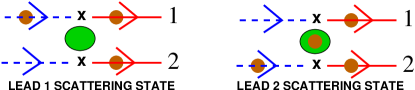
Figure 1: There are two types of single particle scattering states. In type-1 scattering state, an incoming electron in lead 1 is scattered by the impurity and can hop on to either lead 1 or lead 2. Notice there is no amplitude for an electron to initially be in lead 2. In a type-2 scattering state, the role of the two leads is reversed.

The most general two-particle eigenfunction is of the form,

$$\int\int[Ag(x_{1},x_{2})\psi_{e}^{\dagger}(x_{1})\psi_{e}^{\dagger}(x_{2})+Ch(x_{1},x_{2})\psi_{o}^{\dagger}(x_{1})\psi_{o}^{\dagger}(x_{2})$$

$$+\int\int Bj(x_{1},x_{2})\psi_{e}^{\dagger}(x_{1})\psi_{o}^{\dagger}(x_{2})]|0\rangle$$

$$+\int[Ae(x)\psi_{e}^{\dagger}(x)d^{\dagger}+Bf(x)\psi_{0}^{\dagger}(x)d^{\dagger}]|0\rangle$$ (7)

with,

$$2g(x_{1},x_{2}) = g_{p}(x_{1})g_{k}(x_{2})Z(x_{1}-x_{2})-(1\leftrightarrow 2)$$

$$2h(x_{1},x_{2}) = h_{p}(x_{1})h_{k}(x_{2})Z(x_{1}-x_{2})-(1\leftrightarrow 2)$$

$$j^{ab}(x_{1},x_{2}) = g_{p}(x_{1})h_{k}^{a}(x_{2})Z(x_{1}-x_{2})$$ (8)

$$+ (-1)^{ab}g_{k}(x_{1})h_{p}^{b}(x_{2})Z(x_{2}-x_{1})$$

with $a,b=\pm$, $g_{p}(x)$ and $h_{p}^{a/b}(x)$ being the single particle eignefunctions eq(6) and $Z(x_{1}-x_{2})=e^{i\varphi(p,k)\rm{sgn}(x_{1}-x_{2})}$ with $e^{2i\varphi(p,k)}=(i+\frac{U}{2}\frac{p-k}{k+p-2\epsilon_{d}})/(i-\frac{U}{2}\frac{p-k}{k+p-2\epsilon_{d}})$. The constants $A$, $B$, and $C$ are determined by the nonequilibrium boundary conditions. In this solution, we made use of freedom afforded by the linear dispersion to choose the two-particle S-matrix between all electrons to be the same. This allows us to easily generalize the construction to $N$ particle wave functions yielding the fully-interacting scattering state,

$$|\Psi\rangle_{s}=\int dx\Psi(x_{1}\cdots x_{N})\prod_{u=1}^{N_{1}}\alpha_{1p_{u}}^{\dagger}(x_{u})\prod_{v=N_{1}+1}^{N_{1}+N_{2}}\alpha_{2p_{v}}^{\dagger}(x_{v})|0\rangle$$

$$\Psi_{s}(x_{1}\cdots x_{N})=e^{i\sum_{j}p_{j}x_{j}}e^{i\sum_{s<t}\varphi(p_{s},p_{t})sgn(x_{s}-x_{t})}\quad\qquad\quad$$ (9)

Recall that for $|\Psi\rangle_{s}$ to describe a non-equilibrium steady-state the incoming particles in the region $\{x_{j}\}\leq 0$ must be described by $|\Phi\rangle_{baths}$. In the coventional Fock basis $|\Phi\rangle_{baths}$ is given by: $\prod_{u=1}^{N_{1}}e^{i\sum_{u}\bar{p}_{u}x_{u}}\prod_{v=N_{1}+1}^{N_{1}+N_{2}}e^{i\sum_{v}\bar{p}_{v}x_{v}}$, with the Fock momenta $\{\bar{p}_{j}\}$ satisfying: $-D\leq\bar{p}_{u}\leq\mu_{1}$ and $-D\leq\bar{p}_{v}\leq\mu_{2}$. Notice, however, that in $\Psi_{s}(x_{1}\cdots x_{N})$ there is a two particle $S$-matrix, $S=e^{2i\varphi(p,k)}$, between incoming particles in each lead though the particles are free electrons. The presence of this non-trivial S-matrix forces a choice of a different, “Bethe-Ansatz”, basis of eigenstates for the free Fermi seas in the leads, inherited from the interacting model when the coupling to the impurity is turned off natan . In order impose the boundary condition in the Bethe-Ansatz basis, the incoming particles “Bethe-Ansatz” momenta $\{p_{j}\}$ in $|\Psi\rangle_{s}$, thus far undetermined, must be appropriately chosen. This is done below by solving “free-field” Bethe-Ansatz equations.

The steady-state current and dot occupation in the non-equilibrium steady-state is computed from eq(2) with $\hat{O}$ the appropriate operator and $|\psi\rangle$ given by eq(LABEL:U=0scatteringstate). When computing this expectation value, one must take the system size, $L$, to infinity (recall that no steady state can be reached otherwise). In this limit, scattering states of type 1 and 2 are orthogonal and we find,

$$\langle I\rangle_{s}=\sum_{u=1}^{N_{1}}\frac{\Delta^{2}}{(p_{u}-\epsilon_{d})^{2}+\Delta^{2}}-\sum_{v=N_{1}+1}^{N_{1}+N_{2}}\frac{\Delta^{2}}{(p_{v}-\epsilon_{d})^{2}+\Delta^{2}}$$

$$\langle n_{d}\rangle_{s}=\sum_{u=1}^{N_{1}}\frac{\Delta}{(p_{u}-\epsilon_{d})^{2}+\Delta^{2}}+\sum_{v=N_{1}+1}^{N_{1}+N_{2}}\frac{\Delta}{(p_{v}-\epsilon_{d})^{2}+\Delta^{2}}.$$

with $\Delta=t^{2}/2$. In the non-interacting case, $U=0$, imposing the boundary condition in the thermodynamic limit, the sums are replaced by integrals over $\rho_{i}$ - product of the density of states $\nu=1/2\pi$ and the Fermi-Dirac function - that describe the distribution of momenta in each lead, e.g. at $T=0$, $\rho_{i}(p)=\frac{1}{2\pi}\theta(k^{i}_{o}-p)$, with $k^{i}_{o}$ set by $\mu^{i}$. We obtain the standard RL results meir ,

$$\langle I\rangle_{s} = \int\,dp\left[\rho_{1}(p)-\rho_{2}(p)\right]\frac{\Delta^{2}}{(p-\epsilon_{d})^{2}+\Delta^{2}}$$

$$\langle n_{d}\rangle_{s} = \int\,dp\left[\rho_{1}(p)+\rho_{2}(p)\right]\frac{\Delta}{(p-\epsilon_{d})^{2}+\Delta^{2}}$$ (10)

In the interacting case, however, $\rho_{i}(p)$ are no longer Fermi-Dirac distributions. As explained above, the presence of the non-trivial $S$-matrix requires the distribution in each lead to be obtained by solving a set a free Bethe-Ansatz equations. For $T=0$, the distributions, $\rho_{i}(p),i=1,2$ satisfy,

$$\rho_{1}(p)=\frac{1}{2\pi}\theta(k^{1}_{o}-p)-\sum_{j=1,2}\int_{-\infty}^{k^{j}_{o}}{\cal K}(p,k)\rho_{j}(k)\;dk$$

$$\rho_{2}(p)=\frac{1}{2\pi}\theta(k^{2}_{o}-p)-\sum_{j=1,2}\int_{-\infty}^{k^{j}_{o}}{\cal K}(p,k)\rho_{j}(k)\;dk$$

with $k^{i}_{o},i=1,2$ upper bounds on the distributions of $k$ set by the chemical potentials $\mu_{i}$ (we choose $k^{1}_{o}>k^{2}_{o}$), ${\cal K}(p,k)=\frac{U}{\pi}(k-\tilde{\epsilon}_{d})/[(p+k-2\tilde{\epsilon}_{d})^{2}+\frac{U^{2}}{4}(p-k)^{2}]$ and $\tilde{\epsilon}_{d}=\epsilon_{d}-U\sum_{i=1,2}\frac{N_{i}}{L}$. The equations need be solved in the presence of a cut-off $D$, $-D\leq k$. For $T>0$ one needs to solve the corresponding finite temperature Thermodynamic Bethe Anatz equations.

In the $U=\infty$ limit, these equations can be solved by a standard, if tedious,Wiener-Hopf method yielding the results $\langle I\rangle_{s}=\frac{\Delta}{2\pi}\left(\frac{T_{k}}{\Delta}\right)\left[\tan^{-1}\frac{\mu_{1}-\epsilon_{d}}{T_{k}}-\tan^{-1}\frac{\mu_{2}-\epsilon_{d}}{T_{k}}\right]$ and $\langle n_{d}\rangle_{s}=\frac{1}{2}+\frac{1}{2\pi}\left(\frac{T_{k}}{\Delta}\right)\left[\tan^{-1}\frac{\mu_{1}-\epsilon_{d}}{T_{k}}+\tan^{-1}\frac{\mu_{2}-\epsilon_{d}}{T_{k}}\right]$ where $T_{k}=D\left(\frac{\Delta}{D}\right)^{\frac{2\pi}{\pi+\zeta}}$ with $e^{i\zeta(U)}=\frac{(1-\left[\frac{U}{2}\right]^{2}+2i\frac{U}{2}}{1+\left[\frac{U}{2}\right]^{2}}$. $T_{k}$ is a new low energy scale in the problem, related to the Kondo temperature in the anisotropic Kondo model. It is held fixed as the cut-off and $U$ are sent to infinity.

More generally, these equations must be solved numerically with the bandwidth, $D$, much larger than all parameters in the problem to ensure we are in a universal regime.

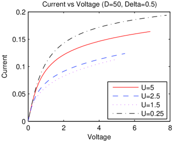
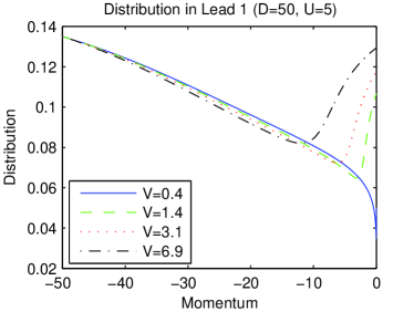
Figure 2: Here we show the current as a function of voltage for various $U$ with $\mu_{1/2}=\tilde{\epsilon_{d}}\pm V/2$ for fixed bandwidth $D$ and $\Delta$. Note,the current is not monotonic in $U$. We also show the distribution in lead 1 as a function of momentum for various voltages where with out loss of generality we take $k_{o}^{1}=0$.

In FIG. 2, we plot our results for the current as a function of voltage for various values of $U$. Notice the current is non-monotonic in U with a duality between small and large $U$. This duality holds for all $\Delta$. We also plot the distribution function in lead 1, $\rho_{1}$, as a function of momentum for various voltages. The strong dependence on momentum and voltage of these distributions is a hallmark of the nonequilibrium physics.

For $\mu_{1}=\mu_{2}$ the system reverts to equilibrium and our construction can be compared with traditional Bethe Ansatz approaches. There is no current in this case, and the dot occupation can be obtained from the impurity energy, given at zero temperature by $E_{imp}=\int\,dp\rho(p)\delta_{p}$ with $\rho(p)$ determined by the TBA equation. Hence, ignoring $\partial_{\epsilon_{d}}\rho(p)$, which is suppressed by $N/L$, we have $\langle n\rangle_{d}=\partial_{\epsilon_{d}}E_{imp}=\int\,dp\rho(p)\partial_{\epsilon_{d}}\delta_{p}$. Since $\partial_{\epsilon_{d}}\delta_{p}=2\Delta/((p-\epsilon_{d})^{2}+\Delta^{2})$, it coincides with eq(10) when $\rho_{1}(p)=\rho_{2}(p)=\rho(p)$.

In conclusion, we have presented an exact solution of a strongly correlated impurity model out of equilibrium. The solution is given in terms of the scatteringing states that characterize the nonequilibrium steady state. The generalization to finite temperature or to more than two leads is straightforward. The latter allows the computation the nonequilibrium density of states eran which is of experimental interest. We believe the framework we introduced is very general and can be applied to most integrable models. Thus far we have constructed current carrying scattering states for the Anderson and Kondo models, though we do not know a general criterion for the framework’s applicability. Neither do we have a classification of the operators whose non-equilibrium expectation values can be calculated.

Acknowledgments: This work was started in collaboration with Y. Gefen during a visit to the Weizmann Institute in Feb. 2001. We thank him for his warm hospitality and generous help. We are grateful to C. Bolech, E. Boulat, O. Parcollet, A. Rosch and especially to B. Doyon and A. Schiller for numerous useful and enlightening discussions. The authors were supported in part by BSF grant 4-21388.

References

• (1) D. Goldhaber-Gordon, Hadas Strickman, D. Mahalu, D. Abusch-Magder, U. Meirav and M. A. Kastner, Nature 391, 156 (1998); D. Goldhaber-Gordon, J. Gores, M. A. Kastner, Hadas Strickman, D. Mahalu and U. Meirav, Phys. Rev. Lett. 81 5225 (1998); S. M. Cronenwett, T. H. Oosterkamp and L. P. Kouwenhoven, Science 281, 540 (1998); J. Schmid, J. Weis, K. Eberl, and K. Von Klitzing, Physica B258, 182 (1998).
• (2) See for example: Benjamin Doyon and Natan Andrei, Universal aspects of non-equilibrium currents in a quantum dot, cond-mat/0506235
• (3) R. M. Konik, H. Saleur, and A. Ludwig, Phys. Rev. B 66, 125304 (2002).
• (4) P. B. Wiegmann and A. M. Finkelstein, Sov. Phys. JETP 48, 102, (1978). For the integrability of the IRLM see: V. M. Filyov and P. B. Wiegmann, Phys. Lett. 76A, 283.
• (5) Discontinuities in Bethe-Ansatz wave functions have appeared before. For a discussion see, N. Andre, K. Furuya and J. H. Lowenstein, Rev. Mod. Phys. 56, p. 331 (1984), section VI.
• (6) N. Andrei, Integrable Models in Condensed Matter Physics, in Series on Modern Condensed Matter Physics - Vol. 6, World Scientific, cond-mat/9408101. J. H. Lowenstein, Les Houches lectures 1982.
• (7) R. Landauer, Phil. Mag. 21 863 (1970).
• (8) A.-P. Jauho, N. S. Wingreen, and Y. Meir Phys. Rev. B 50, 5528 (1994).
• (9) E. Lebanon and A. Schiller, Phys. Rev. B 65, 035308 (2002)