Spectral and polarization effects in deterministically nonperiodic multilayers containing optically anisotropic and gyrotropic materials

Abstract

Influence of material anisotropy and gyrotropy on optical properties of fractal multilayer nanostructures is theoretically investigated. Gyrotropy is found to uniformly rotate the output polarization for bi-isotropic multilayers of arbitrary geometrical structure without any changes in transmission spectra. When introduced in a polarization splitter based on a birefringent fractal multilayer, isotropic gyrotropy is found to resonantly alter output polarizations without shifting of transmission peak frequencies. The design of frequency-selective absorptionless polarizers for polarization-sensitive integrated optics is outlined.

Keywords: Non-periodic deterministic structures, anisotropy, gyrotropy, chiral media, integrated optical polarizers.

1 Introduction

Periodic nanostructured media, also known as photonic crystals (see, e.g., [1, 2] and references therein), have put forth a wide range of possible applications in optical communication, optoelectronics and optical means of data transmission. In addition, photonic crystals have inspired a lot of fundamental research on light-matter interaction, since electromagnetic wave propagation phenomena in strongly inhomogeneous media have been for the first time available for direct theoretical investigation.

Moreover, during the recent decade it was shown that further alteration of topology of inhomogeneous media leads to an even wider choice of optical materials. Within this scope, non-periodic deterministic (NPD) structures have been extensively studied during the recent decade. Namely, quasiperiodic [3, 4, 5] and fractal [6, 7, 8] nanostructures are known to possess distinct optical properties, not present in either periodic or disordered systems. The most interesting among these are spectral self-similarity and critical eigenstates in Fibonacci quasiperiodic lattices [3] and spectral scalability in Cantor fractal multilayers [6], which was shown to directly result from geometrical self-similarity [8].

However, nearly in all the research in this field only optically isotropic constituent materials are considered. On the other hand, there have been recent reports with investigation of anisotropic materials embedded into a periodic structure. For example, it was shown that anisotropy can cause even a one-dimensional (1D) multilayer structure to exhibit negative refraction [9, 10], a phenomenon earlier attributed exclusively to higher-dimensional systems, as well as omnidirectional total transmission [9, 11]. In addition, interesting results have been recently obtained with weakly modulated periodic structures made of anisotropic and gyrotropic materials [12]. Extensive ongoing analytical research of anisotropic and gyrotropic multilayers [13, 14, 15], as well as studies of a simpler case of chiral media in 2D [16] and 3D [17] photonic crystals, is also restricted to periodic systems.

From what has been said, there is a need to “bridge the gap” and combine anisotropy and non-periodicity in the same structure. It is of particular interest to find out how optical anisotropy of constituent materials can affect the spectral properties caused by deterministic non-periodic geometry.

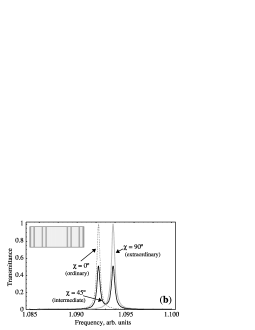
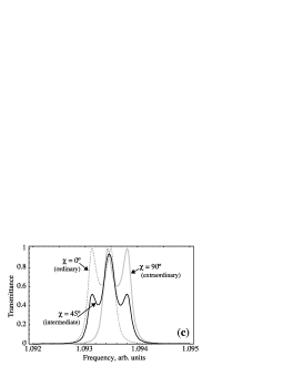
Figure 1: A portion of spectrum of a 27-layer Cantor fractal multilayer structure as a typical spectrum of an NPD structure (a) along with the image of one peak (b) at different orientations of input wave polarization. The peak exhibits polarization-induced splitting [18]. Sometimes, a doublet may split in such a way that matching occurs (c). The inset shows the structure geometry, which can be written as $gagaaagagaaaaaaaaagagaaagag$, $g$ being GaN ($\varepsilon_{o}=5.685$, $\varepsilon_{e}=5.892$) and $a$ being air quarter-wave layers. Frequency is normalized to $\omega_{0}$ defined as $n_{g}d_{g}=n_{a}d_{a}\equiv\lambda_{0}/4=\pi c/2\omega_{0}$ [18].

Our earlier communication [18] showed that for any multilayer structure exhibiting sharp resonance peaks inside a band gap (generally, a characteristic feature of NPD geometry) anisotropy results in polarization-induced peak splitting (figure 1a,b). In this regime, the structure acts as a nanosized absorptionless frequency-selective polarizer, which can in itself find certain applications. Moreover, in the case when a doublet undergoes polarization-induced splitting in such a way that the components are matched (figure 1c), the structure acts as a quarter-wave retarder (QWR) and converts a linearly-polarized beam into circularly-polarized and vice versa. The size of such a retarder is smaller than that of a bulk QWR, and the content of birefringent material is more than 10 times decreased, which suggests enhancement of effective birefringence when anisotropic material in organized in deterministic non-periodic manner.

Of the geometries in question, fractal structures are of special interest because their spectra can provide resonance peaks with controlled multiplicity due to sequential peak splitting [6].

In this paper, we move on to further analyze the optical properties of non-periodic media containing optically anisotropic constituent materials. Along with conventional birefringence, we analyze the effects caused by optical activity (or gyrotropy) [19]. We show numerically as well as analytically that in the case of bi-isotropic multilayers (isotropic optical activity introduced into an initially isotropic medium) gyrotropy does not cause polarization-induced splitting – contrary to what might have been expected. In fact, gyrotropy even does not manifest itself in the spectral characteristics of the multilayer, its sole influence being a geometry-independent polarization plane rotation of the transmitted wave. Furthermore, we show that optical activity can be made use of to modify the polarization sensitivity and the output polarization of a birefringent polarizer described above, meaning both polarization orientation and ellipticity. Possible applications for integrated optics and optical engineering are also outlined.

To account for gyrotropy, we make use of coordinate-free operator formalism for the general case of bi-anisotropic multilayers [20, 21]. It is outlined briefly in Section 2. The simplest case of a multilayer with bi-isotropic layers is analytically and numerically investigated in Section 3. It is shown that gyrotropy can only provide polarization plane rotation completely independent of structure geometry. The combination of isotropic optical activity and uniaxial birefringence is analyzed in Section 4, and it is shown that in this case gyrotropy can be used to control the output polarization of an integrated optical polarizer. Section 5 summarizes the paper.

2 Evolution operator for anisotropic and gyrotropic media

Before proceeding, it is necessary to briefly touch upon the theoretical approaches used. Contrary to the case with isotropic media when common transfer matrix methods with scalar field values would suffice, anisotropic and gyrotropic media cannot be regarded without accounting for polarization effects. Such effects include, for instance, polarization coupling at layer interfaces, so in the general case wave polarization cannot be separated into independent states and full vector calculations have to be performed.

Among the methods for such calculation, we have used the coordinate-free operator method (also known as Fedorov’s covariant approach [19, 20, 22]), developed for stratified systems in [21]. In this method most equations remain in compact form containing only the inherent parameters of the structure. This provides flexibility and facilitates analytical investigation of the equations used.

To account for arbitrary anisotropy and gyrotropy, the following form of material equations is used [21]:

$$\mathbf{D}=\varepsilon\mathbf{E}+i\alpha\mathbf{H},\quad\mathbf{B}=\mu\mathbf{H}+i\beta\mathbf{E}.$$ (1)

Here $\varepsilon$ and $\mu$ are dielectric permittivity and magnetic permeability, respectively. In optically anisotropic media, $\varepsilon$ is a tensor rather than just a scalar coefficient. In materials possessing magnetic anisotropy, $\mu$ can also be a tensor. The quantities $\alpha$ and $\beta$, also tensorial in the general case, are called gyration pseudotensors and are responsible for the material’s optical activity. In non-absorbing media they must satisfy the relation $\beta=-\alpha^{\dagger}$ (Hermitian conjugation). The material equations (1) can in theory encompass all possible cases of anisotropy and gyrotropy [19].

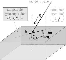
Figure 2: Illustration of an ambient medium / layer interface: on the definition of a natural basis in (2).

Considering a plane wave incident from isotropic ambient medium with refractive index $n_{0}$ onto a slab of a material with parameters given in (1), one can define the wave by its vector of refraction $\mathbf{m}=n_{0}\mathbf{n}$, $\mathbf{n}$ being the vector of wave normal (figure 2). Analogously, the boundary can be characterized by the unit normal vector $\mathbf{q}$ and the corresponding projection operator

$$I=\mathbf{1}-\mathbf{q}\otimes\mathbf{q}=-(\mathbf{q}^{\times})^{2},$$

which projects any vector into the interface plane. Here the notation $\mathbf{u}\otimes\mathbf{v}$ denotes an outer product (also termed the dyad [21]) between two vectors $\mathbf{u}$ and $\mathbf{v}$, which is a tensor with elements in the form $(\mathbf{u}\otimes\mathbf{v})_{ij}=u_{i}v_{j}$, and the symbol $\mathbf{q}^{\times}$ stands for an antisymmetric tensor defined via vector cross product as $(\mathbf{q}^{\times})\mathbf{u}=\mathbf{q}\times\mathbf{u}$, or via fully antisymmetric Levi-Civita’s pseudotensor $\mathcal{E}_{ijk}$ as $\left(\mathbf{q}^{\times}\right)_{jk}=\mathcal{E}_{ijk}\mathbf{q}_{i}$.

Using these elements as a reference, one can further introduce the vectors

$$\mathbf{b}=I\mathbf{m},\quad\mathbf{a}=\mathbf{b}^{\times}\mathbf{q}.$$ (2)

The three vectors $(\mathbf{a}_{0}\equiv\mathbf{a}/|\mathbf{a}|,\mathbf{b}_{0}\equiv\mathbf{b/}|\mathbf{b}|,\mathbf{q})$ are of unit length and mutually orthogonal. Thus they form a basis in space (see figure 2). Note that at normal incidence $\mathbf{a}=\mathbf{b}=0$, which results from axial symmetry of such a system. In this particular case only one of the basis vectors can be introduced naturally, while $\mathbf{a}_{0}$ and $\mathbf{b}_{0}$ are subject to arbitrary choosing.

It was shown earlier [21] that Maxwell’s equations with (1) can be transformed into an operator differential equation

$$\begin{array}[]{l}\frac{d}{dx}\mathbb{W}(x)=ik\mathbb{MW}(x),\\ \\ \mathbb{W}(x)=\left[\begin{array}[]{c}I\mathbf{H}(x)\\ \mathbf{q}^{\times}\mathbf{E}(x)\end{array}\right],\quad\mathbb{M}=\left[\begin{array}[]{cc}A&B\\ C&D\end{array}\right].\end{array}$$ (3)

Here $\mathbb{M}$ is a characteristic block matrix (or characteristic operator) whose elements are operators dependent on the material parameters of the slab. It can be represented by a $6\times 6$ matrix. However, the block matrix notation allows to discriminate between real space [where we have introduced the vectors (2)] and “artificial” $2\times 2$ space related to block vectors $\mathbb{W}$, introduced because electric and magnetic field evolution has to be accounted for simultaneously. To differentiate from real-space vectors and operators, block vectors and matrices are denoted by light capital symbols.

So the components of the characteristic matrix in (3) are operators acting in real space. For their full form one can refer to [21]. Throughout this paper, normal incidence will be considered both in analytical and in numerical investigations. This makes certain sense from the experimental point of view because otherwise gyrotropy is known to be completely shadowed by common birefringence. In this case,

$$\begin{array}[]{l}A=i\mathbf{q}^{\times}\alpha I+[\mathbf{q}^{\times}\varepsilon\mathbf{q}\otimes\mathbf{v}_{3}+i\mathbf{q}^{\times}\alpha\mathbf{q}\otimes\mathbf{v}_{1}],\\ B=-\mathbf{q}^{\times}\varepsilon\mathbf{q}^{\times}+[\mathbf{q}^{\times}\varepsilon\mathbf{q}\otimes(\mathbf{q}^{\times}\mathbf{v}_{4})+i\mathbf{q}^{\times}\alpha\mathbf{q}\otimes(\mathbf{q}^{\times}\mathbf{v}_{2})],\\ C=I\mu I+[iI\beta\mathbf{q}\otimes\mathbf{v}_{3}+I\mu\mathbf{q}\otimes\mathbf{v}_{1}],\\ D=-iI\beta\mathbf{q}^{\times}+[iI\beta\mathbf{q}\otimes(\mathbf{q}^{\times}\mathbf{v}_{4})+I\mu\mathbf{q}\otimes(\mathbf{q}^{\times}\mathbf{v}_{2})],\end{array}$$ (4)

Here the four auxiliary vectors $\mathbf{v}_{k}$ are introduced as follows.

$$\begin{array}[]{ll}\mathbf{v}_{1}=-Q\mathbf{q}(\varepsilon_{q}\mu+\beta_{q}\alpha)I,&\quad\mathbf{v}_{2}=iQ\mathbf{q}(\beta_{q}\varepsilon-\varepsilon_{q}\beta)I,\\ \mathbf{v}_{3}=iQ\mathbf{q}(\alpha_{q}\mu-\mu_{q}\alpha)I,&\quad\mathbf{v}_{4}=-Q\mathbf{q}(\mu_{q}\varepsilon+\alpha_{q}\beta)I.\end{array}$$ (5)

In these expressions, the subscript $q$ means multiplication by $\mathbf{q}$ on both sides ($\varepsilon_{q}=\mathbf{q}\varepsilon\mathbf{q}$, etc.), $Q=(\varepsilon_{q}\mu_{q}+\alpha_{q}\beta_{q})^{-1}$ being the normalizing factor.

Having established the characteristic operator (4) for a layer with thickness $d$, one can proceed to solve the equation (3) by taking the matrix exponential

$$\mathbb{W}(0)=\mathbb{PW}(d),\quad\mathbb{P}=\exp\left[i\frac{\omega}{c}d\mathbb{M}\right].$$ (6)

Here the operator $\mathbb{P}$ is termed the propagator or evolution operator. It completely determines the wave propagation in one layer made of any material. Once known for each layer of an $N$-layer structure, the propagator for the whole system can be obtained through operator multiplication:

$$\mathbb{P}=\mathbb{P}_{N}\mathbb{P}_{N-1}\cdots\mathbb{P}_{1}.$$ (7)

The resulting evolution operator $\mathbb{P}$ can be used to establish the reflection, transmission, and spatial field pattern for the structure in question. The details are given in [21].

Note that the form of (4–5) is quite general, and can be simplified greatly in some cases. For instance, for non-gyrotropic isotropic media ($\alpha=\beta=0$, $\varepsilon$ and $\mu$ are scalar) after some algebra one can reduce (4) to

$$\mathbb{M}^{(i)}=\left[\begin{array}[]{cc}0&\epsilon I\\ \mu I&0\end{array}\right].$$ (8)

Note that we have used the symbol $\epsilon$ rather than $\varepsilon$ to distinguish between scalar and tensor permittivity, respectively. To avoid confusion, this will be done throughout the article. In what follows, the rest quantities ($\mu$, $\alpha$, $\beta$) will be assumed scalar unless explicitly stated otherwise.

As a final note, one can see from (3) that the block vector $\mathbb{W}$ contains only in-plane components of the field vectors. Therefore in the case of normal incidence and isotropic ambient medium with refractive index $n_{0}$

$$\mathbb{W}=\left[\begin{array}[]{c}I\mathbf{H}\\ \mathbf{q}^{\times}\mathbf{E}\end{array}\right]=\left[\begin{array}[]{c}\mathbf{H}\\ \gamma\mathbf{H}\end{array}\right],$$ (13)

$$\gamma=\frac{1}{n_{0}}\left(\mathbf{a}_{0}\otimes\mathbf{a}_{0}+\mathbf{b}_{0}\otimes\mathbf{b}_{0}\right)=\frac{1}{n_{0}}I.$$

where $\gamma$ is called a surface impedance tensor and can be derived for this case from [21]. Note that once we consider finite-sized multilayers, $\gamma$ depends only on the properties of ambient medium and thus always has the form (13), since the resulting propagator (7) acts in (6) at the points just outside the structure boundaries.

3 Multilayer structures with bi-isotropic layers

In this section, we consider the simplest case of gyrotropic materials, when all the four tensors ($\epsilon$, $\mu$, $\alpha$, $\beta$) are scalar. Such parameters correspond, for instance, to cubic crystals or optically active liquids, which are sometimes called bi-isotropic or chiral media. Because of their relative simplicity, these media were subject to earlier general analytical studies both as bulk media [22, 23] and as stratified media or multilayers [24, 25, 26, 27, 28, 29, 30, 31, 32]. However, as noted above, the latter was either focused on general problems of a chiral layer interface [24, 25, 26, 27] or concerned with periodic structures [24, 28, 29, 30, 31]. Even in the recent, more general theoretical works [32] the authors still confine their numerical studies to periodic media with bi-isotropic layers.

Similarly to uniaxially birefringent ones, bi-isotropic media are known to change the effective refractive index depending on the beam polarization, but with circular rather than linear eigenpolarizations (see [27] and references therein). Accordingly, one may expect that an NPD multilayer with bi-isotropic layers will exhibit similar polarization-induced splitting [18] and act as a polarizer for circularly polarized light.

Numerical experiments, however, show that this is entirely not the case. We have used the same system as in [18], a 27-layer GaN/air fractal structure shown in the inset of figure 1. All GaN layers are artificially rendered isotropic by setting $\epsilon_{o}=\epsilon_{e}$. Due to absence of birefringence, polarization-induced splitting vanishes, so only one transmission peak remains and the spectrum becomes that for the extraordinary wave in figure 1b. Variable isotropic optical activity is then introduced by imposing scalar non-zero $\alpha$ (ranging up to $0.2$, which is somewhat unrealistically high but chosen so as to fully cover the range currently available in experiments), so all GaN layers become bi-isotropic.

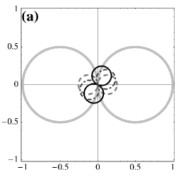
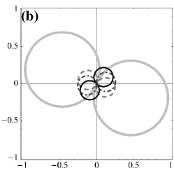
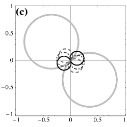
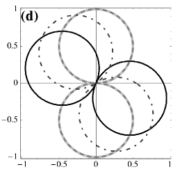
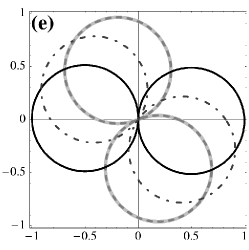
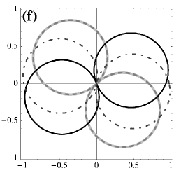
Figure 3: Polar plots of transmitted wave and incident wave polarization diagrams (namely, the dependence of $\left|\left(\mathbf{x}\otimes\mathbf{x}\right)\mathbf{H}\right|(\psi)$ where the vector $\mathbf{x}(\psi)=\mathbf{a}_{0}\cos\psi+\mathbf{b}_{0}\sin\psi$ rotates in the plane of interface) for a 27-layer fractal multilayer containing bi-isotropic layers with variable optical activity $\alpha$. The plots are given for off-peak [$\omega/\omega_{0}=1.0930$, (a-c)] and on-peak frequencies [$\omega/\omega_{0}=1.0938$, (d-f)]. The incident wave polarization varies between $0^{\circ}$ (a), $22.5^{\circ}$ (b), $45^{\circ}$ (c,f), $67.5^{\circ}$ (e), and $90^{\circ}$ (d).

As $\alpha$ increases, the transmission spectrum shows no modification whatsoever. The reflected wave does not change its polarization, either. The transmitted wave, however, exhibits polarization rotation. Figure 3 shows polarization diagrams for the transmitted wave for different input polarizations and for different values of $\alpha$, for two incident wave frequencies. These polarization diagrams is what a photodetector would register if placed behind a rotating analyzer in front of the output beam. It can be seen that this rotation is the same both at the transmission peak (figure 3d-f) and off-peak (figure 3a-c). So the polarization rotation is uniform, i.e., it has a similar manner at all frequencies and regardless of the spectral features. The angle of rotation can be written as

$$\phi=\sum_{j=1}^{N}\frac{\omega}{c}\alpha_{j}d_{j}$$ (14)

So it can be concluded that the influence of gyrotropy in this case is completely incoherent, i.e., totally independent of the geometrical properties of the multilayer.

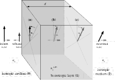
Figure 4: The illustration of spectrally uniform polarization rotation in bi-isotropic media. First, the incident wave hits the left interface (a). As the wave passes through the layer, its polarization is rotated (b). At the right interface (c) the wave is partially transmitted and partially back-reflected. As the back-reflected wave travels back, its polarization is rotated back (b), so it arrives at the left interface at exactly the same polarization as the incident wave (a). The process is repeated as this wave is partially reflected and partially transmitted again. (Double arrows denote propagation direction of the waves shown by the direction of their $\mathbf{H}$-vectors).

To illustrate this seemingly unexpected result, let us recall that in bi-isotropic media the polarization rotation direction is known to be reversed after normal-incidence reflection (so-called cross-polarized case described in [26]), in full accordance with the fact that the medium itself does not exhibit any specific directions. So the reflected part of the incident beam (see figure 4) will come to the initial interface ($0|1$) at its incident polarization, and this is true regardless of the number of multiple reflections taken into consideration. Similarly, at the second layer interface ($1|2$) all beams will have the same polarization, rotated with respect to the incident wave polarization according to (14). Since the transmittance is determined by interference effects resulting from multiple reflections, optical activity in a bi-isotropic layer cannot make any contribution except the above-mentioned polarization rotation (figure 4).

This explanation should hold regardless of the number of layers in a multilayer structure or of the structure geometry, because interference of multiply reflected beams should occur likewise at all the layer interfaces provided all the constituent layers are either isotropic or bi-isotropic. This was shown for periodic stacks in [29] and can also be derived from single-layer and single-interface results obtained in [24, 26].

To provide a consistent back-up for arbitrary NPD multilayers, let us calculate the evolution operator for a bi-isotropic layer. Starting with (4–5), one can immediately notice that for all the auxiliary vectors (5) the expressions in brackets are scalars and thus commute with $\mathbf{q}$, leaving the product $\mathbf{q}I$, which is identically zero. Remembering that $I\mathbf{q}^{\times}=\mathbf{q}^{\times}I=\mathbf{q}^{\times}$ and that the absence of absorption implies $\beta=-\alpha$, (4) can be reduced to

$$\mathbb{M}^{(b)}=\left[\begin{array}[]{cc}i\alpha\mathbf{q}^{\times}&\epsilon I\\ \mu I&i\alpha\mathbf{q}^{\times}\end{array}\right].$$ (15)

Taking the matrix exponential, one can, after some algebra, find the propagator to equal

$$\begin{array}[]{c}\mathbb{P}^{(b)}=\left[\begin{array}[]{cc}\cos(kd\sqrt{\epsilon\mu})P(\alpha)&\frac{i\epsilon}{\sqrt{\epsilon\mu}}\sin(kd\sqrt{\epsilon\mu})P(\alpha)\\ \frac{i\mu}{\sqrt{\epsilon\mu}}\sin(kd\sqrt{\epsilon\mu})P(\alpha)&\cos(kd\sqrt{\epsilon\mu})P(\alpha)\end{array}\right]\\ P(\alpha)\equiv\left[\cos(kd\alpha)I-\sin(kd\alpha)\mathbf{q}^{\times}\right]\end{array}$$ (16)

where $k\equiv\omega/c$.

The evolution operator for the isotropic layer with the same $\epsilon$, $\mu$, and $d$ can be found either by imposing $\alpha=0$ or directly from (8), which results in

$$\mathbb{P}^{(i)}=\left[\begin{array}[]{cc}\cos(kd\sqrt{\epsilon\mu})I&\frac{i\epsilon}{\sqrt{\epsilon\mu}}\sin(kd\sqrt{\epsilon\mu})I\\ \frac{i\mu}{\sqrt{\epsilon\mu}}\sin(kd\sqrt{\epsilon\mu})I&\cos(kd\sqrt{\epsilon\mu})I\end{array}\right].$$ (17)

We can see that every real-space block of both (16) and (17) has identical geometrical structure, with different coefficients for different components of the block vectors $\mathbb{W}$ in (6). This can be written as

$$\mathbb{P}^{(b)}=\left(\cos(kd\alpha)I-\sin(kd\alpha)\mathbf{q}^{\times}\right)\mathbb{L},\quad\mathbb{P}^{(i)}=I\mathbb{L}$$ (18)

where

$$\mathbb{L}=\left[\begin{array}[]{cc}\cos(kd\sqrt{\epsilon\mu})&\frac{i\epsilon}{\sqrt{\epsilon\mu}}\sin(kd\sqrt{\epsilon\mu})\\ \frac{i\mu}{\sqrt{\epsilon\mu}}\sin(kd\sqrt{\epsilon\mu})&\cos(kd\sqrt{\epsilon\mu})\end{array}\right].$$ (19)

Here one can note that the block matrix $\mathbb{L}$ consists of scalar quantities, so in terms of real space it is a coefficient matrix, which does not affect polarization properties. This essentially results from normal incidence. Also note that this coefficient matrix is the only part in $\mathbb{P}$ that depends on propagation phase $\varphi=\sqrt{\epsilon\mu}d\omega/c$.

Now let us show what such a propagator does to a normally incident vector $\mathbf{H}_{0}$. For simplicity and without loss of generality, we can assume $\mathbf{H}_{0}=H_{0}\mathbf{a}_{0}$, after which it can be seen from (13) that propagation in isotropic layer results in

$$\mathbb{W}=\mathbb{P}^{(i)}\mathbb{W}_{0}=H_{0}I\mathbb{L}\left[\begin{array}[]{c}\mathbf{a}_{0}\\ \frac{1}{n_{0}}\mathbf{a}_{0}\end{array}\right]=H_{0}\mathbb{L}\left[\begin{array}[]{c}1\\ \frac{1}{n_{0}}\end{array}\right]I\mathbf{a}_{0}=H_{0}\left[\begin{array}[]{c}t\\ t^{\prime}\end{array}\right]\mathbf{a}_{0}.$$ (20)

One can see that there is no polarization rotation. On the other hand, substituting the evolution operator of a bi-isotropic layer analogously yields

$$\mathbb{W}=\mathbb{P}^{(b)}\mathbb{W}_{0}=H_{0}\left[\begin{array}[]{c}t\\ t^{\prime}\end{array}\right]\left(\mathbf{a}_{0}\cos(kd\alpha)-\mathbf{b}_{0}\sin(kd\alpha)\right).$$ (21)

We can see that the polarization of the transmitted wave is rotated by the angle of $\phi=kd\alpha$, while the values of $t$ and $t^{\prime}$ (which contribute to the transmittance) remain the same. Besides, it can be stated that the propagator structure for the bi-isotropic layer in (18) explicitly contains the value of $\phi$.

To advance from a single layer to a multilayer structure, let us investigate what happens when propagators in the form (18) are multiplied. Naturally, we assume different $\varepsilon$, $\mu,$ $d$, and $\alpha$ (if any) for the two adjacent layers.

So, a product of two isotropic propagators reads

$$\mathbb{P}_{12}^{(ii)}=\mathbb{P}_{1}^{(i)}\mathbb{P}_{2}^{(i)}=\left(\mathbb{L}_{1}I\right)\left(\mathbb{L}_{2}I\right)=\left(\mathbb{L}_{1}\mathbb{L}_{2}\right)I=\mathbb{L}_{12}I$$ (22)

One can see that while the coefficient matrices $\mathbb{L}_{j}$ are multiplied (and hence the complex spectral effects are seen in isotropic multilayer structures), the real-space structure of the propagators remains proportional to $I$, i.e., polarization-independent.

Likewise, a product between isotropic and bi-isotropic propagators reads

$$\mathbb{P}_{12}^{(ib)}=\mathbb{P}_{1}^{(i)}\mathbb{P}_{2}^{(b)}=\mathbb{L}_{12}\left(\cos(kd_{2}\alpha_{2})I-\sin(kd_{2}\alpha_{2})\mathbf{q}^{\times}\right)$$ (23)

Again, the coefficient matrices are multiplied in the same manner, while real-space geometrical structure is preserved, so the angle of polarization rotation is unchanged compared to that for a single bi-isotropic layer.

Finally, taking a product between two bi-isotropic propagators, after some algebra we arrive at

$$\mathbb{P}_{12}^{(bb)}=\mathbb{L}_{12}\left(\cos(kd_{1}\alpha_{1}+kd_{2}\alpha_{2})I-\sin(kd_{1}\alpha_{1}+kd_{2}\alpha_{2})\mathbf{q}^{\times}\right).$$ (24)

So we see that the coefficient matrices are again multiplied likewise, and hence no change to the spectral properties provided that the same $\mathbb{L}_{1}$ and $\mathbb{L}_{2}$ are used in (22) and (24) – which is true if the corresponding layers have the same $\varepsilon$, $\mu$, and $d$. Looking at the geometrical structure of the propagators, we see that

$$\phi_{12}=\phi_{1}+\phi_{2}=\frac{\omega}{c}\left(\alpha_{1}d_{1}+\alpha_{2}d_{2}\right).$$ (25)

Certainly, as the propagator for any multilayer is built according to (7), and any multiplication according to (22–24) leads to the fact that spectra are independent of $\alpha$ while polarization rotation sums up, so (25) is directly generalized to (14). Therefore the reasoning applicable to a single bi-isotropic layer holds for any fractal structure (or, for that matter, for an arbitrarily designed binary multilayer composed of isotropic and bi-isotropic layers).

So far we have considered a linearly polarized incident wave. If the polarization is circular, it can be shown that change in effective refractive index does occur, however it does not manifest itself in the transmission spectra. Detailed explanation is provided in A.

To summarize, we have shown analytically that in multilayers consisting of isotropic and bi-isotropic layers in arbitrary combination the optical spectra are exactly the same as if there were no optical activity whatsoever, regardless of incident wave polarization. Instead, optical activity rotates the transmitted wave polarization, and the amount of this rotation is totally independent of the multilayer’s geometrical composition and is described by a simple equation (14).

This result can also be understood from the point of view that in a bi-isotropic multilayer system the multiple-reflected beams will interfere at each layer interface in exactly the same way as they do in the isotropic multilayer with the same $\epsilon$, $\mu$, and $d$. Since the optical spectra are determined by the nature of such interference, they are unmodified despite polarization rotation caused by each bi-isotropic layer and resulting in overall uniform polarization rotation.

Note that the analytical derivation in this case is rigorous and exact, without any assumptions on the values of parameters used. The only assumption regards the general applicability of local material equations (1), which restricts the layer thickness to the wavelength such that $d\gg 0.001\lambda$ [19] – a condition well met in the current state-of-the-art multilayers in the optical range.

In conclusion to this section, let us point out that the uniform and incoherent nature of the polarization plane rotation allows to use bi-isotropic materials to rotate polarization in devices with any geometry, without risk of additional interference effects. It can also be possible to combine spectral and polarization-rotating device in one multilayer, which should be beneficial for miniaturization of integrated optical components.

4 Gyrotropy and polarization-induced splitting

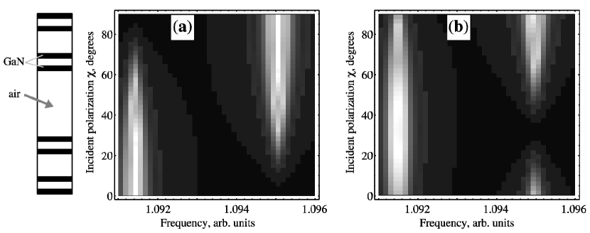
Figure 5: The dependence of transmittance on frequency and incident wave polarization for a 27-layer GaN/air fractal structure (inset) without (a) and with gyrotropy (b) with $\alpha=0.2$. Lighter areas denote higher transmittance.

Gradually complicating our structure, let us now consider a birefringent medium with a uniaxial permittivity tensor

$$\varepsilon=\epsilon_{o}+\left(\epsilon_{e}-\epsilon_{o}\right)\mathbf{c}\otimes\mathbf{c}$$ (26)

where, as noted before, $\varepsilon$ and $\epsilon$ are used to discriminate between tensor and scalar permittivity, respectively, and subscripts $o$ and $e$ stand for “ordinary” and “extraordinary”. A unit vector $\mathbf{c}$ determines the optical axis orientation. In multilayer structures under study, all uniaxial layers have similar orientation of $\mathbf{c}$ such that $\mathbf{cq}=0$. Without loss of generality we can assume $\mathbf{c}=\mathbf{b}_{0}$. As before, we assume no magnetic anisotropy, and isotropic optical activity.

Substituting (26) into (4–5) lets us arrive after some simple algebra at

$$\mathbb{M}^{(g)}=\left[\begin{array}[]{cc}i\alpha\mathbf{q}^{\times}&\varepsilon I+iQ\mu_{q}\mathbf{q}^{\times}\varepsilon\mathbf{q}\otimes\mathbf{q}^{\times}\mathbf{q}\varepsilon I\\ \mu I&i\alpha\mathbf{q}^{\times}\end{array}\right]=\left[\begin{array}[]{cc}i\alpha\mathbf{q}^{\times}&\varepsilon I\\ \mu I&i\alpha\mathbf{q}^{\times}\end{array}\right].$$ (27)

Without optical activity ($\alpha=0$) and within our assumptions ($\mathbf{c}=\mathbf{b}_{0}$) the propagator can be found to equal

$$\mathbb{P}^{(a)}=\mathbb{L}_{o}\mathbf{a}_{0}\otimes\mathbf{a}_{0}+\mathbb{L}_{e}\mathbf{b}_{0}\otimes\mathbf{b}_{0}$$ (28)

where

$$\mathbb{L}_{j} = \left[\begin{array}[]{cc}\cos(kd\sqrt{\epsilon_{j}\mu})&\frac{i\epsilon_{j}}{\sqrt{\epsilon_{J}\mu}}\sin(kd\sqrt{\epsilon_{j}\mu})\\ \frac{i\mu}{\sqrt{\epsilon_{j}\mu}}\sin(kd\sqrt{\epsilon_{j}\mu})&\cos(kd\sqrt{\epsilon_{j}\mu})\end{array}\right],\quad j=o,e.$$ (31)

It can be easily seen that such a layer is able to exhibit polarization-induced peak splitting in the spectrum. Indeed, when a field vector is oriented along $\mathbf{a}_{0}$ (or, more generally speaking, perpendicular to $\mathbf{c}$), it will only interact with one term in the propagator, namely, the one containing $\mathbb{L}_{o}$, and will propagate exactly as if all uniaxial layers were isotropic with $\epsilon=\epsilon_{o}$ [compare (19) and (31)]. Similarly, when a field vector is oriented along $\mathbf{b}_{0}$ (parallel to $\mathbf{c}$), the same would be true for $\mathbb{L}_{e}$, and again all uniaxial layers will effectively be isotropic, this time with $\epsilon=\epsilon_{e}$. So, one can see that if the incident wave is polarized along either of the eigenvectors of $\mathbb{P}$ (it is then called an eigenwave), it will propagate in exactly the same way as if all uniaxial layers were isotropic with some effective refractive index. Hence the spectra will be similar in shape, the only difference associated with a change in effective $\epsilon$, which in turn causes all spectral features to shift in frequency.

Unfortunately, in presence of optical activity the tensorial nature of $\varepsilon$ results in a very complicated structure of the propagator, which, while capable of being evaluated symbolically, is nearly useless for further analysis.

It can be shown, however, that if we assume both $\alpha$ and $\delta\epsilon\equiv\frac{1}{2}\left|\epsilon_{e}-\epsilon_{o}\right|$ to be small, an approximate model propagator can be used. The details on its derivation and applicability are covered in  B. Reduced with respect to $\delta\epsilon$ with the product $\alpha\delta\epsilon$ neglected, it reads

$$\mathbb{P}^{(g)}\approx\mathbb{L}\left(\cos(kd\alpha)I-\sin(kd\alpha)\mathbf{q}^{\times}\right)+\delta\epsilon\mathbb{L}^{\prime}\left(\mathbf{a}_{0}\otimes\mathbf{a}_{0}-\mathbf{b}_{0}\otimes\mathbf{b}_{0}\right).$$ (32)

Here the coefficient matrix $\mathbb{L}$ is the same as that for isotropic media [compare (56) and (19)] if we substitute $\epsilon\equiv\frac{1}{2}\left(\epsilon_{e}+\epsilon_{o}\right)$, i.e., if an average between ordinary and extraordinary dielectric constant is used as an effective value of $\epsilon$. The coefficient matrix $\mathbb{L}^{\prime}$ is explicitly written as (57).

On the other hand, one can reduce the same model propagator with respect to $\alpha$, in which case

$$\mathbb{P}^{(g)}\approx\mathbb{L}_{o}\mathbf{a}_{0}\otimes\mathbf{a}_{0}+\mathbb{L}_{e}\mathbf{b}_{0}\otimes\mathbf{b}_{0}-kd\alpha\mathbb{L}\mathbf{q}^{\times},$$ (33)

where the matrices $\mathbb{L}_{o}$ and $\mathbb{L}_{e}$ are the same as those without gyrotropy [see (28–31)], and the additional coefficient matrix $\mathbb{L}$ given in (56) is the same as for isotropic case in (19).

Looking at (32) and (33), one can see that even within the bounds of the approximation used, the behavior of the multilayer in question changes dramatically. Compared to a bi-isotropic evolution operator (18), there is a symmetric addition proportional to $\delta\epsilon$, which causes perturbation to polarization plane rotation, making the propagator polarization-sensitive. Hence, the propagator multiplication is no longer described by (24), and the angle of rotation becomes dependent on the incident wave polarization.

Compared to a birefringent evolution operator (28), there is an antisymmetric addition proportional to $\alpha$ (and, more generally, this $\alpha$ comes from decomposition of $\sin kd\alpha$). We know from (18) that such a term in the propagator is responsible for polarization plane rotation.

As it is not easy to decide in favor of one on these two interpretations, it is safe to assume that one layer made of material in question will exhibit polarization rotation combined (more or less on equal terms) with spectral properties of birefringent multilayer structures.

Numerical results show that this is indeed the case. For simulation, the same GaN/air fractal multilayer as in the previous section was used (shown again in figure 5), but without rendering the GaN layers isotropic. Optical activity was likewise artificially introduced into GaN, $\alpha$ ranging up to $0.2$.

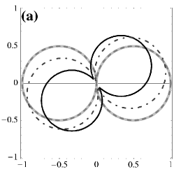
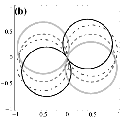
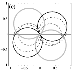
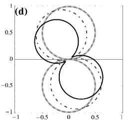
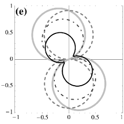
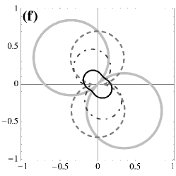
Figure 6: Polar plots of transmitted wave and incident wave polarization diagrams (the same as in Fig. 3) for a 27-layer fractal multilayer containing birefringent layers with variable isotropic optical activity $\alpha$. The plots are given for the same incident wave polarizations for both polarization-split peaks [$\omega/\omega_{0}=1.0923$ (a-c), $\omega/\omega_{0}=1.0938$ (d-f)]. The incident wave polarization varies between $0^{\circ}$ (a), $22.5^{\circ}$ (b), $45^{\circ}$ (c,f), $67.5^{\circ}$ (e), and $90^{\circ}$ (d).

As one can see in figure 5, there is no change in the nature of polarization-induced splitting, and the frequencies of the doublet components are not changed, either. This agrees with (33) where we see the coefficient matrices $\mathbb{L}_{o}$ and $\mathbb{L}_{e}$ to be the same regardless of optical activity. However, the sensitivity of splitting to input polarization has been modified dramatically. Without gyrotropy there is a clear symmetric picture with peak maxima corresponding to the cases when the incident wave coincides with one of the eigenpolarizations (figure 5a). When gyrotropy is present, the peak maxima become shifted by about 30 degrees, and the transmittance at maximum does not reach unity (figure 5b).

To proceed with in-depth analysis, let us look at the transmitted wave polarization (figure 6). The diagrams are plotted for the same incident wave polarizations as in figure 3 at the frequencies of polarization-split doublet. One can see immediately that the transmitted wave polarization is modified considerably if gyrotropy is present. The structure still works as a polarizer in a sense that at both peaks the transmitted wave is always polarized similarly for any input polarization. This can be seen by comparing the graphs in figure 6a-c as well as in figure 6d-f. However, the output polarization states are found to depend on the optical activity strength present. This dependence mainly manifests itself as rotation, so the output polarization states remain visibly orthogonal for the two peaks. However, besides the change in orientation there is also a change in ellipticity, as can best be seen in figure 6f.

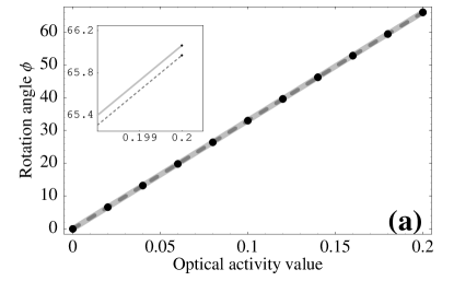
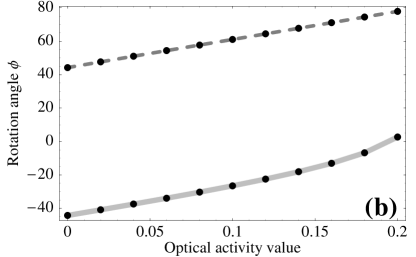
Figure 7: The dependence of polarization rotation angle $\phi$ on the value of $\alpha$ for isotropic (a) and birefringent (b) multilayer structure. The incident wave polarization is according to Fig. 6c for the split peak frequencies $\omega/\omega_{0}=1.0923$ (dashed) and $\omega/\omega_{0}=1.0938$ (solid). The inset shows a slight difference in the slope for the two lines according to (14).

It is also worth noting that the character of polarization rotation in this case is completely different from what was observed in the previous section. This difference is best seen comparing figure 3c,f and figure 6c,f, when the same incident wave polarization is considered, and plotting the angle of rotation $\phi$ versus optical activity $\alpha$ (figure 7). In the bi-isotropic case the rotation is always with respect to incident wave, it is independent of the structure’s geometrical or spectral features, so $\phi$ is almost equal for resonant and off-resonant frequencies, exhibiting only a slight frequency variation according to (14) (figure 7a).

In the case when isotropic optical activity is added to birefringence, the dominant feature is polarization-induced splitting, its polarization properties subject to modification due to gyrotropy. This happens in a multilayer because splitting (along with all spectral features) is resonant and the more layers there are in a multilayer, the more pronounced the peaks are. On the other hand, gyrotropy-induced rotation in (32) only weakly increases with the number of layers. So, the rotation occurs with respect to eigenpolarizations of the birefringent medium. The angle of rotation $\phi$ is thus strongly dependent on frequency, exhibiting a change of $90^{\circ}$ over a very small change ($\Delta\omega/\omega_{0}=0.0015$) between two polarization-split peaks (figure 7b). The dependence $\phi(\alpha)$ itself no longer conforms to (14) and even exhibits a slight nonlinearity, apparently connected to the emerging ellipticity in output polarization (see figure 6f).

It may appear at first that this change of output polarization should correspond to the change of polarization eigenstates in gyrotropic media. However, in this case one would expect exactly the same propagator structure as in (28) with $\mathbf{a}_{0}$ and $\mathbf{b}_{0}$ replaced with elliptical eigenvectors, which could have been recoverable from figure 6. This, however, is not straightforward (see A), and this would also contradict with the structure in (33) where a term proportional to $d\alpha$ is present. Together with an additional term in (32) this means that eigenvectors should be thickness-dependent. This cannot happen since eigenvectors of $\mathbb{P}$ are the same as those of $\mathbb{M}$, which depends only on material parameters.

Indeed, if only change of eigenpolarizations were involved here, then gyrotropy would leave unchanged the Malus-like dependence of transmittance on input polarization, with respect to rotated output polarization states – quite contrary to what is seen in figure 6c where the output and input waves are almost mutually perpendicular in polarization, yet the transmittance is near unity. So one may guess that there should be an interplay between “bi-isotropic-like” uniform polarization rotation and gyrotropy-induced change of eigenpolarizations. The exact nature of this interplay is yet to be understood.

To summarize this section, we have found out that isotropic optical activity added to a birefringent multilayer structure influences both the transmission spectra and the transmitted wave polarization. However, the modification of the spectra can be seen in the change of polarization sensitivity. The nature of polarization-induced splitting, the frequencies of split components, and the orthogonality of output polarization for these components remains unaltered.

The results obtained can be used to control the output polarization of a splitter based on an NPD multilayer with anisotropic layers. This control occurs without any modification to the splitter frequency characteristics. This is definitely of interest in the design of integrated optical polarizers, as both polarization directions can be rotated without having to physically re-orient the multilayer. Again, fractal structures are geometrically preferable as NPD structures because peak multiplicity allows polychromatic filtering properties. This can facilitate both multiple-channel polarization separators and split component matching, which can in turn be promising in applications.

5 Conclusions and outlook

In conclusion, we have analyzed the influence of isotropic optical activity, the simplest kind of gyrotropy, on the spectral and polarization properties of deterministic non-periodic (in particular, fractal) multilayer structures. In isotropic case, we have shown numerically and analytically that optical activity does not cause any change in the transmission spectrum, but rather leads to a uniform polarization rotation. It is independent of the structure geometry and can be described by (14). In birefringent case, we have shown that the frequencies of polarization-split doublet do not change. However, both the output polarization and the value of transmittance at peak frequencies do depend on the strength of gyrotropy. In more complicated cases, when gyrotropy-related terms are expected to cross-couple with $\varepsilon$ and $\mu$ in the single-layer characteristic operator (4–5), more significant modification of the spectra can be expected, e.g., changes of resonant peak locations.

The results obtained are characteristic to any structure geometry that facilitates sharp resonance peaks located in a band gap, as is the case with many deterministic non-periodic media. Fractal geometry considered here allows the effects to be manifest in the desire frequency range with desired peak multiplicity. Among other notable geometries one can also name single- and multiple-cavity Fabry-Pérot resonators embedded into a periodic multilayer.

The effects observed can be used in the design of frequency-selective, compact devices for polarization-sensitive integrated optics. This particularly concerns mono- and polychromatic absorptionless polarizers with controlled output polarization. Devices that rotate the polarization of output beam with respect to the input are also possible. Note, however, that in this paper no account was taken for present-day experimental or technological applicability of the results obtained. Also note that the combination of parameters described in Section 4 is not among those naturally occurring in crystals (though it may be possible in nanocomposites). Nevertheless, this combination is very useful illustratively, since it allows analytical treatment and so can be used as a landmark of what will happen if we complicate the system further.

There is a broad range of problems to be addressed within the scope of extending the present research. First and foremost, it appears fruitful to investigate more complicated cases of optical anisotropy and gyrotropy. This is especially relevant is two cases. First, of interest are materials with properties subject to external tuning, e.g., liquid crystals or Pockels, Faraday, or Kerr media. Secondly, as was mentioned above, of importance are anisotropic and/or gyrotropic materials which can be readily used in multilayer micro- and nanostructure fabrication. Since the numerical techniques used in this paper are based on the general material equations (1), it appears possible to rigorously allow for all kinds of anisotropy and gyrotropy, as well as to account for polarization effects during wave propagation. This paper demonstrates that analytical or semi-analytical treatment is possible using symbolic computation techniques. A thorough classification of spectral and polarization-related effects resulting from anisotropy and/or gyrotropy according to different crystallographic symmetries existent in nature is worthwhile, too.

Other areas of extending this paper are also apparent. Namely, it is interesting to find out what happens in NPD multilayers containing anisotropic or gyrotropic layers of the same material but different spatial orientation. In addition, it also appears promising to combine materials with various optical properties in different parts of the same NPD multilayer. Since such structures generally tend to exhibit eigenmodes with distinct localization patterns, one may expect that by introducing different materials into different localization regions one can produce devices with unusual and largely tunable spectral dependencies of optical properties.

Appendix A Bi-isotropic media and circular polarization

From the reasoning of Section 3, one may conceive that bi-isotropic media allegedly do not discriminate between left-handed and right-handed circular polarization, while it is commonly known (see [27, 33]) that on the contrary, change of effective refractive index occurs. Here we would like to explain in detail how and why this effective index change does not cause any polarization splitting.

We take a single bi-isotropic layer and analyze what happens to a circularly polarized incident wave. Starting with (21), we can see that in this case ($\phi\equiv kd\alpha$)

$$\mathbf{H}_{0}^{+}=H_{0}(\mathbf{a}_{0}+i\mathbf{b}_{0}),$$

$$\mathbb{W}^{+} = H_{0}\mathbb{L}\left[\begin{array}[]{c}1\\ \frac{1}{n_{0}}\end{array}\right]\left[\left(\cos\phi+i\sin\phi\right)\mathbf{a}_{0}+i\left(\cos\phi+i\sin\phi\right)\mathbf{b}_{0}\right]=$$ (36)

$$= \mathbb{L}\left[\begin{array}[]{c}1\\ \frac{1}{n_{0}}\end{array}\right]\mathbf{H}_{0}^{+}e^{i\phi}.$$ (39)

We can see that there is no change of polarization but rather a change of phase for the transmitted wave with respect to that for isotropic layer. The value of this change is $\phi$. If one reverses the direction of circular polarization, one gets

$$\mathbf{H}_{0}^{-}=H_{0}(\mathbf{a}_{0}-i\mathbf{b}_{0}),$$

$$\mathbb{W}^{-} = H_{0}\mathbb{L}\left[\begin{array}[]{c}1\\ \frac{1}{n_{0}}\end{array}\right]\left[\left(\cos\phi-i\sin\phi\right)\mathbf{a}_{0}+i\left(-\cos\phi+i\sin\phi\right)\mathbf{b}_{0}\right]=$$ (42)

$$= \mathbb{L}\left[\begin{array}[]{c}1\\ \frac{1}{n_{0}}\end{array}\right]\mathbf{H}_{0}^{-}e^{-i\phi}.$$ (45)

As can be noticed, the change of phase is different in this case. A conventional approach with bulk bi-isotropic media is to combine this phase shift $\phi$ with propagation phase $\varphi=kd\sqrt{\epsilon\mu}$. This results in a change in effective refractive index, such that [27]

$$n_{\textnormal{eff}}^{\pm}=n_{0}\pm\delta n=\sqrt{\epsilon\mu}\pm\alpha.$$ (46)

However, our studies show that such an approach can yield misleading results when applied even to a single layer. A straightforward conclusion of the effective index concept would be that the layer, and even more so the multilayer structure, should become sensitive to the orientation of circular polarization. Indeed, as spectral features strongly depend on $n$, the difference in $n_{\textnormal{eff}}$ should result in the difference in the spectra, causing polarization-induced splitting with respect to circular eigenpolarizations.

However, this contradicts with both numerical and analytical results. Indeed, note first that the phase change in (36–42), even if included in $\mathbb{L}$, does not contribute to transmittance. Further, considering a multilayer composed of $N$ isotropic and bi-isotropic layers, one can use (22–24) to see that

$$\mathbb{W}^{\pm}=\mathbb{L}_{1}\mathbb{L}_{2}\cdots\mathbb{L}_{N-1}\mathbb{L}_{N}\left[\begin{array}[]{c}1\\ \frac{1}{n_{0}}\end{array}\right]\mathbf{H}_{0}\exp(\pm\phi_{1}\pm\phi_{2}\pm\ldots\pm\phi_{N}).$$ (47)

Since transmission spectrum is determined by the matrix product in (47), which is polarization-independent, bi-isotropy in any of the constituent layers cannot lead to polarization-induced splitting. Instead, it contributes to an overall uniform phase change – similar to a uniform polarization rotation in the case of linear input polarization.

This example is a good confirmation of the fact that the refractive index itself is no longer straightforward nor safe to use once complex optical media are involved. Indeed, an effective refractive index for a certain eigenpolarization essentially means that a wave with this polarization propagates as if the medium were isotropic. But it can only be true if the wave polarization is never changed during propagation. In homogeneous media of any kind, it is always true by definition of an eigenwave [33] – so it is enough to make sure that the incident wave is properly polarized, which is what is conventionally assumed.

However, in inhomogeneous media this is no longer enough. Even in a multilayer the layer interfaces can and do introduce polarization coupling between eigenwaves. And this is exactly what occurs in a bi-isotropic layer – both layer interfaces serve as perfect couplers between eigenpolarizations, reversing the polarization after each reflection. (This cross-coupling is mentioned in [26] and is due to the fact that right- or left-handedness of a circularly-polarized wave is determined by the sign of the vector product $i\mathbf{n}[\mathbf{H}\times\mathbf{H}^{*}]$ [22], and during Fresnel reflection in our case $\mathbf{n}\rightarrow-\mathbf{n}$, $\mathbf{H}\rightarrow r\mathbf{H}$, $r$ being real). As such, even in the case of one layer, even in the case of normal incidence and axial symmetry of the system, the wave initially polarized along one of the eigenwaves does not retain its polarization during propagation. Therefore the resulting spectral properties even of one layer differs greatly from what would have happened if one blindly used the effective index concept suitable for homogeneous media.

Appendix B Evolution operator for a uniaxial, isotropically optically active layer

Here we would like to show in detail the way we have derived the model propagator for a uniaxially birefringent layer with isotropic gyrotropy to be used in (32) and (33).

The main difficulty in evaluating the propagator directly from (27) consists in the fact that eigenvectors of such a matrix are complex elliptical vectors whose orientation and ellipticity depend on numerical relations between $\epsilon_{o}$, $\epsilon_{e}$, and $\alpha$, and layer interfaces even for one layer will play a role not clearly understood (see A). The expression for $\mathbb{P}$ becomes excessively complex to be analyzed successfully.

One of the ways out would be to construct approximations assuming that $\alpha$ and $\left|\epsilon_{e}-\epsilon_{o}\right|$ are small quantities. However, such approximation has to be done carefully, since while these quantities are small enough indeed, they appear in the propagator multiplied by $d\omega/c$, and the resulting phases are no longer infinitesimal. So it can be misleading to straightforwardly suppose $\left|\varepsilon_{e}-\varepsilon_{o}\right|^{2}=0=\alpha^{2}$.

Instead, what can be done is to analyze several orders of Taylor series for $\mathbb{P}$ in order to recover how the Taylor decomposition can fold back into trigonometric expressions so as to produce the same Taylor series up to a certain order. The result of this operation is what we call here the model propagator. Reduced to a $4\times 4$ form [see the footnote for (16)], it reads

$$\mathbb{P}^{(g)}=\left[\begin{array}[]{cc}A&B\\ C&D\end{array}\right],$$ (48)

$$A\approx\left[\begin{array}[]{cc}\cos kd\sqrt{\mu\epsilon_{o}}\cos\phi&\cos kd\sqrt{\mu\epsilon^{\prime}}\left(1-\Delta\right)\sin\phi\\ -\cos kd\sqrt{\mu\epsilon^{\prime}}\left(1+\Delta\right)\sin\phi&\cos kd\sqrt{\mu\epsilon_{e}}\cos\phi\end{array}\right],$$ (49)

$$D\approx\left[\begin{array}[]{cc}\cos kd\sqrt{\mu\epsilon_{o}}\cos\phi&\cos kd\sqrt{\mu\epsilon^{\prime}}\left(1+\Delta\right)\sin\phi\\ -\cos kd\sqrt{\mu\epsilon^{\prime}}\left(1-\Delta\right)\sin\phi&\cos kd\sqrt{\mu\epsilon_{e}}\cos\phi\end{array}\right],$$ (50)

$$B\approx\left[\begin{array}[]{cc}\frac{i\epsilon}{\sqrt{\mu\epsilon_{e}}}\sin kd\sqrt{\mu\epsilon_{o}}\cos\phi&\frac{i\epsilon}{\sqrt{\epsilon\mu}}\sin kd\sqrt{\epsilon\mu}\sin\phi\\ -\frac{i\epsilon}{\sqrt{\epsilon\mu}}\sin kd\sqrt{\epsilon\mu}\sin\phi&\frac{i\epsilon}{\sqrt{\mu\epsilon_{o}}}\sin kd\sqrt{\mu\epsilon_{e}}\cos\phi\end{array}\right],$$ (51)

$$C\approx\left[\begin{array}[]{cc}\frac{i\epsilon}{\sqrt{\mu\epsilon_{o}}}\sin kd\sqrt{\mu\epsilon_{o}}\cos\phi&\frac{i\mu}{\sqrt{\epsilon\mu}}\sin kd\sqrt{\epsilon\mu}\sin\phi\\ -\frac{i\mu}{\sqrt{\epsilon\mu}}\sin kd\sqrt{\epsilon\mu}\sin\phi&\frac{i\mu}{\sqrt{\mu\epsilon_{e}}}\sin kd\sqrt{\mu\epsilon_{e}}\cos\phi\end{array}\right],$$ (52)

In order to simplify off-diagonal terms to the maximum possible extent, we have substituted $\epsilon_{o}\equiv\epsilon-\delta\epsilon$, $\epsilon_{e}\equiv\epsilon+\delta\epsilon$. Also, $\Delta\equiv\frac{1}{2}\sin(\delta\epsilon/\epsilon)$ and $\epsilon^{\prime}\equiv\epsilon\left(1-\delta\varphi\right)$ where $\delta\varphi\equiv\delta\epsilon(kd\sqrt{\epsilon\mu})^{-2}$, and as before, $\phi=kd\alpha$.

It can be confirmed that the propagator constructed according to (48–52) yields the same Taylor decomposition as the real matrix exponential when the terms up to $\alpha^{2}$ and $\delta\epsilon^{2}$ are preserved.

Certainly, the propagator of (48–52) is by no means a true form of the evolution operator; it is not even an approximation in the strict sense – rather, it is an expression, which yields the same approximation. Hence it can be used as an approximate model of a real gyrotropic layer. The fact that it is trigonometrical allows us to analyze such phenomena as polarization plane rotation and birefringence, reverting to decomposition only when and where needed. The only apparent limitation of this approach is that we should not decompose (49–52) to more than the second order with respect to $\alpha$ and $\delta\epsilon$.

This kept in mind, one can take Taylor in square roots with respect to $\delta\epsilon$ and neglect the product $\alpha\delta\epsilon$ (which is essentially a quadratic term). This yields ($\varphi\equiv kd\sqrt{\epsilon\mu}$)

$$\begin{array}[]{l}A=D\approx P\cos\varphi+\delta\epsilon\lambda_{d}S\sin\varphi,\\ B\approx\frac{i\epsilon}{\sqrt{\varepsilon\mu}}\left[P\sin\varphi-\delta\epsilon\left(\lambda_{od}+\lambda^{\prime}\right)S\cos\varphi\right],\\ C\approx\frac{i\mu}{\sqrt{\epsilon\mu}}\left[P\sin\varphi+\delta\epsilon\left(\lambda_{od}-\lambda^{\prime}\right)S\cos\varphi\right],\\ P\equiv I\cos\phi-\mathbf{q}^{\times}\sin\phi,\quad S\equiv\mathbf{a}_{0}\otimes\mathbf{a}_{0}-\mathbf{b}_{0}\otimes\mathbf{b}_{0}\end{array}$$ (53)

where the subscripts $d$ and $od$ stand for “diagonal” and “off-diagonal”, and

$$\lambda_{d}=\frac{kd\mu}{2\sqrt{\epsilon\mu}},\quad\lambda_{od}=\frac{kd\sqrt{\epsilon\mu}}{2\epsilon},\quad\lambda^{\prime}=\frac{1}{2\epsilon}.$$ (54)

Therefore one can rewrite (53–54) in the form analogous to (18) and (28):

$$\mathbb{P}^{(g)}\approx\mathbb{L}\left(I\cos\phi-\mathbf{q}^{\times}\sin\phi\right)+\delta\epsilon\mathbb{L}^{\prime}\left(\mathbf{a}_{0}\otimes\mathbf{a}_{0}-\mathbf{b}_{0}\otimes\mathbf{b}_{0}\right)$$ (55)

Eq. (55) is used in the text as (32). The coefficient matrices are

$$\mathbb{L}=\left[\begin{array}[]{cc}\cos\varphi&\frac{i\epsilon}{\sqrt{\epsilon\mu}}\sin\varphi\\ \frac{i\mu}{\sqrt{\epsilon\mu}}\sin\varphi&\cos\varphi\end{array}\right],$$ (56)

$$\mathbb{L}^{\prime}=\left[\begin{array}[]{cc}\frac{kd\mu}{2\sqrt{\epsilon\mu}}\sin\varphi&-\frac{i\epsilon}{\sqrt{\epsilon\mu}}\left(\frac{kd\sqrt{\epsilon\mu}}{2\epsilon}+\frac{1}{2\epsilon}\right)\cos\varphi\\ \frac{i\mu}{\sqrt{\epsilon\mu}}\left(\frac{kd\sqrt{\epsilon\mu}}{2\epsilon}-\frac{1}{2\epsilon}\right)\cos\varphi&\frac{kd\mu}{2\sqrt{\epsilon\mu}}\sin\varphi\end{array}\right].$$ (57)

On the other hand, one can take Taylor of (49–52) in another manner, excluding the propagation phase $\varphi$ rather than the polarization plane rotation $\phi$ from decomposition. Making use of the fact that

$$\frac{i\epsilon}{\sqrt{\mu\left(\epsilon\mp\delta\epsilon\right)}}\sin kd\sqrt{\mu\left(\epsilon\pm\delta\epsilon\right)}\simeq\frac{i\left(\epsilon\pm\delta\epsilon\right)}{\sqrt{\mu\left(\epsilon\pm\delta\epsilon\right)}}\sin kd\sqrt{\mu\left(\epsilon\pm\delta\epsilon\right)}+O\left(\delta\epsilon^{2}\right)$$

and likewise neglecting $\alpha\delta\epsilon$, we obtain

$$\begin{array}[]{l}A=D\approx\mathbf{a}_{0}\otimes\mathbf{a}_{0}\cos\varphi_{o}+\mathbf{b}_{0}\otimes\mathbf{b}_{0}\cos\varphi_{e}-\alpha kd\cos\varphi\mathbf{q}^{\times},\\ B\approx\frac{i\epsilon_{o}}{\sqrt{\epsilon_{o}\mu}}\mathbf{a}_{0}\otimes\mathbf{a}_{0}\sin\varphi_{o}+\frac{i\epsilon_{e}}{\sqrt{\epsilon_{e}\mu}}\mathbf{b}_{0}\otimes\mathbf{b}_{0}\sin\varphi_{e}-\frac{i\epsilon}{\sqrt{\varepsilon\mu}}\alpha kd\sin\varphi\mathbf{q}^{\times},\\ C\approx\frac{i\mu}{\sqrt{\varepsilon_{o}\mu}}\mathbf{a}_{0}\otimes\mathbf{a}_{0}\sin\varphi_{o}+\frac{i\mu}{\sqrt{\varepsilon_{e}\mu}}\mathbf{b}_{0}\otimes\mathbf{b}_{0}\sin\varphi_{e}-\frac{i\mu}{\sqrt{\varepsilon\mu}}\alpha kd\sin\varphi\mathbf{q}^{\times}.\end{array}$$ (58)

Here, naturally, $\varphi_{o}\equiv kd\sqrt{\varepsilon_{o}\mu}$, $\varphi_{e}\equiv kd\sqrt{\varepsilon_{e}\mu}$. Thus, isolating the real-space structure on analogy with (55), we have

$$\mathbb{P}^{(g)}\approx\mathbb{L}_{o}\mathbf{a}_{0}\otimes\mathbf{a}_{0}+\mathbb{L}_{e}\mathbf{b}_{0}\otimes\mathbf{b}_{0}-kd\alpha\mathbb{L}\mathbf{q}^{\times}.$$ (59)

This formula is used in the text as (33). The coefficient matrices $\mathbb{L}_{a}$ and $\mathbb{L}_{b}$ are identical to those in (31). The antisymmetric term contains the same matrix $\mathbb{L}$ as in (56).

References

References

- [1] Joannopouos J D, Meade R D and Winn J. N 1995 Photonic Crystals: Molding the Flow of Light (Princeton: Princeton University Press)
- [2] Sakoda K 2001 Optical Properties of Photonic Crystals (Berlin: Springer)
- [3] Kohmoto M, Sutherland B and Iguchi K 1987 Phys. Rev. Lett. 58 2436–8
- [4] Maci�E 1998 Appl. Phys. Lett. 73 3330–2
- [5] Vasconcelos M S, Albuquerque E L and Mariz A M 1999 J. Phys.: Cond. Matt. 10 5839–49
- [6] Lavrinenko A V, Zhukovsky S V, Sandomirskii K S and Gaponenko S V 2003 Phys. Rev. E 65 036621
- [7] Zhukovsky S V, Lavrinenko A V and Gaponenko S V 2002 Proc. SPIE vol 4705 pp 121–8
- [8] Zhukovsky S V, Lavrinenko A V and Gaponenko S V 2004 Europhys. Lett. 66, 455–61
- [9] Liu Z, Lin Z and Chui S T 2004 Phys. Rev. B 69 115402
- [10] Mandatori A, Sibilia C, Bertolotti M, Zhukovsky S, Haus J W and Scalora M 2004 Phys. Rev. B 70 165107
- [11] Mandatori A, Sibilia C, Bertolotti M, Zhukovsky S and Gaponenko S V 2005 J. Opt. Soc. Am. B 22 1785–92
- [12] Makarov D G, Danilov V V and Kovalenko V F 2004 Phys. Stat. Sol. 201 130–8
- [13] Borzdov A N 1997 Proc. Bianisotropics 1997 (Glasgow) (Glasgow: Glasgow Univ. Publication) pp 145–8
- [14] Borzdov A N 1999 Electromagnetics 19 501–12
- [15] Borzdov A N 2000 Bianisotropics 2000: Proc. 8th Int. Conf. on Electromagnetics of Complex Media (Lisbon: Lisbon Technical Univ. Publication) pp 135–8
- [16] Chongjun J, Bai Q, Miao Y and Ruhu Q 1997 Opt. Commun. 142 179–83
- [17] Psarobas I E, Stefanou N and Modinos A 1999 J. Opt. Soc. Am. A 16 343–7
- [18] Zhukovsky S V 2003 Proc. 5th Int. Conf. on Transparent Optical Networks and 2nd European Symp. on Photonic Crystals vol 1 (Warsaw: Inst. of Telecommunications) pp 326–9
- [19] Fedorov F I 1976 Theory of gyrotropy (Minsk: Nauka)
- [20] Fedorov F I 2004 Optics of anisotropic media, 2nd ed (Moscow: Editorial URSS)
- [21] Barkovskii L M, Borzdov G N and Lavrinenko A V 1987 J. Phys. A: Math. Gen. 20 1095–106
- [22] Fedorov F I 1958 Theory of elastic waves in crystals (New York: Plenum)
- [23] Lakhtakia A, Varadan V V and Varadan V K 1988 J. Opt. Soc. Am. A 5 175–84
- [24] Lakhtakia A, Varadan V V and Varadan V K 1989 J. Opt. Soc. Am. A 6 1675–81
- [25] Jaggard D L, Engheta N, Kowarz M W, Pelet P, Liu J C and Kim Y 1989 IEEE Trans. Ant. Propag. 37 1447–52
- [26] Jaggard D L and Sun X 1992 J. Opt. Soc. Am. A 9 804–13
- [27] Georgieva E 1995 J. Opt. Soc. Am. A 12 2203–11
- [28] Slepyan G Ya, Gurevich A V and Maksimenko S A 1995 Phys. Rev. E 51 2543–9
- [29] Flood K M and Jaggard D L 1996 J. Opt. Soc. Am. A 13 1395–406
- [30] Cory H and Rosenhouse I 1997 Electromagnetics 17 317–41
- [31] Becchi M and Galatola P 1999 Europ. Phys. J. B 8 399–404
- [32] Kim K, Lee D–H and Lim H 2005 Europhys. Lett. 69 207–13
- [33] Barkovskii L M, Borzdov G N and Fedorov F I 1990 J. Mod. Opt. 37 85–97