Using Qubits to Measure Fidelity in Mesoscopic Systems

Abstract

We point out the similarities in the definition of the ‘fidelity’ of a quantum system and the generating function determining the full counting statistics of charge transport through a quantum wire and suggest to use flux- or charge qubits for their measurement. As an application we use the notion of fidelity within a first-quantized formalism in order to derive new results and insights on the generating function of the full counting statistics.

I Introduction

Mesoscopic devices exhibit an extraordinary rich and complex behavior; their proper characterization has sparked numerous ideas. Two such basic mesoscopic characteristics are the stability of a quantum system peres , nowadays compiled under the terms ‘fidelity’ or ‘Loschmidt echo’, and the full counting statistics of charge transport, expressed through the generating function for the distribution of charge transmitted across a quantum wire ll23 . Here, we combine these items with recent efforts aiming at the physical realization of quantum bits, the controllable quantum two-level systems which are the basic elements of a quantum computer nielsonchuang ; by now, a number of devices have been realized in the laboratory, among them particular solid-state implementations such as flux- chiorescu or charge- vion qubits which are easy to couple to. The purpose of this letter is three-fold: i) to draw attention to the equivalence between the fidelity of a quantum system and the generating function for the full counting statistics, two quantities which have been conceived to be unrelated so far. This insight generalizes the concept of fidelity to mixed states and many-particle systems. ii) to suggest measuring the fidelity/full counting statistics using quantum bits by exploiting the induced ‘decoherence’ as a signal; this is opposite to the standard setting where the main interest is in the qubit’s decoherence due a noisy environment makhlin or a measuring device averin . Our proposal renders the theoretical concepts of fidelity/full counting statistics amenable to real experimental tests, e.g., using high-quality qubits available today chiorescu ; vion . In this context, we recognize earlier suggestions to use two-level systems/qubits as measuring devices schoelkopf . iii) to use the equivalence between the full counting statistics and the fidelity to obtain further information on the statistics of charge transport.

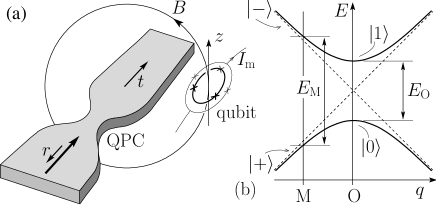
Figure 1: (a) Layout: A (flux) qubit (not to scale, placed downstream the scatterer) is used to measure the fidelity or full counting statistics of a quantum point contact (QPC); the measurement current $I_{\mathrm{m}}$ is switched on only during the readout of the qubit state. For a magnetic coupling $\lambda h\sigma_{z}$, the direction of the magnetic field defines the $z$-axis. (b) Level scheme for the qubit, which is initially prepared in the ground state $|0\rangle$ at the fully frustrated point O and suddenly switched to M at $t=0$ for the measurement, producing an initial state $|\Psi\rangle=[|+\rangle+|-\rangle]/\sqrt{2}$. The semi-classical states $|\pm\rangle$ carry circulating currents perturbing the wire in the measurement of the fidelity; in the measurement of the full counting statistics the state of the qubit is incrementally changed at each passage of a charge through the wire.

In this context, there are two points of view in describing a system (such as a regular or chaotic dot, a quantum wire, etc.) coupled to a qubit: i) the qubit-centered view, where the dot/wire acts as a noisy environment producing decoherence of the qubit state makhlin — this traditional view is pursued in the field of quantum computing; ii) the dot/wire-centered view, where the qubit serves as a measurement device providing information on the system (the dot or wire). This is the new standpoint we take in the present paper where we are interested in two system properties, the fidelity and the full counting statistics.

The notion of fidelity has been introduced in order to quantify the stability of a quantum system (described by the Hamiltonian $H_{\mathrm{sys}}$) under the action of a small external perturbation $\lambda h$ peres : evaluating the evolution of an initial state $\Psi$ under the action of the system’s Hamiltonian $H_{\mathrm{sys}}$, $\Psi(t)=\exp(-iH_{\mathrm{sys}}t/\hbar)\Psi$, comparison is made with the perturbed evolution $\Psi_{\lambda}(t)=\exp[-i(H_{\mathrm{sys}}+\lambda h)t/\hbar]\Psi$ through the matrix element modsq

$$\chi_{\mathrm{fid}}(\lambda,t) = \langle\Psi_{\lambda}(t)|\Psi(t)\rangle$$

$$= \langle\Psi|e^{i(H_{\mathrm{sys}}+\lambda h)t/\hbar}e^{-iH_{\mathrm{sys}}t/\hbar}|\Psi\rangle;$$

a quantum system with a chaotic classical correspondent exhibits a rapid time-decay of the fidelity $\chi_{\mathrm{fid}}$ peres ; jalabert , while a regular classical analogue leads to its saturation at a finite value peres . Above, the fidelity has been defined for a pure state formulated in a first-quantization language; the definition (I) agrees with its quantum information theoretic analogue for two pure state $\Psi$ and $\Psi_{\lambda}$ nielsonchuang .

In general, the interference between two wave functions as manifested in (I) is difficult to measure. Here, we put forward the idea to couple the system under investigation to an external device (e.g., a two-level system in the form of a spin or a qubit) which simultaneously acts as a perturbation and as a measuring device for the fidelity, see Fig. 1(a): the coupling $\lambda h\sigma_{z}$ entangles the system with the measurement device, thus transferring information of the system’s evolution which then can be measured along with the quantum state of the device. A similar idea has been introduced in the context of the full counting statistics (FCS) which is characterizing the charge transport through a quantum wire. The task then is to count the number of transferred charges which corresponds to the measurement of the integrated current $Q(t)=\int_{0}^{t}dt^{\prime}\,I(t^{\prime})$. The straightforward (classical) Ansatz ll1 for the generating function $\chi(\lambda,t)=\langle\exp[i\lambda Q(t)]\rangle$ is problematic as no prescription for the time-ordering of current operators appearing at different instances of time is given. The idea to couple the system to a measurement device resolves these problems: following the work of Levitov and Lesovik ll23 , the complete statistical information can be obtained by coupling the wire to a spin degree of freedom serving as the measuring device; the Fourier coefficients $\int d\lambda\exp(-i\,n\lambda)\chi_{\rm\scriptscriptstyle FCS}(\lambda,t)$ of the generating function

$$\chi_{\rm\scriptscriptstyle FCS}(\lambda,t)=\mathrm{Tr}_{\mathrm{w}}[\rho^{\mathrm{w}}(0)\,e^{i(H_{\mathrm{w}}+\lambda h)t/\hbar}e^{-i(H_{\mathrm{w}}-\lambda h)t/\hbar}]$$ (2)

provide the probabilities $P_{n}(t)$ for the passage of $n$ charges during the time $t$. Here, $H_{\mathrm{w}}$ ($\rho^{\mathrm{w}}(0)$) denotes the wire’s Hamiltonian (density matrix) and $\lambda h$ describes its coupling to the spin; the trace is taken over the wire’s degrees of freedom, while the off-diagonal matrix element has been evaluated in spin space, see below.

II Equivalence between fidelity and FCS

The full counting statistics refers to a many-body system cast in a second-quantized formalism. Still, comparing (I) and (2), we immediately note the similarity of the two expressions: indeed, replacing the arbitrary perturbation in (I) by the coupling to a spin (or two-level system) serving at the same time as a perturbation and as a measurement device, we arrive at the form in (2) with the trace over the wire’s degrees of freedom replaced by the quantum average over the initial state $\Psi$. In previous discussions peres ; jalabert the fidelity of a quantum system has been related to the chaotic/regular nature of the system; probing such a system with a measurement device as described above provides the identical information. The notion of fidelity introduced here generalizes this concept to quantum systems without classical analogue as well as mixed state- and many-particle systems; the quantum information theoretic definition for density matrices nielsonchuang is different, however.

The fidelity/generating function $\chi(\lambda,t)$ is obtained by coupling a spin (in zero external magnetic field) to the system via a Hamiltonian of the form $H_{\mathrm{int}}=\lambda h\sigma_{z}$ (the absence of terms $\propto\sigma_{x,y}$ is crucial). The evolution of the spin then is described by the reduced density matrix

$$\rho^{\mathrm{s}}(t)=\mathrm{Tr}\bigl{[}e^{-i(H_{\mathrm{sys}}+H_{\mathrm{int}})t/\hbar}\rho(0)\,e^{i(H_{\mathrm{sys}}+H_{\mathrm{int}})t/\hbar}\bigr{]}$$ (3)

with the initial separable density matrix $\rho(0)=\rho^{\mathrm{sys}}(0)\otimes\rho^{\mathrm{s}}(0)$ and the trace is taken over the system degrees of freedom without the spin; for the fidelity (I) we have to replace $\rho^{\mathrm{sys}}(0)\to\rho^{\Psi}(0)=|\Psi\rangle\langle\Psi|$. Evaluating the spin part first, we subsequently exploit the cyclic property of the trace and obtain

$$\rho^{\mathrm{s}}_{\sigma_{z}^{\prime},\sigma_{z}}(t)=\rho^{\mathrm{s}}_{\sigma_{z}^{\prime},\sigma_{z}}(0)$$ (4)

$$\qquad\times\mathrm{Tr}\bigl{[}\rho^{\mathrm{sys}}(0)\,e^{i(H_{\mathrm{sys}}+\lambda h\sigma_{z})t/\hbar}e^{-i(H_{\mathrm{sys}}+\lambda h\sigma_{z}^{\prime})t/\hbar}\bigr{]}.$$

The measurement of the off-diagonal entry $\rho^{\mathrm{s}}_{-1,1}(t)$ provides us with the sought-after quantity $\chi(\lambda,t)$.

Below, we will replace the spin degree of freedom by the more versatile qubit. Thereby, we transfer the measurement of the fidelity and of the full counting statistics from the realm of a ‘Gedanken’ experiment to a practical proposal realizable with today’s qubit technology. In this context, we recognize previous steps taken in this direction in measuring the fidelity of a quantum kicked rotator qkr and in the measurement of higher order correlators prober , see also Ref. lesovik_94 for alternative theoretical proposals.

III Measurement with qubits

On a technical level, our problem is described by the Hamiltonian (we formulate the problem for a wire; the extension to other systems is straightforward)

$$H=H_{\mathrm{w}}+H_{\mathrm{q}}+H_{\mathrm{int}}$$ (5)

with $H_{\mathrm{w}}$ the wire’s Hamiltonian of which the fidelity and/or full counting statistics shall be determined,

$$H_{\mathrm{q}}=({\epsilon}/{2})\sigma_{z}-({\Delta}/{2})\sigma_{x}$$ (6)

is the qubit Hamiltonian written in the semi-classical basis $|\pm\rangle$ (see Fig. 1) and

$$H_{\mathrm{int}}=\lambda h\sigma_{z}$$ (7)

is the interaction Hamiltonian coupling the qubit to the wire. For a magnetic (transverse) coupling, we have the standard form

$$H_{\mathrm{int}}=\frac{1}{c}\int_{\mathrm{w}}dxI_{\mathrm{w}}({\bf x})A_{x}({\bf x})\sigma_{z}$$ (8)

with $I_{\mathrm{w}}({\bf x})$ the current flowing in the wire and $A_{x}({\bf x})=\int_{\mathrm{q}}d{\bf l}\cdot\hat{\bf x}\,|I_{\mathrm{q}}|/c|{\bf x}-{\bf l}|$ the gauge potential generated by the qubit current $I_{\mathrm{q}}$; the coupling constant $\lambda$ is defined such as to add a phase $\lambda/2=2\pi\int_{\mathrm{w}}dxA_{x}(x)/\Phi_{0}$ to every electron passing the qubit (here, $\Phi_{0}=hc/e$ denotes the unit of flux). For an electric (longitudinal) coupling pilgrambuttiker , we have the corresponding expression

$$H_{\mathrm{int}}=\int_{\mathrm{w}}dx\rho_{\mathrm{w}}({\bf x})\varphi({\bf x})\sigma_{z}$$ (9)

with $\rho_{\mathrm{w}}({\bf x})$ the 1D charge density of the wire and $\varphi({\bf x})=\int_{\mathrm{q}}d^{2}R\,|\rho_{\mathrm{q}}|/\varepsilon|{\bf x}-{\bf R}|$ the electric potential generated by the qubit charge density $\rho_{\mathrm{q}}({\bf R})$ ($\varepsilon$ is the dielectric constant); again, we choose a splitting into $\lambda$ and $h$ such that each electron passing the qubit acquires an additional phase $\lambda/2=(e/\hbar v)\int_{\mathrm{w}}dx\varphi(x)$ ($e>0$; here, $v$ denotes the (typical) electron velocity and we assume a slowly varying potential, see below for details).

Typical qubits we have in mind are the flux qubit as implemented by Chiorescu et al. chiorescu or the charge qubit built by Vion et al. vion . The generic level diagram for these devices is shown in Fig. 1(b): The semi-classical states $|+\rangle$ and $|-\rangle$ refer to current- (charge-) states which are the energy eigenstates away from the optimally frustrated state. Frustration produces mixing with new eigenstates $|0\rangle=[|+\rangle+|-\rangle]/\sqrt{2}$ and $|1\rangle=[|+\rangle-|-\rangle]/\sqrt{2}$ at the optimal point O where no currents/charges appear on the qubit. In order to measure the fidelity/full counting statistics, the qubit is prepared in the ground state $|0\rangle$ at optimal frustration (point O in Fig. 1(b) with $\Delta=E_{\mathrm{O}}$ and $\epsilon=0$; this corresponds to the spin-state polarized along the $x$-axis) and then is suddenly switched (at time $t=0$) to the measuring point M which has to be chosen sufficiently far away from O to avoid mixing of the semi-classical states (i.e., $\Delta=0$ and $\epsilon=E_{\mathrm{M}}$, hence the Hamiltonian (6) describes a spin in a magnetic field directed along the $z$-axis). On the other hand, the point M should be chosen not too distant away from O in order to avoid the mixing with other levels. At the end of the signal accumulation (i.e., at time $t$) the state of the qubit has to be measured in the following manner: rotation of the qubit state by $-\pi/2$ ($\pi/2$) around the $y$- ($x$-) axis and subsequent measurement along the $z$-axis provides us with the matrix elements $\langle\sigma_{x}\rangle=\mathrm{Tr_{q}}[\rho^{\mathrm{q}}(t)\sigma_{x}]$ ($\langle\sigma_{y}\rangle=\mathrm{Tr_{q}}[\rho^{\mathrm{q}}(t)\sigma_{y}]$) from which the final result $\chi(\lambda,t)=\exp(-iE_{\mathrm{M}}t/\hbar)[\langle\sigma_{x}\rangle+i\langle\sigma_{y}\rangle]$ follows (the phase $\exp(-iE_{\mathrm{M}}t/\hbar)$ compensates the trivial time evolution of the qubit in the finite residual field).

In order to extract the full counting statistics from the generating function $\chi_{\rm\scriptscriptstyle FCS}(\lambda,t)$, a tunable coupling between the wire and the qubit is needed. The tetrahedral superconducting qubit proposed recently feigel lends itself as a particularly useful measurement device: its doubly degenerate ground state emulates a spin in zero magnetic field, hence $H_{\mathrm{q}}=0$, while a symmetric charge bias $\delta^{\scriptscriptstyle Q}$ produces an interaction Hamiltonian $H_{\mathrm{int}}\propto\delta^{\scriptscriptstyle Q}\delta^{\scriptscriptstyle\Phi}\sigma_{z}$ which is linear in the magnetic flux $\delta^{\scriptscriptstyle\Phi}$ (produced by the wire’s current) threading the qubit and easily tunable with $\lambda\propto\delta^{\scriptscriptstyle Q}$ (note that imposing a flux $\delta^{\scriptscriptstyle\Phi}$ the tetrahedral qubit also serves as a tunable charge detector). Alternatively, flux- chiorescu or charge- vion qubits can be used with a flux tunable third junction or an electrically tunable capacitance.

Finally, we have to make sure that the individual electrons passing through the wire are sufficiently coupled to the qubit. This is trivially the case for the electric coupling, where a simple calculation leads to the estimate $\lambda\approx(4e^{2}/\hbar v_{F}\varepsilon)\ln(L/d)$ with $v_{F}$ the Fermi velocity, $L$ the wire’s length, and $d$ its distance from the qubit; with $c/v_{F}\varepsilon$ of order $10^{2}$ or larger a $\lambda$-value beyond unity is easily realized. The situation is less favorable for the case of magnetic coupling: associating the qubit with a magnetic dipole $m_{\mathrm{q}}=I_{\mathrm{q}}S/c$ ($S$ denotes the qubit’s area), we obtain a coupling $\lambda\approx 2\pi\alpha I_{\mathrm{q}}S/ced$, $\alpha=e^{2}/\hbar c$ the finestructure constant. With $I_{\mathrm{q}}$ of order $1~{}\mu$A and $S/d\sim 1~{}\mu$m, we find a coupling $\lambda\sim 10^{-2}$. Similar findings apply to the tetrahedral qubit: applying a homogeneous flux $\delta^{\Phi}$, the qubit can be used as a tunable charge detector with large coupling $\lambda\approx(4E_{J}C/\hbar v_{F})(\delta^{\Phi}/\Phi_{0})\ln(L/d)$, $C$ denoting the capacitive coupling between the wire and the qubit. On the other hand, applying a symmetric charge bias $\delta^{Q}$ we find a magnetic coupling of order $\lambda\approx\alpha(\delta^{Q}/2e)I_{\mathrm{q}}S/2ced$ (we have chosen a typical parameter $E_{J}/E_{C}=10^{2}$). As may be expected, the system is easily coupled to the qubit via electric interaction, while its magnetic coupling is generically weak and has to be suitably enhanced, e.g., with the help of a flux transformer.

The magnetic coupling of the flux qubit allows for the measurement of both the full counting statistics and the system’s fidelity. Going over to the interaction representation (with the unperturbed Hamiltonian given by the system Hamiltonian), the generating function assumes the form (cf. (4))

$$\chi_{\rm\scriptscriptstyle FCS}(\lambda,t)\!=\!\mathrm{Tr}[\rho^{\mathrm{sys}}(0)\,\widetilde{\cal T}e^{i\frac{\lambda}{\hbar}\!\int_{0}^{t}\!dt^{\prime}h(t^{\prime})}\,{\cal T}e^{i\frac{\lambda}{\hbar}\!\int_{0}^{t}\!dt^{\prime}h(t^{\prime})}],$$ (10)

where ${\cal T}$ ($\widetilde{\cal T}$) denote the (reverse) time ordering operators; as desired, the magnetic coupling then is proportional to the integrated current (or transferred charge) $Q(t)=\int_{0}^{t}dt^{\prime}I_{\mathrm{w}}(t^{\prime})$; the form (10) reveals the role of $\chi_{\rm\scriptscriptstyle FCS}(\lambda,t)$ as the generating function for the cumulants of transferred charge. Alternatively, the qubit can be viewed as a system perturbation and $\chi_{\rm\scriptscriptstyle FCS}$ assumes the role of a fidelity $\chi_{\mathrm{fid}}$. The electric coupling to the charge qubit generates a quantity $\chi_{\mathrm{fid}}(\lambda,t)$ whose meaning is predominantly that of a fidelity; on the other hand, for a uniform and unidirectional charge motion with velocity $v_{F}$, the time-integrated charge $\int_{0}^{t}dt^{\prime}\rho_{\mathrm{w}}(t^{\prime})$ can be related to the transferred charge $Q(t)$ via $Q(t)=v_{F}\int_{0}^{t}dt^{\prime}\rho_{\mathrm{w}}(t^{\prime})$ and thus provides an approximate access to the full counting statistics at finite voltage for which the electrons move in a specific direction along the wire.

IV FCS with wave functions

Inspired by the equivalence between the fidelity and the generating function for the counting statistics, we proceed with the calculation of $\chi(\lambda,t)$ within a first-quantized formalism. In particular, we choose a system in the geometry of a point contact and study the fidelity for the case where a wave packet is incident on the scatterer. This scheme allows for a more elaborate discussion of the various parametric dependencies of the fidelity/FCS but suffers from the restriction to a single particle. In order to ameliorate this limitation, we extend the discussion to a sequence of two incident wave packets, from which the extrapolation to the many body case can be performed.

Consider a wave packet (for $t\to-\infty$ and traveling to the right)

$$\Psi_{\mathrm{in}}(x,t)\equiv\Psi_{f}(x,t)=\int\frac{dk}{2\pi}\,f(k)\,e^{i(kx-\omega_{k}t)},$$ (11)

centered around $k_{0}>0$ with $\omega_{k}=\hbar k^{2}/2m$ and normalization $\int(dk/2\pi)|f(k)|^{2}=1$, incident on a scatterer characterized by transmission and reflection amplitudes $t_{k}$ and $r_{k}$. We place the qubit behind the scatterer to have it interact with the transmitted part of the wave function. The transmitted wave packet then acquires an additional phase due to the interaction with the qubit: for a magnetic interaction the extra phase accumulated up to the position $x$ amounts to $\delta\phi_{A}(x)=2\pi\int^{x}dx^{\prime}\,A_{x}(x^{\prime})/\Phi_{0}$, independent of $k$; as $x\to\infty$ this adds up to a total phase $\lambda/2=2\pi\int_{-\infty}^{\infty}dx\,A_{x}(x)/\Phi_{0}$, cf. (8). For an electric interaction, cf. (9), the situation is slightly more involved: the extra phase can be easily determined for a slowly varying (quasi-classical) potential of small magnitude, i.e., $e|\varphi|\ll\hbar^{2}k_{0}^{2}/2m$. Expanding the quasi-classical phase $\int^{x}dx^{\prime}\,p(x^{\prime})/\hbar$ with $p(x)=\sqrt{2m(E+e\varphi(x))}$ to first order in the potential $\varphi(x)$ yields the phase $\delta\phi_{\varphi}(x)=(e/\hbar v)\int^{x}dx^{\prime}\,\varphi(x^{\prime})$ which asymptotically accumulates to the value $\lambda/2$; its $v$-dependence is due to the particle’s acceleration in the scalar potential and will be discussed in more detail below. Moreover, note that $\phi_{A}$ changes sign for a particle moving in the opposite direction ($k\to-k$) (i.e., under time reversal) whereas $\phi_{\varphi}$ does not. For a qubit placed behind the scatterer both magnetic and electric couplings produce equivalent phase shifts. Depending on the state $|\pm\rangle$ of the qubit, the outgoing wave (for $t\to\infty$)

$$\Psi_{\mathrm{out}}^{\pm}(x,t)=\int\frac{dk}{2\pi}f(k)e^{-i\,\omega_{k}t}\bigl{[}r_{k}e^{-ikx}\Theta(-x)$$

$$\qquad\qquad\qquad\qquad\qquad+e^{\pm i\lambda/2}t_{k}e^{i\,kx}\Theta(x)\bigr{]}$$

acquires a different asymptotic phase on its transmitted part. The fidelity is given by the overlap of the two outgoing waves,

$$\chi(\lambda,t)=\int dx{\Psi_{\mathrm{out}}^{-}}^{*}(x,t)\Psi_{\mathrm{out}}^{+}(x,t)$$ (12)

$$\qquad=\int\frac{dk}{2\pi}(R_{k}+e^{i\lambda}T_{k})|f(k)|^{2}\equiv\langle R\rangle_{f}+e^{i\lambda}\langle T\rangle_{f},$$

where $R_{k}=|r_{k}|^{2}$ and $T_{k}=|t_{k}|^{2}$ denote the probabilities for reflection and transmission, respectively, and we have neglected exponentially small off-diagonal terms involving products $\int dkf(-k)^{*}f(k)$. The result (12) applies to both magnetic and electric couplings; its interpretation as the generating function of the charge counting statistics provides us with the two non-zero Fourier coefficients $P_{0}=\langle R\rangle_{f}$ and $P_{1}=\langle T\rangle_{f}$ which are simply the probabilities for reflection and transmission of the particle. This result agrees with the usual notion of ‘counting’ those particles which have passed the qubit behind the scatterer. When, instead, the interest is in the system’s sensitivity, we observe that the fidelity $\chi(\lambda,t)$ lies on the unit circle only for the ‘trivial’ cases of zero or full transmission $T=0,~{}1$, i.e., in the absence of partitioning, or for $\lambda=2\pi\mathbb{Z}$; the latter condition corresponds to no counting or the periodic vanishing of decoherence in the qubit. On the contrary, in the case of maximal partitioning with $\langle R\rangle_{f}=\langle T\rangle_{f}=1/2$, a simple phase shift by $\lambda=\pi$ makes the fidelity vanish altogether. Hence, partitioning has to be considered as a (purely quantum) source of sensitivity towards small changes, as chaoticity generates sensitivity in a quantum system with a classical analogue.

The result (12) also applies for a qubit placed in front of the scattering region provided the coupling is of magnetic nature (for the reflected wave, the additional phases picked up in the interaction region cancel, while the phase in the transmitted part remains uncompensated). However, an electric coupling behaves differently under time reversal and the fidelity acquires the new form

$$\chi(\lambda,t)=e^{i\lambda}\bigl{(}e^{i\lambda}\langle R\rangle_{f}+\langle T\rangle_{f}\bigr{)}.$$ (13)

Next, we comment on the (velocity) dispersion in the electric coupling $\lambda$: the different components in the wave packet then acquire different phases. To make this point more explicit consider a Gaussian wave packet centered around $k_{0}$ with a small spreading $\delta k\ll k_{0}$ and denote with $\lambda_{0}$ the phase associated with the $k_{0}$ mode. The spreading $\delta k$ in $k$ generates a corresponding spreading in $\delta\lambda\approx\lambda_{0}(\delta k/k_{0})$ which leads to a reduced fidelity

$$\chi(\lambda,t)=\langle R\rangle_{f}+\langle e^{i\lambda}T\rangle_{f}\approx R_{k_{0}}+e^{i\lambda_{0}-\frac{\lambda_{0}^{2}(\delta k)^{2}}{2k_{0}^{2}}}T_{k_{0}},$$ (14)

where we have assumed a smooth dependence of $T_{k}$ over $\delta k$ in the last equation. The reduced fidelity for $T=1$ is due to the acceleration and deceleration produced by the two states of the qubit ac . The wave packets passing the qubit then acquire a different time delay depending on the qubit’s state. As a result, the wave packets become separated in space with an exponentially small residual overlap for the Gaussian shaped packets.

Next, we consider the case with two wave packets incident on the scatterer, $\Psi_{\mathrm{in}}\propto[\Psi_{f_{1}}(x_{1})\Psi_{f_{2}}(x_{2})\pm(x_{1}\leftrightarrow x_{2})]\chi_{s/t}(s_{1},s_{2})$, where $f_{1,2}$ denote different wave packet amplitudes, cf. (11), and $\chi_{s/t}$ are the singlet/triplet spin functions. Placing the qubit behind the scatterer, we obtain the fidelity

$$\!\!\chi_{2}(\lambda,t)=\frac{1}{N_{\pm}}\Bigl{[}{\prod_{m=1,2}}\int\!\frac{dk_{m}}{2\pi}|f_{m}(k_{m})|^{2}(R_{k_{m}}+e^{i\lambda}T_{k_{m}})$$

$$\pm\!{\prod_{m=1,2}}\int\!\frac{dk_{m}}{2\pi}f^{*}_{m}(k_{m})f_{n\neq m}(k_{m})(R_{k_{m}}+e^{i\lambda}T_{k_{m}})\Bigr{]},$$ (15)

with the normalization $N_{\pm}=1\pm|S|^{2}$, $S=\int(dk/2\pi)$ $f^{*}_{1}(k)f_{2}(k)$, and we have made use of the fact that all components of the wave packet propagate in specific directions such that $\int dkf^{*}_{n}(k)f_{m}(-k)=0$. The fidelity (15) involves two terms, a direct term independent of the spin/orbital symmetry and an exchange term that can be neglected if the two wave packets are well separated either in momentum space (with $k_{0n}$ sufficiently different) or in real space (with $k_{0}\delta x\gg 1$). In both of these cases the overlap $S$ vanishes and we arrive at the final result

$$\chi_{2}(\lambda,t)=[\langle R\rangle_{f_{1}}+e^{i\lambda}\langle T\rangle_{f_{1}}][\langle R\rangle_{f_{2}}+e^{i\lambda}\langle T\rangle_{f_{2}}],$$ (16)

i.e., the fidelity of the two-particle system is just the product of the single particle fidelities. The result can be trivially generalized to the many particle case provided that exchange terms can be neglected, as is the case for a sequence of ($N$) properly separated wave packets. The result $\chi_{N}(\lambda,t)=\Pi_{n=1}^{N}[\langle R\rangle_{f_{n}}+e^{i\lambda}\langle T\rangle_{f_{n}}]$ then has to be compared with the previous finding $\chi_{V}(\lambda,t)=[R+e^{i\lambda}T]^{e|V|t/h}$ lc ; ll23 calculated at constant voltage $V$ within a many-body formalism. The validity of the latter result is restricted to non-dispersive scattering coefficients $T$ and $R$. Identifying $e|V|t/h$ with the number $N$ of transmitted particles the two results agree. However, we note that the present derivation corresponds to a voltage driven many-body setup where distinct voltage pulses with unit flux $c\int dt\,|V(t)|=\Phi_{0}$, each transferring one particle, are applied to the system ll23 . The detailed comparison of these two cases, pulsed versus constant voltage, and the absence of interference terms in the latter case is an interesting problem for further investigation. The extension of the fidelity to the many-body case puts additional emphasis on the relation between sensitivity and partitioning (see also Ref. agam_00 ) as any finite partitioning with $T<1$ now generates a fidelity which is vanishing exponentially in time; the quantity $-\ln[1-4RT\sin^{2}(\lambda/2)]/\Delta t$ with $\Delta t$ the time separation between two wave packets/voltage pulses then plays the role of the Lyapunov exponent in systems with a classical chaotic correspondent.

In summary, we have unified the themes of fidelity and full counting statistics and have shown how to exploit qubits for their measurement. As an application of these ideas, we have recalculated the generating function for the full counting statistics within a wave packet approach. This allows for a more in-depth analysis of the counting problem and helps to shed light on the ongoing discussion lc relating different expressions for high-order correlators to variations in the experimental setup.

We thank Lev Ioffe for discussions and acknowledge financial support by the CTS-ETHZ, the MaNEP program of the Swiss National Foundation and the Russian Science Support Foundation.

References

- (1) A. Peres, Phys. Rev. A 30, 1610 (1984).
- (2) L.S. Levitov and G.B. Lesovik, JETP Lett. 58, 230 (1993) and cond-mat/9401004 (1994); L.S. Levitov, H. Lee, and G.B. Lesovik, J. Math. Phys. 37, 4845 (1996).
- (3) M.A. Nielsen and I.L. Chuang, Quantum Computation and Quantum Information (Cambridge University Press, Cambridge, 2000).
- (4) I. Chiorescu, Y. Nakamura, C.P.M. Harmans, and J.E. Mooij, Science 299, 1869 (2003).
- (5) D. Vion, A. Aassime, A. Cottet, P. Joyez, H. Pothier, C. Urbina, D. Esteve, and M. Devoret, Science 296, 886 (2002).
- (6) Y. Makhlin, G. Schön, and A. Shnirman, Rev. Mod. Phys. 73, 357 (2001).
- (7) D.V. Averin and E.V. Sukhorukov, Phys. Rev. Lett. 95, 126803 (2005).
- (8) R. Aguado and L.P. Kouwenhoven, Phys. Rev. Lett. 84, 1986 (2000); R.J. Schoelkopf, A.A. Clerk, S.M. Girvin, K.W. Lehnert, and M.H. Devoret, in Quantum Noise in Mesoscopic Physics, ed. Y. Nazarov (Kluver, Amsterdam, 2003).
- (9) The usual definition peres involves the square modulus of this quantity.
- (10) R.A. Jalabert and H.M. Pastawski, Phys. Rev. Lett. 86, 2490 (2001).
- (11) L.S. Levitov and G.B. Lesovik, JETP Lett. 55, 555 (1992).
- (12) S.A. Gardiner, J.I. Cirac, and P. Zoller, Phys. Rev. Lett. 80, 2968 (1998); S. Montangero, A. Romito, G. Benenti, and R. Fazio, Europhys. Lett. 71, 893 (2005).
- (13) B. Reulet, J. Senzier, and D.E. Prober, Phys. Rev. Lett. 91, 196601 (2003); R.K. Lindell, J. Delahaye, M.A. Sillanpaa, T.T. Heikkila, E.B. Sonin, and P.J. Hakonen, Phys. Rev. Lett. 93, 197002 (2004); Yu. Bomze, G. Gershon, D. Shovkun, L.S. Levitov, and M. Reznikov, cond-mat/0504382.
- (14) G.B. Lesovik, JETP. Lett. 60, 820 (1994); J.P. Pekola, Phys. Rev. Lett. 93, 206601 (2004); E.B. Sonin, Phys. Rev. B 70, 140506(R) (2004) and cond-mat/0505424.
- (15) S. Pilgram and M. Büttiker, Phys. Rev. B 67, 235308 (2003).
- (16) M.V. Feigel’man, L.B. Ioffe, V.B. Geshkenbein, P. Dayal, and G. Blatter, Phys. Rev. Lett. 92, 098301 (2004).
- (17) The fidelity involves the matrix element of wave functions perturbed by opposite states of the qubit.
- (18) G.B. Lesovik and N.M. Chtchelkatchev, JETP Lett. 77, 393 (2003).
- (19) O. Agam, I. Aleiner, and A. Larkin, Phys. Rev. Lett. 85, 3153 (2000).