On The Universal Scaling Relations In Food Webs

Abstract

In the last three decades, researchers have tried to establish universal patterns about the structure of food webs. Recently was proposed that the exponent $\eta$ characterizing the efficiency of the energy transportation of the food web had a universal value ($\eta=1.13$). Here we establish a lower bound and an upper one for this exponent in a general spanning tree with the number of trophic species and the trophic levels fixed. When the number of species is large the lower and upper bounds are equal to $1$, implying that the result $\eta=1.13$ is due to finite size effects. We also evaluate analytically and numerically the exponent $\eta$ for hierarchical and random networks. In all cases the exponent $\eta$ depends on the number of trophic species $K$ and when $K$ is large we have that $\eta\to 1$. Moreover, this result holds for any number $M$ of trophic levels. This means that food webs are very efficient resource transportation systems.

Understanding energy and material fluxes through ecosystems is central to many questions in ecology 1 ; 2 ; 3 . Ecological communities can be studied via resource transfer in food webs 4 . These webs are diagrams showing the predation relationships among species in a community. Usually, a group of species sharing the same set of predators and the same set of prey is aggregated in one trophic specie 5 ; 6 . So, each trophic specie is represented by a site and denoted by an integer number $i=1,...~{},K$, where $K$ is the total number of trophic species. A relation between a pair of sites is represented by a link directed from the prey to predator. There are several quantities introduced in the literature to characterize the food web structure, such as the fractions of the species in the trophic levels (basal, intermediates and top), the fractions of links among them, the connectance, the average distance between two sites, the clustering coefficient and the degree distribution. It turns out that all these quantities are nonuniversal Garla2 and dependent of the size of the food web. Perhaps, the only variable in common agreement with the literature is the maximum value of trophic levels $(M\leq 4)$. Garlaschelli et al. Garla1 have considered food web as transportation networks banavar ; west whose function is to deliver resources from the environment to every specie in the network. In this case, food webs appear to be very similar to other systems with analogous function, such as river and vascular networks. In that work they have represented a real food web by spanning trees with minimal lengths. For each specie $i$ the number $A_{i}$ of species feeding directly or indirectly on $i$, plus itself, is computed. They also computed the cost of this transfer, namely $C_{i}=\sum_{k}A_{k}$, where $k$ runs over the set of direct an indirect predators of $i$ plus itself. The shape of $C_{i}$ as a function of $A_{i}$ follows a power law relation $C\left(A\right)\sim A^{\eta}$, where the scaling exponent $\eta$ quantifies the degree of optimization of the transportation network. They found the same allometric scaling relation for different food webs. By plotting $C_{i}$ versus $A_{i}$ for each one of the seven large food webs in the literature, and by plotting $C_{0}$ versus $A_{0}$ for a set of different food webs. The exponent found, varies between $1.13$ and $1.16$. Therefore, they concluded that the exponent $\eta$ has a universal value ($\eta=1.13$) and it is, perhaps, the only universal quantity in food webs. Nevertheless, this matter has been the subject of debates camacho ; Garla3 .

Here we establish an upper bound ($\eta_{max}$) and a lower one ($\eta_{min}$) for the exponent $\eta$ in a general spanning tree with $M$ trophic levels and $K$ trophic species, both fixed. In the limit $K\to\infty$, we have that $\eta_{max}=\eta_{min}\to 1$. We also evaluate analytically and numerically the exponent $\eta$ for hierarchical and random networks. Our main conclusions are that (a) the result $\eta=1.13$ for food webs is due to finite size effect (small $K$), (b) the exponent $\eta$ depends on the $K$ and when $K$ is large we have that $\eta=1$. Moreover, this results hold for any number $M$ of trophic levels, implying that food webs are efficient resource transportation networks.

It is worth mentioning that this problem is related to river and vascular networks banavar . Consider $K$ sites uniformly distributed in a $d$-dimensional volume. The network is constructed by linking the sites, in such way that there is at least a path connecting each site to the source (a central site). Since each site is feed at steady rate $F_{i}=F$,the metabolic rate $B$ clearly is given by $B=\sum_{i}F_{i}=FK$. Let $I_{b}$ represent the magnitude of flow on the $b^{th}$ link. Then, the total quantity of nutrients in the network, at a particular time, is given by $V=\sum_{b}I_{b}$. They define the most efficient class of network as that for which $V$ is small as possible. Using this procedure they found that $V\sim B^{(d+1/d)}$. For river basins, $d=2$ and $V\sim B^{3/2}$. In vascular systems $V\sim B^{4/3}$ since $d=3$. The variables $A_{0}$ and $C_{0}$ of the food webs are related, respectively, to the number of transfer sites $N$ and to the total volume of nutrients $V$ by the following equations: $N=A_{0}-1$ and $V=C_{0}-A_{0}$. Then we have that $C_{0}\approx A_{0}^{(d+1/d)}$ if $A_{0}$ is large enough. The value of the exponent $\eta$ for a food web can be smaller than the one of rivers ($\eta=3/2$) or the one of vascular systems ($\eta=4/3$) because the spanning tree of a food web is not embedded in an Euclidean space.

Let us consider a hierarchical network with $M$ trophic levels. The network is constructed in the following way. We begin with a site representing the environment, the site $0$. Then we connect $n_{1}$ sites to it, since these sites are feeding directly of the environment they constitute the first trophic level. Obviously, the number of species in this level is $N_{1}=n_{1}$. The second level is constructed by connecting $n_{2}$ sites to each site of the first level. Now, in this level, we have $N_{2}=n_{1}n_{2}$ species. This procedure is repeated until the level $M$.

Since $A_{i}$ is the number of species feeding directly or indirectly on site $i$, plus itself, we have that

$$A_{M} = 1$$

$$A_{M-1} = n_{M}A_{M}+1=n_{M}+1$$

$$A_{M-2} = n_{M-1}A_{M-1}+1=n_{M}n_{M-1}+n_{M-1}+1$$

$$\vdots$$

$$A_{0} = 1+\sum^{M}_{\alpha=1}N_{\alpha}=K+1~{}~{}.$$

The cost of resource transfer, defined by $C_{i}=\sum_{k}A_{k}$, where $k$ runs over the set of direct and indirect predators of $i$ plus itself is given by

$$C_{M} = 1$$

$$C_{M-1} = n_{M}C_{M}+A_{M-1}=2n_{M}+1$$

$$C_{M-2} = n_{M-1}C_{M-1}+A_{M-2}=3n_{M}n_{M-1}+2n_{M-1}+1$$

$$\vdots$$

$$C_{0} = 1+\sum^{M}_{\alpha=1}(\alpha+1)\prod^{\alpha}_{i=1}n_{i}=1+\sum^{M}_{\beta=1}(1+\beta)N_{\beta}~{}~{}.$$

The exponent $\eta$, as was proposed in the literature Garla1 , can be found by (a) plotting $C_{i}$ as a function of $A_{i}$ for a network with number of trophic level $M$ and total specie number $K$ fixed; Usually, the point $(1,1)$ is neglected due to finite size effects. It can be also found by (b) plotting $C_{0}$ as a function of $A_{0}$ for several networks with different trophic species number $K$. This last procedure determines the large scale exponent Garla3 . Note that in hierarchical spanning tree networks, $C_{i}$ and $A_{i}$ for species in the same trophic level are equal, implying that we have only $M+1$ points in a $C_{i}\times A_{i}$ plot. Let us firstly use procedure (a) for networks with constant ramification ratio $n_{i}=n$ and constant number of trophic levels $M=4$. We find $\eta=1.39$ for $n=2$ and $K=30$ and $\eta=1.27$ for $n=3$ and $K=120$, as it is shown in figure  1. Clearly, the exponent $\eta$ depends on value of $K$, and decreases as long as $K$ grows. In the limit that $n\to\infty$, the total number of species $K$ also is unlimited and we obtain that the exponent $\eta$ approaches the value $1$.

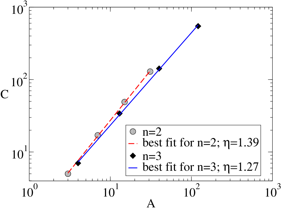
Figure 1: Log-log plots of $C_{i}$ versus $A_{i}$ for networks with constant ramification ratio $n=2$ and $n=3$. Note that the exponent decreases when $n$ grows.

Let us return to the more general case of hierarchical models. The large scale exponent $\eta$ can be evaluated by,

$$\eta=\frac{\ln C_{0}}{\ln A_{0}}=\frac{\ln[1+\sum_{\alpha=1}^{M}(\alpha+1)\prod_{i=1}^{\alpha}n_{i}]}{\ln(1+\sum^{M}_{\alpha=1}\prod_{i=1}^{\alpha}n_{i})}~{}~{}.$$ (1)

If at least a ramification ratio is large, $n_{\beta}\to\infty$, we have that $\ln A_{0}\approx\ln n_{\beta}$ and $\ln C_{0}\approx\ln n_{\beta}$. Therefore we find $\eta\to 1$ when the number of species is large. We can also use Eq. 1 to evaluate the exponent $\eta$ for hierarchical networks with constant ramification ration. We find for this networks $\eta=1.41$ ($n=2$ and $K=30$) and $\eta=1.31$ ($n=3$ and $K=120$). These values can be compared with the ones obtained previously with procedure (a) (see Fig. 1).

In the Eq. 1 the exponent $\eta$ depends on value of $K$, decreasing as long as $K$ grows. For example, consider the hypothetical food web with total specie trophic number $K=146$ and the specie trophic numbers in each level given by $N_{1}=38$, $N_{2}=63$, $N_{3}=43$ and $N_{4}=2$. We find the exponent $\eta=1.22$. But, if we double the number of trophic species in each trophic level $N_{i}=2N_{i}$ the exponent is now $\eta\approx 1.19$. In that equation the exponent $\eta$ also depends in the relative distribution of the species in each level, for a given total specie number $K$. For the hypothetical food web described above with $146$ trophic species we change the distributions of species in each level to $N_{1}=114$, $N_{2}=20$, $N_{3}=10$ and $N_{4}=2$. We find the exponent $\eta=1.16$. The exponent has changed from $\eta=1.22$ to $\eta=1.16$

Now, let us consider a random network with $M$ trophic levels and $K$ trophic species. The network is constructed in the following way. First, we determine randomly the population in each level $N_{\alpha}$ ($\alpha=1,~{}2,\ldots,~{}M$), obeying the restrictions $M$ fixed and $K$ fixed. Then, the $N_{1}$ sites are connected to the environment, constituting the first trophic level. The second level is constructed by randomly connecting the $N_{2}$ sites to the $N_{1}$ sites of the first level. This procedure is repeated until the level $M$ is constructed. In this case, we can evaluate the mean value of $A_{i}$ and $C_{i}$ in each level, namely

$$\overline{A}_{\alpha}=\frac{1}{N_{\alpha}}\sum_{j\in\alpha}A_{j}$$

$$\overline{C}_{\alpha}=\frac{1}{N_{\alpha}}\sum_{j\in\alpha}C_{j}~{}~{}.$$

Here $\alpha$ specify the trophic level ($\alpha=1,\ldots,~{}M$). These quantities are averaged on several random configurations. Note that in the last level we have that $\overline{A}_{M}=A_{i}=C_{i}=\overline{C}_{M}=1$ and that we always neglect the point $(1,1)$ in all fits

In Fig. 2(a) it is shown the $\overline{C}_{\alpha}\times\overline{A}_{\alpha}$ graph for a random network with $K=123$, the same number of trophic specie that the Ythan Estuary with parasites, and $M=4$. A best fit furnishes $\eta=1.18$. A similar fit for $K=93$, the same number of trophic specie that the Little Rock Lake food web, and $M=4$ give us $\eta=1.21$. Note that the exponent decrease when $K$ increases. Clearly, our exponent is larger than that found by  Garla1 for the same trophic species number $K$. But, when $K$ grows our exponent become smaller that them. Obviously, if $\eta=1.13$ represent a universal value for food webs of all the sizes, then random spanning trees networks with the same number of trophic levels $M$ are more efficient than food webs. In fig. 2(b) it is shown the $\overline{C}_{\alpha}\times\overline{A}_{\alpha}$ graph for a random network with $K=10000$ and $M=4$. Note that when $K$ is large enough the exponent $\eta\approx 1$

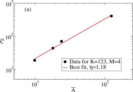
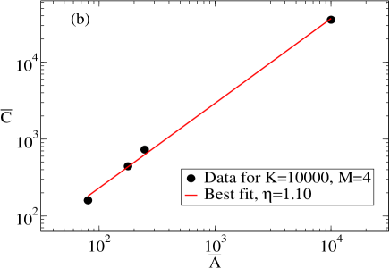
Figure 2: Log-log Plots for random networks. (a) $\overline{C}_{\alpha}\times\overline{A}_{\alpha}$ for a network with $K=123$ and $M=4$ (b)$\overline{C}_{\alpha}\times\overline{A}_{\alpha}$ graph for a random network with $K=10000$ and $M=4$. Note that when $K$ is large enough the exponent $\eta\approx 1$

The exponent $\eta$ can also be computed by the procedure (b). For each value of $K$ we perform an average for several configurations and find the mean value of $C_{0}$. In Fig. 3(a), it is shown the $C_{0}\times A_{0}$ plot for random networks with $M=4$ and $K$ varying from $50$ up to $1000$. Now we have that $\eta=1.00$. It is worth mentioning, that $C_{0}\times A_{0}$ always furnishes $\eta=1$ independently of the range of $K$. We have also simulated random networks with $M=10$ trophic levels. In Fig. 3(b) it is shown the $C_{0}\times A_{0}$ plot. The results are similar.

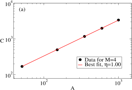
Figure 3: Log-log Plots for random networks. (a) $C_{0}\times A_{0}$ for $M=4$ and $K$ varying from $50$ up to $1000$ and (b) $C_{0}\times A_{0}$ for $M=10$ and $K$ varying from $200$ up to $5000$. Note that the large scale exponent has the same value $\eta=1.00$ and is independent of $M$.

Now let us present the central point of this paper, a general argument to demonstrate that the large scale exponent is $\eta=1$ for large $K$. Let us consider a spanning tree with $M$ and $K$, both fixed. To obey the constraint of $M$ fixed, we put one site in each level. Now we must put each one of the reminder $K-M$ sites. Since $C_{0}$ is cumulative, a site put as near as possible of the environment has the minimal contribution to the global cost. On the other hand, a site put as far as possible of the environment has a maximal contribution to $C_{0}$. To construct the network with maximum value of $C_{0}$, $C_{0,max}$, we must link all $K-M$ sites to the site of the last level. In this network we have $N_{1}=N_{2}=\dots=N_{M-1}=1$ and $N_{M}=K-M+1$. $C_{0,min}$ is obtained by linking the $K-M$ sites directly to the site representing the environment. In this case, we have that $N_{1}=K-M+1$ and $N_{2}=N_{3}=\dots=N_{M}=1$. Note that these constructions are the closest networks to the star-like and chain-like ones, respectively, that obey the constraints of $M$ and $K$ fixed. Using the Eq. 1 we have,

$$C_{0,min} = 1+2K+\frac{M}{2}(M-1)$$

$$C_{0,max} = 1+K(M+1)+\frac{M}{2}(1-M)$$

Then, the lower and the upper bounds for the exponent $\eta$ are

$$\eta_{max} = \frac{\ln C_{0,max}}{\ln(K+1)}=\frac{\ln[1+K(M+1)+\frac{M}{2}(1-M)]}{\ln(K+1)}~{}~{},$$

$$\eta_{min} = \frac{\ln C_{0,min}}{\ln(K+1)}=\frac{\ln[1+2K+\frac{M}{2}(M-1)]}{\ln(K+1)}~{}~{}.$$

When $K\to\infty$, we have that $\eta_{max}=\eta_{min}\to 1$.

Consider again the simulation of random networks. We verified that the constructions with minimum and maximum $C_{0}$ are the ones just described. Moreover, the result above explains why we find $\eta\to 1$ when $K$ is large in the simulations of random networks.

In summary, we studied the transportation properties of several networks that represent spanning trees of food webs. First, we analyzing an idealized hierarchical model that can be analytically solved. Then we show that the exponent $\eta$ depends on value of $K$ and, in the limit that $K$ is large enough, the exponent $\eta$ approaches the value $1$. After, we construct random networks that more realistically represents a spanning tree formed by food webs. We evaluate numerically the exponent $\eta$ by several procedures. Again, in all cases the exponent depends on size of web and if $K$ is large $\eta\to 1$. One important point is that all the results are independent of the number of trophic levels $M$. Moreover, we establish a maximum and a minimum values for the exponent $\eta$ in a general spanning tree with $K$ and $M$ fixed. When the number of species is large these values became equal to $1$. Therefore, we must find $\eta=1$ for a large food web and we can conclude that food webs are very efficient resource transportation systems.

The authors thank to Fundação de Amparo à Pesquisa do Estado de Minas Gerais (FAPEMIG), Coordenação de Aperfeiçoamento de Pessoal de Nível Superior (CAPES) and to Conselho Nacional de Pesquisa (CNPq), Brazilian agencies.
^‡ Electronic address: lbarbosa@fisica.ufmg.br
^∗ Electronic address: alcides@fisica.ufmg.br
^† Electronic address: jaff@fisica.ufmg.br

References

- (1) J. H. Lawton in Ecological Concepts, 43-78, eds. J. M. Cherret, Blackwell Scientific, Oxford (1989).
- (2) S. L. Pimm, Food Webs, Chapman & Hall, London (1982).
- (3) J. E. Cohen, F. Briand and C. M. Newman, Community Food Webs: Data and Theory , Biomathematics 20, Springer, Berlin (1990).
- (4) C. S. Elton, Animal Ecology, Sidgwick and Jackson , London (1927).
- (5) N. D. Marinez, Ecol. Monogr. 61, 367 (1991).
- (6) R. J. Williams and N. D. Marinez, Nature 404, 180 (2000).
- (7) D. Garlaschelli, Eur. Phys. J. B. 38, 277 (2004).
- (8) D. Garlaschelli, G. Caldarelli & L. Pietronero, Nature 423, 165 (2003).
- (9) J. R. Banavar, A. Maritan & A. Rinaldo, Nature 399, 130 (1999).
- (10) G. B. West, J. H. Brown, B. J. Enquist, Science 276, 122 (1997).
- (11) J. Camacho, A. Arenas, Nature 435, doi:10.1038/nature03839 (2005)
- (12) D. Garlaschelli, G. Caldarelli & L. Pietronero, Nature 435,(7044): E4-E4 JUN 16 (2005)