Conductance of quantum wires: a numerical study of the effects of an impurity and interactions

Abstract

We use the non-equilibrium Green’s function formalism and a self-consistent Hartree-Fock approximation to numerically study the effects of a single impurity and interactions between the electrons (with and without spin) on the conductance of a quantum wire. We study how the conductance varies with the wire length, the temperature, and the strengths of the impurity and interactions. The numerical results for the dependence of the conductance on the wire length and temperature are compared with the results obtained from a renormalization group analysis based on the Hartree-Fock approximation. For the spin-1/2 model with a repulsive on-site interaction or the spinless model with an attractive nearest neighbor interaction, we find that the conductance increases with increasing wire length or decreasing temperature. This can be explained using the Born approximation in scattering theory. For a strong impurity, the conductance is significantly different for a repulsive and an attractive impurity; this is due to the existence of a bound state in the latter case. In general, the large density deviations close to the impurity have an appreciable effect on the conductance at short distances which is not captured by the renormalization group equations.

]

I Introduction

The conductance of electrons in a quantum wire has been the subject of intensive study in recent years, both experimentally [2, 3, 4, 5, 6, 7] and theoretically [8, 9, 10]. For a wire in which only one channel is available to the electrons and the transport is ballistic (i.e., there are no impurities inside the wire, and there is no scattering from phonons or from the contacts between the wire and its two leads), the conductance is given by $G=2e^{2}/h$ for infinitesimal bias [11, 12]. This result is expected to hold even if one takes into account the interactions between the electrons since such two-body scatterings conserve the momentum. However, if there is an impurity inside the wire which scatters the electrons, then the conductance is reduced because such a scattering does not conserve the momentum of the electron. For a one-dimensional system containing a $\delta$-function impurity with strength $V$, we obtain

$$G~{}=~{}\frac{2e^{2}}{h}~{}(1~{}-~{}c~{}V^{2}~{})~{},$$ (1)

to lowest order in $V$, where $c$ is a constant related to the Fermi velocity of the electrons (see the discussion below Eq. (4)). (The situation is different if the wire is only quasi-one-dimensional, and the impurity potential has a finite range [13]). In the absence of interactions, $G$ does not depend on the wire length $L$ or the temperature $T$ (as long as $k_{B}T$ is much less than the Fermi energy). But in the presence of interactions, it turns out that $V$ effectively becomes a function of the length scale (which is related to either $L$ or $T$ as will be explained below), and $G$ therefore varies with $L$ and $T$. The variation of $V$ with length scale is governed by a renormalization group (RG) equation. (In this paper, we will only consider a non-magnetic impurity which scatters electrons in a spin independent way).

There are three length scales which are of interest in the problem. The smallest of them is $\lambda\equiv\pi/k_{F}$ (where $k_{F}$ is the Fermi wavenumber); this is the wavelength of the oscillations in the electronic density near impurities as we will see. The other two length scales are the length of the wire $L$, and the thermal coherence length $L_{T}$ which is equal to $\hbar v_{F}/(k_{B}T)$ (where $v_{F}$ is the Fermi velocity). $L_{T}$ gives an idea of the distance beyond which an electron wave function loses its phase coherence. At a temperature $T$, the conductance typically receives contributions from a number of states near the Fermi energy whose energies have a spread of the order of $\Delta E=k_{B}T$. Hence the spread in momentum $\Delta p=\Delta E/v_{F}$ is of the order of $k_{B}T/v_{F}$. A superposition of waves with such a spread of momenta loses phase coherence in a distance of the order of $L_{T}=\hbar v_{F}/(k_{B}T)$. Electronic transport is therefore thermally incoherent if the wire length $L>>L_{T}$, coherent if $L<<L_{T}$, and partially coherent in the intermediate range. This will become clearer when we discuss our numerical results.

The RG equations for the transmission coefficient $|t|^{2}$ has been derived from continuum theories in several ways [8, 9, 14, 15, 16]. We will discuss these equations for two models in Sec. II. (The conductance is related to the transmission as $G=(2e^{2}/h)|t|^{2}$, where the factor of 2 is due to the electron spin). The RG equation is used to analytically follow the evolution of $|t|^{2}$ starting from a short distance scale and going up to a length scale which is the smaller of the two quantities $L$ and $L_{T}$. If $L>>L_{T}$, the conductance is governed by $L_{T}$ and not $L$, and vice versa if $L_{T}>>L$. The RG equation has two fixed points which lie at $|t|^{2}=0$ and 1; the system approaches one of these fixed points if $L$ and $L_{T}$ are both very large.

The above statements are only valid for length scales much longer than $\lambda$ because only then can one use a continuum description from which the RG equation is derived. It would therefore be useful to consider an alternative method for computing the conductance which works even at short length scales where the continuum description is not valid. An interesting thing which occurs at short distances is that if the impurity provides an attractive potential to the electrons, there is a bound state whose wave function decays exponentially away from the impurity. We may wonder what effect a bound state has on the conductance; the RG equations mentioned above do not take this state into account. One may think that a bound state (whose energy lies outside the bandwidth of the leads) cannot directly affect the conductance, because electrons coming in from or going out to the leads cannot enter or leave such states in the absence of any inelastic scattering. However, such a state contributes to the electronic density near the impurity, and that can affect the transport in the presence of interactions.

In a series of papers, the technique of functional RG has been used to numerically study the conductance and other properties of interacting electron systems in one dimension [17, 18, 19, 20]. The authors of those papers have gone up to very large system sizes and have found excellent agreement at those length scales between their numerical results and the asymptotic scaling forms given by the RG equations.

In this paper, we will use the non-equilibrium Green’s function (NEGF) formalism to numerically study the conductance of a quantum wire [11, 21, 22, 23, 24]. Since we will use lattice models and the Hartree-Fock (HF) approximation for dealing with interactions in our numerical studies, we will first discuss those topics in Sec. III. In that section, we will also show how the Born approximation for scattering can qualitatively explain the dependence of the conductance on the wire length which we obtain from the RG equations in Sec. II.

The NEGF formalism will be briefly described in Sec. IV. The advantage of this method is that it treats the infinitely extended leads (reservoirs) in an exact way, and it can be used for all values of the wire length and the impurity strength. However, it is accurate only for weak interactions between the electrons because we are forced to use a HF approximation for dealing with the interactions (for reasons which will be explained below). We will use a lattice model for both the wire and its leads. The Hamiltonian will have hopping terms in the wire and in the leads, and a density-density interaction (on-site for spin-1/2 electrons, and between nearest neighbor sites for spinless electrons) only in the wire.

In Sec. V, we will describe our results for spin-1/2 and spinless electrons for different values of the impurity potential and the interaction strength, and we will compare our results with those obtained by the RG analysis. For the case of spinless electrons, we find that the agreement between the RG and numerical results is excellent if we follow a certain procedure. In Sec. VI, we will make some concluding remarks.

II Renormalization group equation for scattering from a point

There are several ways of studying the renormalization group (RG) evolution of the scattering from one or more points in a one-dimensional system of interacting electrons. One can use the technique of bosonization [8, 9, 25], a fermionic RG method [14, 15, 16], and the functional RG method [17, 18, 19, 20]. Since our numerical calculations use a HF approximation, the method of Refs. [14, 15] will be the most useful for us. Before considering the HF approach, however, we will briefly discuss the RG equations obtained by bosonization for spinless electrons.

A Spinless electrons

Let us first consider the Hamiltonian for non-interacting electrons in the presence of a $\delta$-function impurity placed at the origin,

$$H~{}=~{}\frac{{\vec{p}}^{2}}{2m}~{}+~{}V\delta(x)~{}.$$ (2)

It is easy to check that for plane waves incident either from the left or from the right with wavenumber $k$, the reflection and transmission amplitudes are given by [26]

$$r(k) = -~{}\frac{imV}{\hbar^{2}k~{}+~{}imV}~{},$$ (3)

$${\rm and}\quad t(k) = \frac{\hbar^{2}k}{\hbar^{2}k~{}+~{}imV}~{}.$$ (4)

If the Fermi energy of the electrons is given by $E_{F}=\hbar^{2}k_{F}^{2}/(2m)$ (where $k_{F}$ is the Fermi wavenumber, and $v_{F}=\hbar k_{F}/m$ is the Fermi velocity), then the conductance $G$ for spinless electrons at zero temperature is given by $e^{2}/h$ times $|t(k_{F})|^{2}$. For $|V|<<\hbar v_{F}$, we see that $|t(k_{F})|^{2}=1-(V/\hbar v_{F})^{2}$ up to order $V^{2}$. (We will usually set Planck’s constant $\hbar=1$). Eq. (2) has a bound state if $V<0$, but this does not play any role in the RG analysis described below.

Now let us introduce interactions between the electrons. We assume a density-density interaction between spinless electrons of the form

$$H_{\rm int}~{}=~{}\frac{1}{2}~{}\int\int~{}dxdy~{}\rho(x)~{}U(x-y)~{}\rho(y)~{},$$ (5)

where the density $\rho$ is given in terms of the second-quantized electron field $\Psi(x)$ as $\rho=\Psi^{\dagger}\Psi$. The electron field can be written in terms of the right and left moving fields $\Psi_{R}$ and $\Psi_{L}$ (whose variations in space are governed by wavenumbers much smaller than $k_{F}$) as

$$\Psi(x)~{}=~{}\Psi_{R}e^{ik_{F}x}~{}+~{}\Psi_{L}e^{-ik_{F}x}~{}.$$ (6)

If the range of the interaction $U(x)$ is short (of the order of $\lambda$), such as that of a screened Coulomb repulsion, the Hamiltonian in (5) can be written in the form

$$H_{\rm int}~{}=~{}g_{2}~{}\int dx~{}\Psi_{R}^{\dagger}\Psi_{R}\Psi_{L}^{\dagger}\Psi_{L}~{},$$ (7)

where $g_{2}$ is related to the Fourier transform of $U(x)$ as $g_{2}={\tilde{U}}(0)-{\tilde{U}}(2k_{F})$. It is convenient to define the dimensionless constant

$$\alpha~{}=~{}\frac{g_{2}}{2\pi v_{F}}~{}.$$ (8)

A system of interacting electrons in one dimension such as the one introduced above is described by Tomonaga-Luttinger liquid (TLL) theory. The low energy excitations of a TLL are particle-hole pairs which are bosonic in nature and have a linear relation between energy and momentum. For spinless electrons, the low energy and long distance properties of the TLL are governed by three quantities, namely, the velocity $v$ of the low energy excitations, a dimensionless parameter $K$ which is related to the interaction strength, and the Fermi wavenumber $k_{F}$. For the model described above, we find that [25]

$$v~{} = ~{}v_{F}~{}(1-\alpha^{2})^{1/2}~{},$$ (9)

$${\rm and}\quad K~{} = ~{}\bigl{(}\frac{1-\alpha}{1+\alpha}\bigr{)}^{1/2}~{}.$$ (10)

Thus $K=1$ for non-interacting fermions. For weak interactions, $v=v_{F}$ and $K=1-\alpha$ to first order in $\alpha$. In this paper, we will be interested in the case in which the interaction is weak, i.e., $|\alpha|<<1$.

It turns out that in the presence of interactions, the impurity strength $V$ effectively becomes a function of a length scale $l$, and satisfies a RG equation. On bosonizing the TLL theory [8, 9, 25], we obtain the equation

$$\frac{dV}{d\ln l}~{}=~{}(1~{}-~{}K)~{}V~{},$$ (11)

to first order in $V$, i.e., this is valid in the weak barrier limit. In the strong barrier limit, which implies $|V|>>v_{F}$, bosonization leads to a different RG equation

$$\frac{d(1/V)}{d\ln l}~{}=~{}(1~{}-~{}\frac{1}{K})~{}(1/V)~{},$$ (12)

which is valid to first order in $1/V$. We see that $V=0$ ($V=\infty$) is a stable fixed point if $K>1$ ($K<1$ respectively). Since the above RG equations are not valid if $|V|/v_{F}$ is of order 1, we cannot conclude from them whether or not there is an intermediate fixed point.

For a given value of the wire length $L$ and temperature $T$, the RG equations can be used to compute the conductance analytically as follows. We begin at a short length scale (of order $\lambda$) with an initial value of $V$; we then use Eq. (11) or (12), depending on whether $V$ is small or large, to follow the evolution of $V$ with the length scale $l$. The RG flow stops when $l$ reaches a distance of the order of $L$ or $L_{T}$, whichever is smaller. When the RG flow stops, we take the value of $V$ obtained at that point, and compute the conductance $G$ in terms of the transmission amplitude given in Eq. (4). [We will see later that the RG flow of the conductance does not stop abruptly at one particular length scale. There is an intermediate range of length scales where the conductance continues to evolve slowly.]

Let us now discuss the second method for obtaining the RG equations, namely, using a HF approximation for the case of weak interactions [14, 15, 16]. This method directly gives an RG equation for the scattering matrix which is produced by the impurity. The idea is that reflection from the impurity leads to an interference between the incoming and outgoing electron waves; this leads to Friedel oscillations in the density with an amplitude proportional to $r$ and a wavelength given by $\lambda=\pi/k_{F}$. In the presence of interactions, these density oscillations cause the electrons to scatter; these scatterings therefore renormalize the scattering caused by the impurity. The RG equations obtained by this method are given by

$$\frac{dt}{d\ln l} = -~{}\alpha~{}t~{}|r|^{2}~{},$$ (13)

$${\rm and}\quad\frac{dr}{d\ln l} = \alpha~{}r~{}|t|^{2}~{},$$ (14)

to first order in the interaction parameter $\alpha$. (Eq. (LABEL:rg3) is consistent with the unitarity of the scattering matrix, namely, $|r|^{2}+|t|^{2}=1$ and $r^{*}t+t^{*}r=0$). The solution of Eq. (LABEL:rg3) is given by

$$|t(l)|^{2}~{}=~{}\frac{|t(d)|^{2}~{}(d/l)^{2\alpha}}{1~{}-~{}|t(d)|^{2}~{}+~{}|t(d)|^{2}~{}(d/l)^{2\alpha}}~{},$$ (16)

where $d$ is a short distance scale which is of the order of $\lambda$. However, we will see at the end of Sec. V C that it is necessary to choose $d$ to be substantially larger than $\lambda$ in order to obtain a good fit between the numerical results and the expression in Eq. (16). [At $l\rightarrow\infty$, Eq. (16) has fixed points at $|t|=$ 0 and 1, depending on the sign of $\alpha$; there is no fixed point at intermediate values of $t$.]

We can check that Eq. (LABEL:rg3) is equivalent to Eqs. (11) and (12) if $\alpha$ is small and $|t|$ is close to 1 and 0 respectively. If $\alpha$ is small, the Luttinger parameter $K\simeq 1-\alpha$.

We note that Eq. (LABEL:rg3) is complementary to Eqs. (11) and (12) obtained from bosonization in the following sense. Eq. (LABEL:rg3) is valid for all values of $t$ but only small values of $\alpha$. On the other hand, Eqs. (11) and (12) are valid for arbitrary values of the interaction parameter $\alpha$ but only for small values of $V$ or $1/V$, i.e., only when either the reflection amplitude $r$ or the transmission amplitude $t$ is small.

B Spin-$1/2$ electrons

We now turn to the more realistic case of electrons with spin. For this situation, we will only discuss the RG equations obtained from the HF approximation for the case of weak interactions [14, 15]. We again consider a $\delta$-function impurity at one point in the TLL, and a density-density interaction of the form given in (5); the density is now given by

$$\rho~{}=~{}\Psi_{\uparrow}^{\dagger}\Psi_{\uparrow}~{}+~{}\Psi_{\downarrow}^{\dagger}\Psi_{\downarrow}~{},$$ (17)

where $\uparrow$ and $\downarrow$ denote spin-up and spin-down respectively. Introducing right and left moving fields $\Psi_{R,\sigma}$ and $\Psi_{L,\sigma}$ as in Eq. (6), with $\sigma=\uparrow$ or $\downarrow$, we obtain the interaction Hamiltonian

$$H_{\rm int}=$$ (18)

$$\int dx\sum_{\sigma,\sigma^{\prime}}[g_{1}\Psi_{R\sigma}^{\dagger}\Psi_{L\sigma^{\prime}}^{\dagger}\Psi_{R\sigma^{\prime}}\Psi_{L\sigma}+g_{2}\Psi_{R\sigma}^{\dagger}\Psi_{L\sigma^{\prime}}^{\dagger}\Psi_{L\sigma^{\prime}}\Psi_{R\sigma}$$ (19)

$$~{}~{}~{}~{}~{}~{}~{}~{}+\frac{1}{2}g_{4}(\Psi_{R\sigma}^{\dagger}\Psi_{R\sigma^{\prime}}^{\dagger}\Psi_{R\sigma^{\prime}}\Psi_{R\sigma}+\Psi_{L\sigma}^{\dagger}\Psi_{L\sigma^{\prime}}^{\dagger}\Psi_{L\sigma^{\prime}}\Psi_{L\sigma})],$$ (20)

where $g_{1}={\tilde{U}}(2k_{F})$, and $g_{2}=g_{4}={\tilde{U}}(0)$. (We have ignored umklapp scattering terms here; they only arise if the model is defined on a lattice and we are at half-filling). It is known that $g_{1}$, $g_{2}$ and $g_{4}$ satisfy some RG equations [27]; the solutions of the lowest order RG equations are given by [14]

$$g_{1}(l) = \frac{{\tilde{U}}(2k_{F})}{1~{}+~{}\frac{{\tilde{U}}(2k_{F})}{\pi v_{F}}\ln l}~{},$$ (22)

$$g_{2}(l) = {\tilde{U}}(0)~{}-~{}\frac{1}{2}~{}{\tilde{U}}(2k_{F})~{}+~{}\frac{1}{2}~{}\frac{{\tilde{U}}(2k_{F})}{1~{}+~{}\frac{{\tilde{U}}(2k_{F})}{\pi v_{F}}\ln l}~{},$$ (23)

$$g_{4}(l) = {\tilde{U}}(0)~{}.$$ (24)

Next, we can use the HF approximation and the existence of Friedel oscillations in the density to derive the RG equation of the transmission amplitude $t$. We find that [14, 15]

$$\frac{dt}{d\ln l}~{}=~{}-~{}\frac{g_{2}(l)~{}-~{}2g_{1}(l)}{2\pi v_{F}}~{}t~{}|r|^{2}~{}.$$ (25)

Due to the RG flow of the couplings $g_{1}$ and $g_{2}$, the solution of Eq. (25) is more complicated than the expression for spinless fermions given in Eq. (16) [14]. We will therefore not attempt to make a quantitative comparison between our numerical results and the RG equations for the case of spin-1/2 electrons.

It is interesting to note that unlike in the spinless case, Eq. (25) allows the possibility of $|t|$ increasing for a while and then decreasing (or vice versa) [14]. This is due to the flow of the couplings $g_{1}$ and $g_{2}$; it happens if ${\tilde{U}}(0)-2{\tilde{U}}(2k_{F})$ and ${\tilde{U}}(0)-(1/2){\tilde{U}}(2k_{F})$ have opposite signs. This is precisely the situation for the Hubbard model in which ${\tilde{U}}(0)$ and ${\tilde{U}}(2k_{F})$ are both equal to the Hubbard parameter $U$.

III Lattice models and the Hartree-Fock approximation

Although the system of interest may be defined in the continuum, it is convenient to approximate it by a lattice model in order to do numerical calculations. (We should of course ensure that physical quantities like the wire length are much larger than the lattice spacing, so that the lattice approximation does not introduce significant errors). Let us discuss the form of the lattice Hamiltonians that we will consider. The Hamiltonian has a hopping term

$$H_{0}~{}=~{}-\gamma~{}\sum_{n,\sigma}~{}[~{}c_{n,\sigma}^{\dagger}c_{n+1,\sigma}~{}+~{}c_{n+1,\sigma}^{\dagger}c_{n,\sigma}~{}]~{},$$ (26)

where $c_{n,\sigma}$ annihilates an electron with spin $\sigma$ at site $n$, and the hopping amplitude $\gamma$ will be taken to be positive for convenience. Next, we will place an impurity at one site, say, $n=0$, so that

$$H_{V}~{}=~{}V\sum_{\sigma}~{}c_{0,\sigma}^{\dagger}c_{0,\sigma}~{}.$$ (27)

Finally, we will introduce an interaction between the electrons in the wire (but not in the leads which will be considered in the next section). For the spin-1/2 case, the interaction will be taken to be of the Hubbard form,

$$H_{\rm int}~{}=~{}U~{}\sum_{n}~{}c_{n,\uparrow}^{\dagger}c_{n,\uparrow}~{}c_{n,\downarrow}^{\dagger}c_{n,\downarrow}~{}.$$ (28)

For the case of spinless electrons, the spin index $\sigma$ will be dropped in Eqs. (26) and (27), and the interaction will be taken to be between nearest neighbor sites,

$$H_{\rm int}~{}=~{}\frac{U}{2}~{}\sum_{n}~{}c_{n}^{\dagger}c_{n}~{}c_{n+1}^{\dagger}c_{n+1}~{}.$$ (29)

(For spinless electrons, we cannot have an on-site interaction since $(c_{n}^{\dagger}c_{n})^{2}=c_{n}^{\dagger}c_{n}$).

In the absence of the impurity and interactions, the energy is related to the wavenumber as

$$E(k)~{}=~{}-~{}2\gamma~{}\cos k~{},$$ (30)

where $-\pi<k\leq\pi$. (We have set the lattice spacing equal to 1). The velocity is given by $v=dE/dk=2\gamma\sin k$. If the chemical potential is given by $\mu$, with $-2\gamma<\mu<2\gamma$, the ground state is the one in which the states with momenta $-k_{F}$ to $k_{F}$ are filled, where $\mu=-2\gamma\cos k_{F}$, with $0<k_{F}<\pi$. It is convenient to define the Fermi energy as the difference between the chemical potential and the bottom of the band, namely, $E_{F}=\mu+2\gamma=2\gamma(1-\cos k_{F})$.

Let us now consider the effect of the impurity placed at $n=0$ (we are still ignoring the interactions). The reflection and transmission amplitudes are given by

$$r(k) = -~{}\frac{iV}{2\gamma\sin k~{}+~{}iV}~{},$$ (31)

$${\rm and}\quad t(k) = \frac{2\gamma\sin k}{2\gamma\sin k~{}+~{}iV}~{}.$$ (32)

In addition, there is a bound state if $V<0$; the bound state energy is given by $E_{b}=-2\gamma\cosh k_{b}$, where $V=-2\gamma\sinh k_{b}$, with $k_{b}>0$. The normalized bound state wave function is given by

$$\psi_{b,n}~{}=~{}(\tanh k_{b})^{1/2}~{}e^{-k_{b}|n|}$$ (33)

for all values of $n$.

It is interesting to compute the electron density $\rho_{n}\equiv\rho_{n,\uparrow}=\rho_{n,\downarrow}$, as a function of the site index $n$. The contribution from the scattering states is given by

$$\rho_{n} = \int_{0}^{k_{F}}~{}\frac{dk}{2\pi}~{}[~{}|e^{-ik|n|}~{}+~{}r(k)e^{ik|n|}|^{2}~{}+~{}|t(k)|^{2}~{}]$$ (34)

$$= {\bar{\rho}}~{}+~{}\int_{0}^{k_{F}}~{}\frac{dk}{2\pi}~{}[~{}r(k)e^{i2k|n|}~{}+~{}r^{*}(k)e^{-i2k|n|}~{}]~{},$$ (35)

where ${\bar{\rho}}=k_{F}/\pi$ is the value of the density very far from the impurity. In the limit $|n|\rightarrow\infty$, we find that the density has oscillations given by

$$\rho_{n}~{}-~{}{\bar{\rho}}$$ (37)

$$\simeq~{}-~{}\frac{i}{4\pi|n|}[~{}r(k_{F})e^{i2k_{F}|n|}~{}-~{}r^{*}(k_{F})e^{-i2k_{F}|n|}~{}]~{}.$$ (38)

Now we will introduce interactions and consider the HF approximation for the cases of spin-1/2 and spinless electrons. This will give us another way of understanding the RG equations discussed in Sec. II.

A Spin-1/2 electrons

For the interaction given in Eq. (28), the HF approximation takes the form

$$H_{\rm int,HF}~{}=~{}U~{}\sum_{n}~{}[~{}\rho_{n}~{}(c_{n,\uparrow}^{\dagger}c_{n,\uparrow}~{}+~{}c_{n,\downarrow}^{\dagger}c_{n,\downarrow})~{}-~{}\rho_{n}^{2}~{}]~{},$$ (39)

where we have set $<c_{n,\uparrow}^{\dagger}c_{n,\uparrow}>=<c_{n,\downarrow}^{\dagger}c_{n,\downarrow}>=\rho_{n}$. [This is called the restricted HF. One can also make an unrestricted HF approximation in which one allows $<c_{n,\uparrow}^{\dagger}c_{n,\uparrow}>$ to differ from $<c_{n,\downarrow}^{\dagger}c_{n,\downarrow}>$.]

At this point, we would like to impose the condition that the interaction should have no effect on the conductance if there is no impurity, i.e., if $\rho_{n}$ is equal to the constant $\bar{\rho}$ at all sites. The reason for imposing this condition is that we do not want the interactions by themselves to lead to any scattering; that would change the conductance from the ideal value of $2e^{2}/h$ in the absence of any impurities which is an undesirable effect. (This will become clearer in the next section when we describe our model for the wires and the leads). We will therefore modify Eq. (39) to the form

$$H_{\rm int,HF} = U~{}\sum_{n}~{}(\rho_{n}~{}-~{}{\bar{\rho}})~{}(c_{n,\uparrow}^{\dagger}c_{n,\uparrow}~{}+~{}c_{n,\downarrow}^{\dagger}c_{n,\downarrow})~{},$$ (40)

where we have dropped the constant $\rho_{n}^{2}$ which turns out to have no effect on the conductance. (The terms proportional to $\bar{\rho}$ in Eq. (LABEL:int4) are equivalent to adding a chemical potential).

To gain an insight into the effect of Eq. (LABEL:int4), let us consider the Born approximation. In order to use this approximation, we will assume here that both $V$ and $U$ are small. The total potential seen by either spin-up or spin-down electrons at site $n$ is

$${\cal V}_{n}~{}=~{}V\delta_{n,0}~{}+~{}U(\rho_{n}~{}-~{}{\bar{\rho}})~{}.$$ (42)

For small values of $|V|/v_{F}$ (where $v_{F}=2\gamma\sin k_{F}$ is the Fermi velocity), $r(k_{F})=-iV/v_{F}$ from Eq. (32), and we have

$${\cal V}_{n}~{}=~{}V\delta_{n,0}~{}-~{}\frac{VU}{4\pi v_{F}|n|}~{}(e^{i2k_{F}|n|}~{}+~{}e^{-i2k_{F}|n|})~{},$$ (43)

where the second term is valid only for $|n|>>\pi/k_{F}$.

The Born approximation for the reflection amplitude in one dimension for a lattice model is given by

$$r_{B}(k_{F})~{}=~{}-\frac{i}{v_{F}}~{}\sum_{n}{\cal V}_{n}~{}e^{i2k_{F}n}~{}.$$ (44)

If the region in which the electrons interact with each other only extends from $n=-L/2$ to $L/2$, then for $L>>\pi/k_{F}$, we get

$$r_{B}(k_{F})~{}=~{}-~{}\frac{iV}{v_{F}}~{}[~{}1~{}-~{}\frac{U}{2\pi v_{F}}~{}\ln\frac{L}{2}~{}]~{}.$$ (45)

If $U>0$, we see that the conductance $G=(2e^{2}/h)[1-|r_{B}(k_{F})|^{2}]$ increases with $L$ till it reaches a maximum when $\ln(L/2)\simeq 2\pi v_{F}/U$. However, the Born approximation that we are using here cannot be trusted up to such large length scales because we are not self-consistently modifying the densities at the different sites in response to the renormalization of the reflection amplitudes (produced by the interaction $U$). Because of this lack of self-consistency, we can only trust the Born approximation results up to length scales where the reflection amplitude has not changed very much from the value of $-iV/v_{F}$ that it has in the non-interacting theory.

We note that Eq. (45) is consistent with Eq. (25) for small values of $V$ and $(U/2\pi v_{F})\ln l$, since $(g_{2}(l)-2g_{1}(l))/2\pi v_{F}=-U/2\pi v_{F}$ for such values of $l$.

B Spinless electrons

For the interaction given in Eq. (29), the HF approximation takes the form

$$H_{\rm int,HF}~{}=~{}\frac{U}{2}~{}\sum_{n}~{}[~{} \rho_{n+1}~{}c_{n}^{\dagger}c_{n}~{}+~{}\rho_{n}c_{n+1}^{\dagger}c_{n+1}$$ (48)

$$-~{}<c_{n}^{\dagger}c_{n+1}>c_{n+1}^{\dagger}c_{n}$$

$$-~{}<c_{n+1}^{\dagger}c_{n}>c_{n}^{\dagger}c_{n+1}~{}]~{},$$

where $\rho_{n}\equiv<c_{n}^{\dagger}c_{n}>$, and we have dropped some constants. In the absence of any impurities, $\rho_{n}=k_{F}/\pi$ and $<c_{n+1}^{\dagger}c_{n}>=(\sin k_{F})/\pi$ for all values of $n$.

Once again, we impose the condition that the interaction should have no effect on the conductance if there is no impurity. We therefore modify Eq. (48) to the form

$$H_{\rm int,HF}~{}=~{}\frac{U}{2}~{}\sum_{n}~{}[ (\rho_{n+1}~{}+~{}\rho_{n-1}~{}-~{}2{\bar{\rho}})~{}c_{n}^{\dagger}c_{n}$$ (51)

$$-~{}(<c_{n}^{\dagger}c_{n+1}>-\frac{\sin k_{F}}{\pi})~{}c_{n+1}^{\dagger}c_{n}$$

$$-~{}(<c_{n+1}^{\dagger}c_{n}>-\frac{\sin k_{F}}{\pi})~{}c_{n}^{\dagger}c_{n+1}~{}]~{},$$

where ${\bar{\rho}}=k_{F}/\pi$ as before.

Let us again use the Born approximation to understand the effect of Eq. (LABEL:int6), assuming that both $V$ and $U$ are small. If one adds a perturbation of the form

$$H_{\rm pert}~{}=~{}\sum_{n}~{}[~{} {\cal V}_{n}~{}c_{n}^{\dagger}c_{n}$$ (54)

$$+~{}{\cal V}_{n+1/2}~{}c_{n+1}^{\dagger}c_{n}~{}+~{}{\cal V}_{n+1/2}^{*}~{}c_{n}^{\dagger}c_{n+1}~{}]$$

to the Hamiltonian in Eq. (26), the Born approximation for the reflection amplitude is given by

$$r_{B}(k_{F})=-\frac{i}{v_{F}}\sum_{n}~{}[ {\cal V}_{n}~{}e^{i2k_{F}n}$$ (57)

$$+({\cal V}_{n+1/2}+{\cal V}_{n+1/2}^{*})~{}e^{ik_{F}(2n+1)}]~{}.$$

In our case,

$${\cal V}_{n} = V\delta_{n,0}~{}+~{}\frac{U}{2}~{}[~{}\rho_{n+1}~{}+~{}\rho_{n-1}~{}-~{}2{\bar{\rho}}~{}]~{},$$ (59)

$${\cal V}_{n+1/2} = -~{}\frac{U}{2}~{}[~{}<c_{n}^{\dagger}c_{n+1}>~{}-~{}\frac{\sin k_{F}}{\pi}~{}]~{}.$$ (60)

Hence,

$${\cal V}_{n}~{}=~{}V\delta_{n,0}~{}-~{}\frac{iU\cos(2k_{F})}{4\pi|n|}~{} [~{}r(k_{F})e^{i2k_{F}|n|}$$ (62)

$$~{}-~{}r^{*}(k_{F})e^{-i2k_{F}|n|}~{}]~{},$$

where the second term is only valid for $|n|\rightarrow\infty$, and

$${\cal V}_{n+1/2} = \frac{iU}{8\pi|n|}~{}[~{}r(k_{F})~{}e^{i2k_{F}|n|+i{\rm sgn}(n)k_{F}}$$ (65)

$$~{}~{}~{}~{}~{}~{}~{}~{}~{}-~{}r^{*}(k_{F})~{}e^{-i2k_{F}|n|-i{\rm sgn}(n)k_{F}}~{}]~{},$$

for $|n|\rightarrow\infty$; here ${\rm sgn}(n)\equiv n/|n|$. For small values of $|V|/v_{F}$, $r(k_{F})=-iV/v_{F}$. Substituting everything in the Born approximation (LABEL:rb2), and assuming that the region in which the electrons interact with each other extends from $n=-L/2$ to $L/2$, where $L>>\pi/k_{F}$, we find that

$$r_{B}(k_{F})~{}=~{}-~{}\frac{iV}{v_{F}}~{}[~{}1~{}+~{}\frac{U}{2\pi v_{F}}~{}(1-\cos(2k_{F}))~{}\ln\frac{L}{2}~{}]~{}.$$ (67)

Eq. (67) is consistent with Eq. (LABEL:rg3) for small values of $V$ and $(U/2\pi v_{F})\ln l$, since $\alpha=(U/2\pi v_{F})[1-\cos(2k_{F})]$.

IV Non-equilibrium Green’s function formalism

In this section, we will introduce the NEGF formalism which will allow us to study the conductance of a wire with any length, both short (of the order of $\pi/k_{F}$) and long (where a continuum description and RG analysis may be expected to be reliable).

A Self-energy, density and conductance

An important concept in the NEGF formalism is a “self-energy” which describes the amplitude for an electron to leave or enter the wire from the leads (reservoirs) which are maintained at some chemical potentials and temperature [11, 21, 22, 23, 24]. The self-energy is a non-Hermitian term in the single-particle Hamiltonian of the wire. To see how this arises, let us begin by modeling one of the reservoirs by a tight-binding Hamiltonian

$$H~{}=~{}-\gamma~{}\sum_{n,\sigma}~{}(~{}c_{n,\sigma}^{\dagger}c_{n+1,\sigma}~{}+~{}c_{n+1,\sigma}^{\dagger}c_{n,\sigma}~{})~{}.$$ (68)

The energy of an electron in the reservoir is related to its wavenumber as $E=-2\gamma\cos k$. The reservoir has a chemical potential $\mu$ and an inverse temperature $\beta=1/(k_{B}T)$. The reservoir is semi-infinite; the last site at one end of the reservoir is coupled to the first site of the wire by a hopping amplitude $\gamma^{\prime}$ (see Fig. 1).

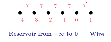
FIG. 1.: (Color online) Picture of a semi-infinite reservoir going from site number 0 to $-\infty$ and a wire beginning from site number 1.

The reservoir gives rise to a self-energy at the first site of the wire of the form [11, 23]

$$\Sigma(E)~{}=~{}\sigma(E)~{}\sum_{\sigma}~{}c_{1,\sigma}^{\dagger}c_{1,\sigma}~{},$$ (69)

where

$$\sigma(E)~{}=~{}-~{}\frac{\gamma^{\prime 2}}{\gamma}~{}e^{ik}$$ (70)

for $-2\gamma\leq E=-2\gamma\cos k\leq 2\gamma$ (with $0\leq k\leq\pi$),

$$\sigma(E)~{}=~{}-~{}\frac{\gamma^{\prime 2}}{\gamma}~{}e^{-k}~{}-~{}i\eta$$ (71)

for $E=-2\gamma\cosh k\leq-2\gamma$ (with $k\geq 0$), and

$$\sigma(E)~{}=~{}\frac{\gamma^{\prime 2}}{\gamma}~{}e^{-k}~{}-~{}i\eta$$ (72)

for $E=2\gamma\cosh k\geq 2\gamma$ (with $k\geq 0$). Here $\eta$ is an infinitesimal positive number which appears only if $E$ lies outside the range $[-2\gamma,2\gamma]$. For $-2\gamma<E<2\gamma$, the self-energy already has an imaginary piece, so it is not necessary to add an $i\eta$ term.

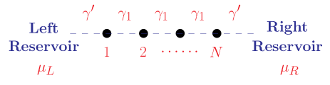
FIG. 2.: (Color online) A quantum wire system with a $N$-site wire in the middle and semi-infinite reservoirs on its left and right.

Now let us consider the complete system which consists of a wire with $N$ sites in the middle, and reservoirs on its left and right as shown in Fig. 2. If the wire is also modeled by a tight-binding Hamiltonian (with a hopping amplitude $\gamma_{1}$), the Green’s function of the wire at energy $E$ is given by a $N\times N$ matrix

$$G(E)~{}=~{}[~{}E~{}I~{}-~{}H~{}-~{}\Sigma_{L}(E)~{}-~{}\Sigma_{R}(E)~{}]^{-1}~{},$$ (73)

(74)

$$H~{}+~{}\Sigma_{L}(E)~{}+~{}\Sigma_{R}(E)~{}=$$ (75)

(76)

$$-~{}\left(\begin{array}[]{ccccc}{}\hfil\\ \sigma(E){}&~{}\gamma_{1}{}&~{}0{}&~{}\cdots{}&~{}\cdots{}\\ ~{}\gamma_{1}{}&~{}0{}&~{}\gamma_{1}{}&~{}0{}&~{}\cdots{}\\ ~{}0{}&~{}\gamma_{1}{}&~{}0{}&~{}\gamma_{1}{}&~{}0{}\\ ~{}\cdots{}&~{}\cdots{}&~{}\cdots{}&~{}\cdots{}&~{}\cdots{}\\ ~{}\cdots{}&~{}\cdots{}&~{}0{}&~{}\gamma_{1}{}&~{}\sigma(E){}\end{array}\right)~{}.$$ (83)

(The effects of the reservoirs on the wire is completely taken into account by the self-energy terms). We would like to emphasize that the relation between $E$ and $k$ is given entirely by the dispersion in the reservoirs (we assume that the dispersion is the same in both the reservoirs), and not on the form of the Hamiltonian $H$ inside the wire.

The density matrices due to electrons coming in from the left and right reservoirs are given by [11, 21, 22, 23]

$$\int~{}\frac{dE}{2\pi}~{}G\Gamma_{L}G^{\dagger}~{}f_{L}\quad{\rm and}\quad\int~{}\frac{dE}{2\pi}~{}G\Gamma_{R}G^{\dagger}~{}f_{R}$$ (84)

respectively, where $\Gamma_{a}(E)=i(\Sigma_{a}-\Sigma_{a}^{\dagger}),$

$$f_{a}(E)~{}=~{}[e^{\beta(E-\mu_{a})}+1]^{-1}$$ (85)

is the Fermi function, and $\mu_{a}~{}$ is the chemical potential in reservoir $a$. We note that if $E$ lies outside the range $[-2\gamma,2\gamma]$, the matrix $\Gamma_{a}(E)\sim 2\eta$ is infinitesimal. In that case, the density matrix can still receive a contribution from certain states; these are typically bound states which have a discrete set of energies $E_{b}$. The reason that such states can make a finite contribution in Eq. (84) even though $\Gamma_{a}$ is infinitesimal is that $G$ takes the form $1/(E-E_{b}+i\eta)$, and

$${\rm Lim}_{\eta\rightarrow 0^{+}}~{}\frac{2~{}\eta}{(E-E_{b})^{2}~{}+~{}\eta^{2}}~{}=~{}2~{}\pi~{}\delta(E-E_{b})~{}.$$ (86)

Finally, the current is given by the expression

$$I~{}=~{}-~{}\frac{e}{h}~{}\int~{}dE~{}{\rm trace}(G\Gamma_{L}G^{\dagger}\Gamma_{R})~{}[f_{L}(E)-f_{R}(E)]~{},$$ (87)

and the conductance is $G~{}=~{}e~{}I/(\mu_{L}~{}-~{}\mu_{R})~{}.$ If $E$ lies outside the range $[-2\gamma,2\gamma]$, $\Gamma_{L}(E)$ and $\Gamma_{R}(E)$ are both infinitesimal, and the current does not get any contribution from states lying in that energy range. (The difference between the density matrix and the current for such states is that the density matrix has only one factor of $\eta$ in the numerator while the current has two factors of $\eta$).

We will be interested below in the case of linear response, i.e, the limit $\mu_{L}\rightarrow\mu_{R}=\mu$. In that limit, the Fermi wavenumber $k_{F}$ is given by $\mu=-2\gamma\cos k_{F}$. Further, the conductance takes the form

$$G = \frac{e^{2}}{h}~{}\int_{-2\gamma}^{2\gamma}~{}dE~{}{\rm trace}(G\Gamma_{L}G^{\dagger}\Gamma_{R})~{}\frac{\beta}{[2~{}\cosh\frac{\beta}{2}(E-\mu)]^{2}}.$$ (88)

(We have to multiply the above expression by 2 for spin-half electrons).

B Interactions

Let us now consider how interactions can be studied within the NEGF formalism. Note that this formalism works with a one-particle Hamiltonian, e.g., the self-energy in Eq. (69) is given in terms of the energy of a single electron which is entering or leaving the wire. Hence, the only way to deal with interactions is to do a HF decomposition as shown in Eqs. (39) and (48); these take the form of corrections to the on-site chemical potential or the hopping amplitude.

However, there is a difficulty in using the expressions in (39) or (48). We want to have interactions between the electrons only in the wire, not in the reservoirs. The HF decompositions shown in (39) and (48) will then lead to one-body terms only in the wire; these terms will back-scatter electrons coming from the reservoirs, and hence reduce the conductance from its ideal value of $2e^{2}/h$ or $e^{2}/h$. We would like to ensure that there is no such scattering if there are no impurities inside the wire and if the leads connect adiabatically to the wires, i.e., if the entire system with wire and reservoirs is translation invariant. We know that two-body scatterings between electrons conserve momentum and therefore do not affect the conductance in the absence of impurities and scattering from the lead-wire junctions. We therefore modify the form of the HF decomposition from Eqs. (39) and (48) to Eqs. (LABEL:int4) and (LABEL:int6) respectively; the extra terms in those equations ensure that the HF terms vanish identically if there are no impurities. [An alternative way of ensuring adiabaticity between the leads and the wires is to turn on the interaction strength $U$ smoothly from zero in the leads to a finite value inside the wire. This, however, is harder to implement numerically. Subtracting the mean values as in (LABEL:int4) and (LABEL:int6) is easier to implement, and it serves the same purpose because the subtracted quantities approach zero near the ends of the wires (this will become clear from the numerical results presented below).]

In the presence of interactions, we will implement a self-consistent NEGF calculation as follows:

• Start with the Hamiltonian with no interactions, and calculate the density matrix. The diagonal elements of the density matrix give the densities at different sites.

• Use the HF approximation to compute the Hamiltonian with interactions, and use that to calculate the density matrix again.

• Repeat the previous step till the density changes no further, i.e., between two successive iterations, the maximum change in density on any lattice site is less than about $10^{-4}$.

• Use the converged density to compute the conductance.

V Numerical results

In this section, we will present the results obtained by the NEGF formalism, first for non-interacting electrons, and then for interacting spin-1/2 and spinless electrons, using the procedure described in Sec. IV B. We will study the dependence of the conductance $G$ on the wire length $L$, the inverse temperature $\beta$, the impurity strength $V$, and the interaction parameter $U$. Finally, we will make a quantitative comparison between our numerical results and the RG equations for the case of spinless electrons.

We present some details about our choice of parameters for the calculations. We always take the wire to have an odd number of sites, and the impurity to be on the middle site. The hopping amplitudes in the reservoirs and in the wire is chosen to be the same ($\gamma=\gamma_{1}=\gamma^{\prime}=1$); the values of the inverse temperature $\beta=1/(k_{B}T)$ is quoted in units of $1/\gamma$. (We set both $\hbar$ and the lattice spacing equal to 1). We choose $k_{F}=\pi/10$; hence, $v_{F}=2\sin k_{F}=0.618$, $\mu=-2\cos k_{F}=-1.902$, and $E_{F}=2(1-\cos k_{F})=0.098$. The thermal coherence length is given by $L_{T}=0.618\beta$. In the energy integrations for the current and conductance, we take the energy step size to be $dE=2\times 10^{-4}$. In the integration outside the energy range $[-2\gamma,2\gamma]$, we take the quantity $\eta$ to be 5 times $dE$. Finally, in all the figures, the conductance $G$ is expressed in units of $2e^{2}/h$ and $e^{2}/h$ for the spin-1/2 and spinless cases respectively.

Our choice of parameters was dictated partly by experiments on quantum wires in semiconductor heterojunctions [2, 3, 4, 5, 6, 7], and partly by our numerical limitations (which prevent us from going to very large wire lengths). Experimentally, the ratio of the wire length to the de Broglie wavelength of the electrons ($Lk_{F}/\pi$) ranges from about 20 to 200, the ratio of the wire length to the inverse temperature $L/\beta$ ranges from about 1/2 to 10, and the parameter $U/(2\pi v_{F})$ appearing in the Eq. (45) is about $0.2$ - $0.3$ [10]. In our calculations, $Lk_{F}/\pi$ goes from about 1 to 30, $L/\beta$ goes from about 1/40 to 6, and the interaction parameters take the values $U/(2\pi v_{F})=0.0773$ in the spin-1/2 case (Eq. (45)) and $(U/2\pi v_{F})[1-\cos(2k_{F})]=0.0148$ in the spinless case (Eq. (67)) for $U=0.3$. The much smaller value of the interaction parameter in the spinless case leads to smaller changes in the conductance in that case as we will see.

A Non-interacting electrons

Let us first discuss some properties of a system in which there is a $\delta$-function impurity of strength $V$ in the middle of the wire, and there are no interactions between the electrons. Fig. 3 shows the Friedel oscillations in the density $<c_{n}^{\dagger}c_{n}>$ for $V=0.3$ for two different temperatures. Note that the density at the middle site is much lower than the mean value of ${\bar{\rho}}=k_{F}/\pi=1/10$ due to the repulsive nature of the impurity. We also observe that the oscillations die out beyond a length scale of order $L_{T}=0.618\beta$ in the lower figure. This is a simple illustration of the idea of a thermal coherence length.

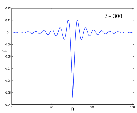
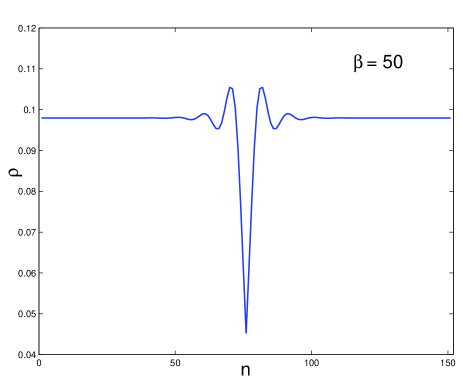
FIG. 3.: (Color online) Friedel oscillations in the density of non-interacting electrons caused by an impurity with $V=0.3$ placed in the middle of a wire with 151 sites. The upper and lower figures have $\beta=$ 300 and 50 respectively.

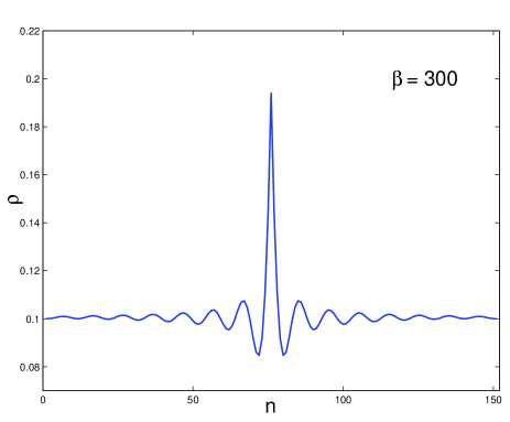
FIG. 4.: (Color online) Friedel oscillations in the density of non-interacting electrons caused by an impurity with $V=-0.3$ placed in the middle of a wire with 151 sites and $\beta=300$.

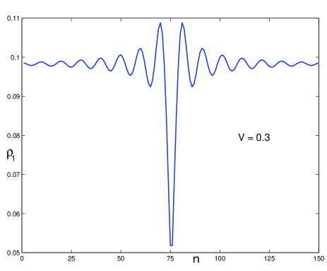
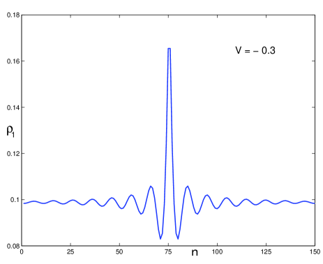
FIG. 5.: (Color online) Plots of $\rho_{1}\equiv<c_{n}^{\dagger}c_{n+1}>$ for non-interacting electrons in the presence of an impurity with $V=0.3$ (upper figure) and $-0.3$ (lower figure) placed in the middle of a wire with 151 sites, with $\beta=300$.

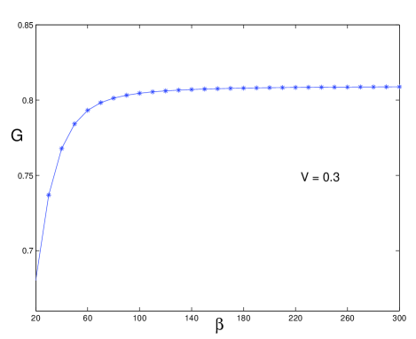
FIG. 6.: (Color online) Conductance versus $\beta$ for non-interacting electrons in the presence of an impurity with $V=0.3$ placed in the middle of a wire with 201 sites.

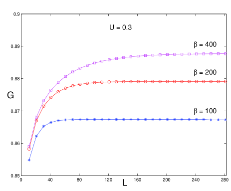
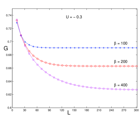
FIG. 7.: (Color online) Conductance versus wire length for interacting spin-1/2 electrons for three different values of $\beta$, for $V=0.3$. $U=$ 0.3 and -0.3 in the upper and lower figures respectively.

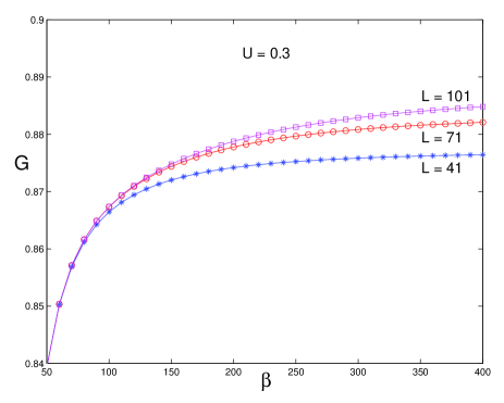
FIG. 8.: (Color online) Conductance versus $\beta$ for interacting spin-1/2 electrons for three different wire lengths, for $V=0.3$ and $U=0.3$.

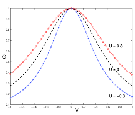
FIG. 9.: (Color online) Conductance $G$ versus $V$ for interacting spin-1/2 electrons for $U$ = 0.3, 0 and -0.3, with $L=101$ and $\beta=100$.

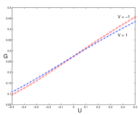
FIG. 10.: (Color online) Conductance $G$ versus $U$ for interacting spin-1/2 electrons for $V$ = 1 and -1, with $L=101$ and $\beta=100$.

Fig. 4 shows the Friedel oscillations in the density for $V=-0.3$ for $\beta=300$. The density in the middle site is now much higher than the mean value; this is because of the presence of a bound state whose wave function has a peak at that site. Indeed, in the absence of interactions, the difference in the site densities for $V=0.3$ and $-0.3$ is given entirely by the bound state. We see from Figs. 3 and 4 that the density difference at the site of the impurity is about 0.15; this agrees well with the value of $\tanh k_{b}=0.148$ given by Eq. (33). (For $V=-0.3$, we have $k_{b}=0.149$).

Finally, Fig. 5 shows the quantity $\rho_{1}\equiv<c_{n}^{\dagger}c_{n+1}>$ for $V=0.3$ and $-0.3$ for $\beta=300$. There is a strong similarity between these and the density plots shown in Figs. 3 (upper figure) and 4. This is because the electrons at the Fermi energy (which dominate the long distance properties of the system) have a wavelength which is $\pi/k_{F}=10$ times longer than the lattice spacing; hence there is very little difference between $<c_{n}^{\dagger}c_{n}>$ and $<c_{n}^{\dagger}c_{n+1}>$.

For non-interacting electrons, the conductance depends on the temperature, but not on the length of the wire. For a $\delta$-function impurity of strength $V$, the conductance for spinless electrons is given by

$$G = \frac{e^{2}}{h}~{}\int_{-2}^{2}~{}dE~{}{\cal T}(E)~{}\frac{\beta}{[2~{}\cosh\frac{\beta}{2}(E-\mu)]^{2}}~{},$$ (90)

$${\cal T}(E) = \frac{4\sin^{2}k}{4\sin^{2}k+V^{2}}~{}.$$ (91)

where $E=-2\cos k$. For $k_{B}T<<E_{F}=\mu+2$, Eq. (91) has a Sommerfeld expansion of the form [28]

$$G~{}=~{}\frac{e^{2}}{h}~{}[~{}T(\mu)~{}+~{}\frac{\pi^{2}}{6}~{}(k_{B}T)^{2}~{}T^{\prime\prime}(\mu)~{}+~{}\cdots~{}]~{}.$$ (92)

For $k_{F}=\pi/10$ and $V=0.3$, $T(\mu)=0.809$ and $(\pi^{2}/6)T^{\prime\prime}(\mu)=42.1$; this implies a significant temperature dependence of the conductance. Fig. 6 shows that the conductance changes appreciably with $\beta$ till $\beta$ reaches about 100. We have to keep this in mind when studying the temperature dependence of the conductance of a system of interacting electrons.

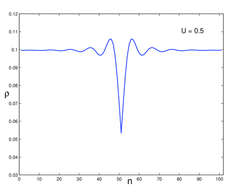
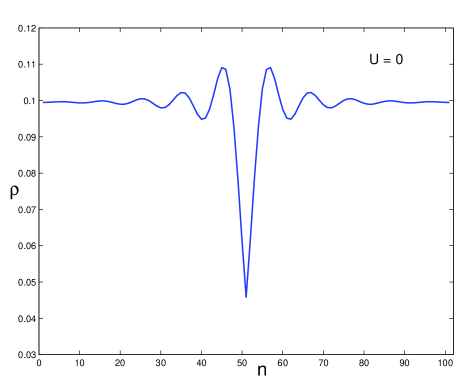
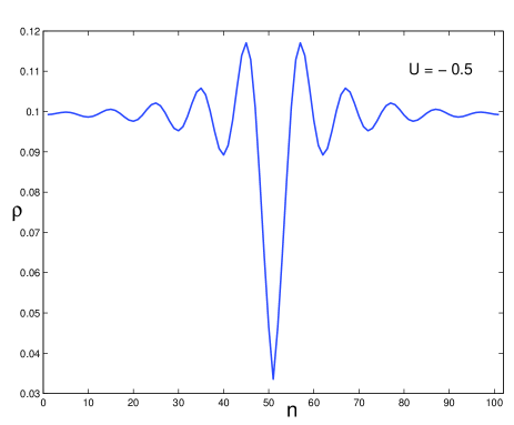
FIG. 11.: (Color online) Friedel oscillations for spin-1/2 electrons for $U=$ 0.5, 0 and -0.5 (upper, middle and lower figures respectively) for $V=0.3$, $L=101$ and $\beta=100$.

B Spin-1/2 electrons

We now consider the spin-1/2 model with an on-site interaction between the electrons. In the absence of interactions, the conductance at zero temperature is independent of the wire length and is given by Eq. (92), with a factor of 2 for spin; namely,

$$G_{0}~{}=~{}\frac{2e^{2}}{h}~{}\frac{4\sin^{2}k_{F}}{4\sin^{2}k_{F}~{}+~{}V^{2}}~{}.$$ (93)

For $k_{F}=\pi/10$ and $|V|=0.03$, $G_{0}=(2e^{2}/h)~{}0.809$.

In Fig. 7, we show the conductance as a function of the wire length $L$ for three different value of $\beta$, with $U=0.3$ in the upper figure and $U=-0.3$ in the lower figure. The trends in Fig. 7 are in accordance with Eq. (45). Firstly, the conductance increases with the length scale if $U>0$ and decreases if $U<0$. For $U=0.3$, we have $U/(2\pi v_{F})=0.0773$; we expect the HF approximation to be reasonable for such a small value. [Due to the RG flows of $g_{1}$ and $g_{2}$ in Eq. (25), the conductance should start decreasing for positive $U$ and increasing for negative $U$ at a very large length scale of the order of $L\sim\exp(1/0.0773)\sim 420000$, provided that $L_{T}$ is also larger than $420000$. Such a wire length is beyond our numerical capability.]

Secondly, for fixed $\beta$, $G$ increases till $L$ reaches a value of the order of $L_{T}=0.618\beta$ beyond which $G$ stops changing. This happens because there is complete thermal decoherence once $L$ exceeds $L_{T}$; hence $G$ does not vary any more with $L$ in that regime. Thirdly, the conductance for two different values of $\beta$, say, $\beta_{1}$ and $\beta_{2}$ (where $\beta_{1}<\beta_{2}$), start separating from each other at a value of the wire length $L_{c}$ such that $L_{c}/\beta_{1}$ is much less than $0.618$. This happens because if the inverse temperature is $\beta_{1}$ or higher, there is complete thermal coherence, and $G$ does not depend on $\beta$ any more. Thus, for any temperature $\beta$, there is a range of wire lengths going from $L_{c}$ up to $L_{T}$ where there is partial thermal coherence, and the conductance evolves slowly in this range of lengths. We therefore conclude that the RG flow does not suddenly stop at a length scale which is the smaller of the wire length $L$ and the thermal coherence length $L_{T}$; rather, the flow continues to occur (but slows down) in an intermediate range of length scales.

Finally, Fig. 7 shows that even for the smallest values of $L$, the conductance differs from the non-interacting value of $0.809$ by an appreciable amount. This is due to the large deviations of the density from the mean value at the sites close to the impurity. In that region, the density does not satisfy the $1/|n|$ form given in Eq. (38). Since that form is intimately tied to the RG results (the sum over $1/|n|$ gives $\ln(L)$), we do not expect the numerically obtained value of the conductance to agree well with the RG analysis for short wire lengths.

In Fig. 8, we show the conductance as a function of $\beta$ for three different value of $L$, with $U=0.3$. Once again, we see the same trends as in Fig. 7. Namely, for any two values of $L$, there is a $\beta$ where the values of $G$ start separating from each other. Then there is a higher value of $\beta$ where $G$ stops changing. The region between the two is where there is only partial thermal coherence, and $G$ varies relatively slowly in that region.

In Fig. 9, we show the conductance as a function of $V$ for three different values of $U$, with $L=101$ and $\beta=100$. Note that for $U=0$, the conductance is an even function of $V$ given by Eq. (93). But in the presence of interactions, $G$ is no longer precisely an even function of $V$, particularly for large values of $V$. This is more clearly visible in Fig. 10 which shows the conductance as a function of $U$ for $V=$ 1 and -1, with $L=101$ and $\beta=100$. For any value of $U$, we find that the conductance deviates less from the non-interacting value for $V>0$ compared to $V<0$, for the same value of $|V|$. For small values of $U$, this can be explained as follows. We saw in Figs. 3 and 4 that the density at the site of the impurity deviates from the mean density of ${\bar{\rho}}=1/10$ by a smaller amount for $V>0$ compared to $V<0$; the numerical values for $\rho_{0}-1/10$ are given by -0.046 and 0.095 for $V=$ 0.3 and -0.3 respectively. The effective impurity strength is given by

$$V_{\rm eff}~{}=~{}V~{}+~{}U~{}(\rho_{0}~{}-~{}{\bar{\rho}})~{},$$ (94)

which equals $0.3-0.046U$ and $-0.3+0.095U$ for $V=0.3$ and $-0.3$ respectively. For $U$ small and positive, this means that the magnitude of the effective impurity strength and therefore the reflection probability is larger for $V=0.3$; hence the conductance is smaller for $V=0.3$. The opposite statement is true if $U$ is small and negative. To conclude, the different values of the density deviation at the impurity site for positive and negative values of $V$ are responsible for the asymmetry in $G$ as a function of $V$. (This asymmetry is more prominent for the case of spinless electrons as we will see below).

The fact that the deviation of the conductance from the non-interacting value is smaller for $V>0$ than for $V<0$ is clearly a result of the bound state which raises the density at the impurity site for $V<0$; hence this is a short distance effect. [The contribution of the scattering states to the reflection probability $|r|^{2}$ is an even function of $V$ as one can see from Eq. (45). The RG equations which are derived from continuum theories take into account only long distance effects; these come from the scattering states only.]

In Fig. 11, we show the Friedel oscillations for three different values of $U$ with $V=0.3$, $L=101$ and $\beta=100$. We see that a repulsive interaction ($U>0$) suppresses the Friedel oscillations, while an attractive interaction ($U<0$) with the same magnitude enhances the oscillations by a much larger amount. This is because attractive interactions tend to lead to the formation of a charge density wave; if a charge density wave is already present (due to the impurity), attractive interactions enhance it. Since the scattering from the Friedel oscillations renormalize the scattering from the impurity, this difference in the magnitude of the oscillations helps to explain why the deviation of the conductance $G$ from the non-interacting value is larger for $U<0$ compared to $U>0$, as can be seen in Fig. 7.

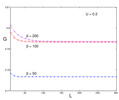
FIG. 12.: (Color online) Conductance versus wire length for interacting spinless electrons for three different values of $\beta$, for $V=0.3$ and $U=0.3$.

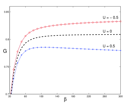
FIG. 13.: (Color online) Conductance versus $\beta$ for interacting spinless electrons for three different values of $U$, for a wire with 201 sites and $V=0.3$.

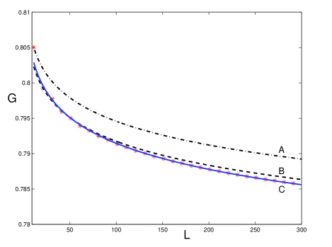
FIG. 14.: (Color online) Conductance $G$ versus $L$ for interacting spinless electrons compared with the RG expression in Eq. (16), for $V=0.3$, $U=0.3$, and $\beta=\infty$. Line A (dash dot line) corresponds to $d=11,~{}|t(d)|^{2}=0.805$ and $\alpha=0.0148$. Line B (dashed line) corresponds to $d=51,~{}|t(d)|^{2}=0.795$ and $\alpha=0.0148$. Line C (solid line) corresponds to $d=51,~{}|t(d)|^{2}=0.795$ and $\alpha=0.016$. The asterisks show the numerical results.

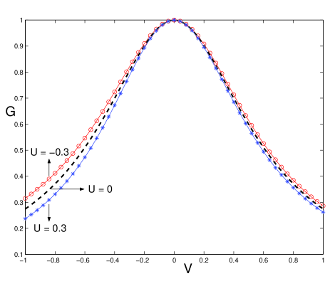
FIG. 15.: (Color online) Conductance $G$ versus $V$ for interacting spinless electrons for $U$ = 0.3, 0 and -0.3, with $L=101$ and $\beta=100$.

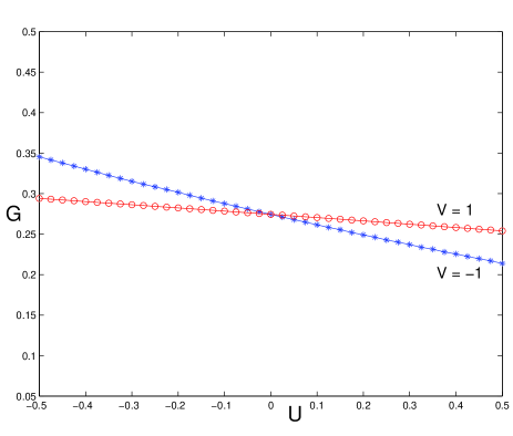
FIG. 16.: (Color online) Conductance $G$ versus $U$ for interacting spinless electrons for $V$ = 1 and -1, with $L=101$ and $\beta=100$.

For spin-1/2 electrons, we can do a self-consistent HF calculation in two ways, restricted and unrestricted. In a restricted HF calculation, the site densities of spin-up and spin-down electrons are taken to be equal at all stages. In a unrestricted HF calculation, spin-up and spin-down electrons are allowed to have different densities. We have done both kinds of calculations. For the range of the interaction $-0.5\leq U\leq 0.5$, we find that they give the same results; the spin-up and spin-down densities converge to the same values even if one begins with different initial values for them. Thus we do not find any spin density wave within our range of parameters.

C Spinless electrons

We now consider a model of spinless electrons with nearest neighbor interactions between the electrons. Comparing the forms of Eqs. (45) and (67), we see that the behaviors of the spin-1/2 model for $U>0$ and $U<0$ should be similar to that of the spinless model for $U<0$ and $U>0$ respectively. In Fig. 12, we show the conductance as a function of the wire length $L$ for three different value of $\beta$, with $V=0.3$ and $U=0.3$. The trends are in agreement with Eq. (45), with $\alpha=U(1-\cos(2k_{F}))/(2\pi v_{F})=0.0148$. For fixed $\beta$, $G$ decreases till $L$ reaches a value of the order of $L_{T}=0.618\beta$.

In Fig. 13, we show the conductance as a function of $\beta$ for three different value of $U$, with $V=0.3$ and $L=201$. As we saw earlier in Fig. 6, $G$ has a significant dependence on $\beta$ for small values of $\beta$ even for non-interacting electrons. It is only when we go to large values of $\beta$ that we see the trend expected from the RG equations for interacting electrons; namely, as $\beta$ increases, the conductance decreases if $U>0$ and increases if $U<0$.

Since $G$ has an appreciable dependence on $\beta$ even for non-interacting electrons, it is easier to consider the dependence of $G$ on the wire length $L$ at zero temperature in order to see how well the numerical results compare with the RG expression given in Eq. (16). That equation has two parameters, namely, the interaction parameter $\alpha$ and the short distance scale $d$ (with its corresponding transmission probability $|t(d)|^{2}$). To begin, let us choose $\alpha=0.0148$ as given by the analytical expression in Eq. (67) in terms of $U$ and $v_{F}$. In Fig. 14, we show a comparison between the expression in (16) for two values of $d$, namely, $d=11$ with $|t(d)|^{2}=0.805$ (the dash dot line A), and $d=51$ with $|t(d)|^{2}=0.795$ (the dashed line B), with our numerical results shown by astersisks. (The values of $|t(d)|^{2}$ for $d=$ 11 and 51 have themselves been obtained by our numerical calculations). We see that the RG expression with $d=51$ fits the numerical results better than the expression with $d=11$. This difference between the lines A and B shows that the interactions change the conductance by an appreciable amount between $d=11$ and $d=51$, and this change is not captured accurately by the expression in Eq. (16). [The conductance at short distances is affected substantially by quantities such as the large value of $\rho-{\bar{\rho}}$ at the site of the impurity. The RG analysis, on which (16) is based, does not take such effects into account.] Since the wavelength of the Friedel oscillations is given by $\lambda=10$, we conclude that the RG results agree reasonably well with the numerical results only if we begin the integration of the RG flows from a distance which is significantly larger than $\lambda$. However, we observe that even line B corresponding to $d=51$ starts deviating from the numerical results at large length scales. We have therefore tried varying the parameter $\alpha$ also, keeping $d$ and $|t(d)|^{2}$ fixed at $51$ and $0.795$ respectively. We find that $\alpha=0.016$ (the solid line C in Fig. 14) gives an excellent fit to the numerical results.

In Fig. 15, we show the conductance as a function of $V$ for three different values of $U$, with $L=101$ and $\beta=100$. We see that $G$ is not an even function of $V$ in the presence of interactions. In Fig. 16, we show the conductance as a function of $U$ for $V=$ 1 and -1, with $L=101$ and $\beta=100$. For any value of $U$, we again find that the conductance deviates less from the non-interacting value for $V=1$ compared to $V=-1$. The explanation for this is similar to that for the similar phenomenon in the spin-1/2 model, except that the roles of $U$ and $-U$ are interchanged in the two models. The larger change in the conductance for $V=-1$ is again due to the presence of a bound state.

VI Discussion

We have used the NEGF formalism to study the dependence of the conductance of a quantum wire with both spin-1/2 and spinless electrons on various parameters such as the wire length, temperature, impurity potential, and the strength of the interactions between the electrons. The advantage of the NEGF formalism is that it can be used to compute the density and conductance at any length scale. At large length scales, our numerical results agree with those obtained by an RG analysis of continuum theories. We find that the trends of the RG results can be understood using the Born approximation for scattering from a weak impurity and from the density oscillations produced by the impurity.

Our numerical results differ in detail in two ways from those obtained analytically from the RG equations. Firstly, the dependence of $G$ on the wire length and temperature fits the expression in Eq. (16) only if we take the starting point of the RG equation to be significantly larger than the short distance scale $\lambda$, and we allow $\alpha$ to be a little different from its analytically obtained value. Secondly, the conductance is not an even function of the impurity potential $V$ (as one expects from the RG analysis); this is due to the existence of a bound state for an attractive impurity. These differences between the numerical results and the results based on the RG analysis seem to be due to effects at short distances, where the density deviates significantly from the mean density.

Before ending, we would like to briefly compare our work with that of Refs. [17, 18, 19]. Using the functional RG technique, the authors of those papers have shown that there is excellent agreement at very large length scales between the numerical results and the asymptotic scaling forms given by the RG equations derived from continuum theories. We have not been able to go up to such large length scales using the NEGF formalism. However, even at the length scales studied by us, our numerical results agree quite well with the RG equations if we start at a short distance scale which is about 5 times larger than $\lambda$.

As mentioned towards the beginning of Sec. V, the length scales $L$ and $L_{T}$ that we have considered are comparable to those studied experimentally. Our observations about the short distance effects may therefore have implications for fitting experimental data to expressions obtained by an RG analysis.

Acknowledgments

We thank Supriyo Datta, Avik Ghosh and V. Ravi Chandra for many stimulating discussions. We thank the Department of Science and Technology, India for financial support under projects SR/FST/PSI-022/2000 and SP/S2/M-11/2000.

REFERENCES

- [1]
- [2] S. Tarucha, T. Honda, and T. Saku, Sol. St. Comm. 94, 413 (1995).
- [3] C. -T. Liang, M. Pepper, M. Y. Simmons, C. G. Smith, and D. A. Ritchie, Phys. Rev. B 61, 9952 (2000).
- [4] B. E. Kane, G. R. Facer, A. S. Dzurak, N. E. Lumpkin, R. G. Clark, L. N. Pfeiffer, and K. W. West, App. Phys. Lett. 72, 3506 (1998).
- [5] A. Yacoby, H. L. Stormer, N. S. Wingreen, L. N. Pfeiffer, K. W. Baldwin, and K. W. West, Phys. Rev. Lett. 77, 4612 (1996).
- [6] O. M. Auslaender, A. Yacoby, R. de Picciotto, K. W. Baldwin, L. N. Pfeiffer, and K. W. West, Phys. Rev. Lett. 84, 1764 (2000).
- [7] D. J. Reilly, G. R. Facer, A. S. Dzurak, B. E. Kane, R. G. Clark, P. J. Stiles, J. L. O’Brien, N. E. Lumpkin, L. N. Pfeiffer, and K. W. West, Phys. Rev. B 63, 121311(R) (2001).
- [8] C. L. Kane and M. P. A. Fisher, Phys. Rev. B 46, 15233 (1992).
- [9] A. Furusaki and N. Nagaosa, Phys. Rev. B 47, 4631 (1993).
- [10] S. Lal, S. Rao and D. Sen, Phys. Rev. Lett. 87, 026801 (2001); Phys. Rev. B 65, 195304 (2002).
- [11] S. Datta, Electronic transport in mesoscopic systems (Cambridge University Press, 1995).
- [12] Y. Imry, Introduction to Mesoscopic Physics (Oxford University Press, 1997).
- [13] C. S. Chu and R. S. Sorbello, Phys. Rev. B 40, 5941 (1989); Y. B. Levinson, M. I. Lubin, and E. V. Sukhorukov, Phys. Rev. B 45, 11936 (1992); E. Granot, Europhys. Lett. 68, 860 (2004).
- [14] D. Yue, L. I. Glazman, and K. A. Matveev, Phys. Rev. B 49, 1966 (1994); K. A. Matveev, D. Yue, and L. I. Glazman, Phys. Rev. Lett. 71, 3351 (1993).
- [15] S. Lal, S. Rao and D. Sen, Phys. Rev. B 66, 165327 (2002); S. Das, S. Rao and D. Sen, Phys. Rev. B 70, 085318 (2004).
- [16] D. G. Polyakov and I. V. Gornyi, Phys. Rev. B 68, 035421 (2003).
- [17] T. Enss, V. Meden, S. Andergassen, X. Barnabe-Theriault, W. Metzner, and K. Schönhammer, Phys. Rev. B 71, 155401 (2005).
- [18] S. Andergassen, T. Enss, V. Meden, W. Metzner, U. Schollwöck, and K. Schönhammer, Phys. Rev. B 70, 075102 (2004).
- [19] X. Barnabe-Theriault, A. Sedeki, V. Meden, and K. Schönhammer, Phys. Rev. B 71, 205327 (2005), and Phys. Rev. Lett. 94, 136405 (2005).
- [20] V. Meden and U. Schollwöck, Phys. Rev. B 67, 035106 (2003); V. Meden, W. Metzner, U. Schollwöck, O. Schneider, T. Stauber, and K. Schönhammer, Eur. Phys. J. B 16, 631 (2000).
- [21] Y. Meir and N. S. Wingreen, Phys. Rev. Lett. 68, 2512 (1992).
- [22] S. Datta, Superlattices and Microstructures 28, 253 (2000).
- [23] A. Dhar and B. S. Shastry, Phys. Rev. B 67, 195405 (2003).
- [24] M. Tsukada, K. Tagami, K. Hirose, and N. Kobayashi, J. Phys. Soc. Jpn. 74, 1079 (2005).
- [25] A. O. Gogolin, A. A. Nersesyan, and A. M. Tsvelik, Bosonization and Strongly Correlated Systems (Cambridge University Press, Cambridge, 1998); S. Rao and D. Sen, in Field Theories in Condensed Matter Physics, edited by S. Rao (Hindustan Book Agency, New Delhi, 2001); T. Giamarchi, Quantum Physics in One Dimension (Oxford University Press, Oxford, 2004).
- [26] E. Merzbacher, Quantum Mechanics (John Wiley & Sons, Singapore, 1999).
- [27] J. Solyom, Adv. Phys. 28, 201 (1979).
- [28] N. W. Ashcroft and N. D. Mermin, Solid State Physics (Holt, Rinehart and Winston, New York, 1976).