Effect of second-rank random anisotropy on critical phenomena of a random field O($N$) spin model in the large $N$ limit

Abstract

We study the critical behavior of a random field O($N$) spin model with a second-rank random anisotropy term in spatial dimensions $4<d<6$, by means of the replica method and the $1/N$ expansion. We obtain a replica-symmetric solution of the saddle-point equation, and we find the phase transition obeying dimensional reduction. We study the stability of the replica-symmetric saddle point against the fluctuation induced by the second-rank random anisotropy. We show that the eigenvalue of the Hessian at the replica-symmetric saddle point is strictly positive. Therefore, this saddle point is stable and the dimensional reduction holds in the $1/N$ expansion. To check the consistency with the functional renormalization group method, we obtain all fixed points of the renormalization group in the large $N$ limit and discuss their stability. We find that the analytic fixed point yielding the dimensional reduction is practically singly unstable in a coupling constant space of the given model with large $N$. Thus, we conclude that the dimensional reduction holds for sufficiently large $N$.

I Introduction

The random field O($N$) spin model is one of the simplest models with both a site randomness and a short range spin correlation. IM Despite intensive research for about three decades, our understanding of this model is not yet satisfactory (for recent review, see Ref. Na, ).

Dimensional reduction PS is one key to clarify the nature of this model. Dimensional reduction claims that the critical behavior of the $d$-dimensional random field O($N$) spin model is the same as of the $(d-2)$-dimensional pure O($N$) spin model, where $d$ is the spatial dimension. It has been shown by rigorous proofs I ; BK and numerical calculations of critical exponents Ri ; NB ; HY ; MF that the prediction of dimensional reduction is incorrect in the random field Ising model below four dimensions. In dimensions more than $4$, however, the critical phenomena of the random field O($N$) spin model should be further studied. In particular, the breakdown of the dimensional reduction and the possibility of an intermediate phase between the paramagnet and ferromagnet phasess are still under controversy.

Mézard and Young considered the possibility of the glassy phase by replica symmetry breaking. MY They dealt with the random field O($N$) $\phi^{4}$ model, and studied the critical behavior by using the replica method and the self-consistent screening approximation (SCSA), which is a truncated Schwinger-Dyson equation for a two-point correlation function. Under the assumption of replica symmetry, the dimensional reduction appears and the critical exponents of the connected and disconnected correlation functions $\eta$ and $\bar{\eta}$ satisfy $\bar{\eta}=\eta$. They showed that the replica-symmetric correlation function was, however, unstable as a solution of the SCSA equation at O($1/N$). They proposed a replica-symmetry-breaking correlation function, where they found $2\eta\sim\bar{\eta}$. Following Mézard and Young, the instability of the replica-symmetric solution against replica symmetry breaking has been reported in several papers. DOT ; AB However, the physical meaning of the instability in the SCSA equation is still unclear.

Fisher and Feldman pointed out the breakdown of the dimensional reduction due to the appearance of the infinite number of relevant operators near four dimensions. Fi ; Fe Fisher showed that all possible higher-rank random anisotropies are generated by the functional renormalization group recursion relations for the O($N$) nonlinear $\sigma$ model including only the random field term. The random field and the random anisotropies are marginal operators in $d=4$. Then he treated the nonlinear $\sigma$ model with a random field and all the random anisotropy terms, and calculated the one-loop beta function for a linear combination of them in $d=4+\epsilon$ under the assumption of replica symmetry. He showed that there is no singly unstable fixed point of O($\epsilon$) which gives the results of dimensional reduction, and that the flow goes into the regime where nonperturbative effects are important. Therefore, he concluded that the dimensional reduction breaks down at least near four dimensions. Feldman carefully reexamined the one-loop beta function obtained by Fisher. He treated a differential equation as the fixed point condition and found nonanalytic fixed points which control the critical phenomena instead of the analytic fixed ones. He calculated the exponents $\eta$ and $\bar{\eta}$ for $N=3,4,5$ in $4+\epsilon$ dimensions numerically; then he concluded that dimensional reduction breaks down near four dimensions for several finite $N$.

These studies indicate the breakdown of dimensional reduction in the random field O($N$) spin system. However, the relation between the renormalization group and simple $1/N$-expansion methods has never been discussed. Thus, it is important to study the relation between the stability of the replica-symmetric saddle point and the analytic fixed point in the functional renormalization group for large $N$.

In this paper, we study the random field O($N$) spin model including random anisotropy by a simple $1/N$ expansion and the functional renormalization group method. We study the robustness or fragility of the system against the random anisotropy perturbation. First, we study the stability of the replica-symmetric saddle point in spatial dimensions $4<d<6$ by the simple $1/N$ expansion. To investigate the stability of the replica-symmetric saddle point against a small perturbation of the second-rank random anisotropy, we employ the criterion for stability used by de Almeida and Thouless. AT We find that the eigenvalues of the Hessian are strictly positive, and the replica-symmetric saddle point remains stable against the second-rank random anisotropy. Therefore, the dimensional reduction works well for large $N$. Next, we check the consistency of this result with the functional renormalization group analysis in $4+\epsilon$ dimensions. We solve the fixed point condition of the renormalization group in the large $N$ limit, and study the stability of all fixed points. We solve the eigenvalue equation for the infinitesimal deviation from the fixed points. We find that the analytic fixed point yielding dimensional reduction is singly unstable. Careful analysis of the eigenvalue equation for the infinitesimal deviation from this fixed point is done in terms of $1/N$ expansion. We find infinitely many unphysical modes which should be eliminated. In practice, the analytic fixed point yielding the dimensional reduction is singly unstable for sufficiently large $N$. Therefore, our simple $1/N$ expansion is consistent with the functional renormalization group method and we conclude the dimensional reduction

$$\eta=\bar{\eta}=\frac{d-4}{N-2}$$

for sufficiently large $N$.

This paper is organized as follows. In Sec. II, we briefly review the large $N$ behavior of the random field O($N$) spin model in the absence of random anisotropy. In Sec. III, we introduce the second-rank random anisotropy term, and perform the $1/N$ expansion for the random field O($N$) spin model with the second-rank random anisotropy term. We should integrate over the “off-diagonal” fluctuation introduced through the Hubbard-Stratonovich transformation for the second-rank random anisotropy. Solving the saddle-point equations under the assumption of replica symmetry, we have two solutions. Then we calculate the free energy densities at high temperatures in both solutions, and compare with the result of the high temperature expansion without the replica method. As a result, the solution is uniquely determined. Details of the calculations of the free energy at high temperatures without the replica method are relegated to Appendix A. We also calculate the critical line, and the eigenvalue of the Hessian at high temperature and near the critical point. The stability of the replica-symmetric saddle point is investigated. Details of the calculations of the eigenvalue of the Hessian are relegated to Appendix B. In Sec. IV, we compare our results with those of a renormalization group study. Technical details of the renormalization group for large $N$ are presented in Appendix C. Finally in Sec. V we summarize the results obtained in this paper, give some comments on the critical phenomena of both the lower and the upper critical dimensions on the basis of the results, and mention future problems. Calculation of loop integrals is exhibited in Appendix D.

II Critical behavior of random field O($N$) spin model in the large $N$ limit

In this section, we briefly review the $1/N$ expansion for the O($N$) spin model with only a random magnetic field under the assumption of replica symmetry. The stability of the replica symmetric saddle point is studied.

We consider the random field O($N$) spin model on a $d$-dimensional hypercubic lattice with the lattice spacing unity. Let $L$ be the linear length of the $d$-dimensional hypercubic lattice, and $V$ the number of lattice sites ($V=L^{d}$). The Hamiltonian is given by

$$H=-J\sum_{\langle x,y\rangle}{\mbox{\boldmath$S$}}_{x}\cdot{\mbox{\boldmath$S$}}_{y}-\sum_{x}{\mbox{\boldmath$h$}}_{x}\cdot{\mbox{\boldmath$S$}}_{x}.$$ (1)

Here $\langle x,y\rangle$ denotes the summation over the nearest neighbor pairs of the lattice sites $x$ and $y$. $J$ is the exchange interaction, and we take $J>0$. ${\mbox{\boldmath$S$}}_{x}$ denotes an $N$-component spin variable on the site $x$ with a fixed-length constraint ${\mbox{\boldmath$S$}}_{x}^{2}=1$, and ${\mbox{\boldmath$h$}}_{x}$ denotes a Gaussian random field with zero average. Taking the average over the random fields $\{{\mbox{\boldmath$h$}}_{x}\}$ by using the replica method, we have the following replica partition function:

$${\cal{Z}}\!\!\! = \!\!\!e^{nV\beta Jd}$$ (2)

$$\!\!\!\times\int\biggl{(}\prod_{x}\prod_{\alpha=1}^{n}\sqrt{N}d{\mbox{\boldmath$S$}}_{x,\alpha}\delta({{\mbox{\boldmath$S$}}_{x,\alpha}}^{2}-1)\biggr{)}e^{-\beta H_{\rm rep}},$$

$$\beta H_{\rm rep}=\frac{\beta}{2}\sum_{x}\sum_{\alpha,\beta}^{n}{\mbox{\boldmath$S$}}_{x,\alpha}(-J\widehat{\Delta}_{x}\delta_{\alpha\beta}-\beta\Delta){\mbox{\boldmath$S$}}_{x,\beta}.$$ (3)

Here $\widehat{\Delta}_{x}$ stands for the lattice Laplacian. In the momentum representation, the lattice Laplacian is represented by $\widehat{\Delta}_{k}=2\sum_{\mu=1}^{d}(\cos k_{\mu}-1)$. $\beta$ is the inverse temperature, and $T$ is the temperature; $\beta=1/kT$. $\Delta$ denotes the strength of the Gaussian random field. The replica index is denoted by $\alpha=1,...,n$. We rewrite $\delta({{\mbox{\boldmath$S$}}_{x,\alpha}}^{2}-1)$ in terms of the auxiliary variable $\lambda_{\alpha x}$:

$$\delta({{\mbox{\boldmath$S$}}_{x,\alpha}}^{2}-1)=\int_{-\infty}^{\infty}\frac{\beta d\lambda_{\alpha x}}{4\pi}e^{-\beta i\lambda_{\alpha x}({{\mbox{\boldmath$S$}}_{x,\alpha}}^{2}-1)/2}.$$ (4)

After integrating over the spin variables $\{{{\mbox{\boldmath$S$}}_{x,\alpha}}\}$, the replica partition function becomes

$${\cal{Z}} = e^{nV\beta Jd}\biggl{(}\frac{\beta}{4\pi}\biggr{)}^{nV}\biggl{(}\frac{2\pi N}{\beta}\biggr{)}^{NnV/2}$$ (5)

$$\times\int\biggl{(}\prod_{x}\prod_{\alpha=1}^{n}d\lambda_{\alpha x}\biggr{)}e^{-S_{\rm eff}},$$

$$S_{\rm eff} = \frac{N}{2}\sum_{x}\langle x|{\rm Tr}\ln(-J\widehat{\Delta}_{x}{\mbox{\boldmath$1$}}_{n}+{\mbox{\boldmath$\chi$}})|x\rangle$$ (6)

$$-\frac{\beta}{2}\sum_{x}\sum_{\alpha=1}^{n}i\lambda_{\alpha x},$$

where ${\mbox{\boldmath$1$}}_{n}$ is an $n\times n$ unit matrix, and $\chi$ is an $n\times n$ symmetric matrix with

$$\chi_{\alpha\beta x}=i\lambda_{\alpha x}\delta_{\alpha\beta}-\beta\Delta.$$ (7)

We study the large $N$ limit below. The large $N$ limit is taken with $NT$ (or $\beta/N$) and $N\Delta$ finite. Then, we redefine the parameters as follows:

$$NT\rightarrow T\,\,\,\,\biggl{(}\frac{\beta}{N}\rightarrow\beta\biggr{)},$$ (8)

$$N\Delta\rightarrow\Delta.$$

Thus, the replica partition function is rewritten as follows:

$${\cal{Z}} = e^{NnV\beta Jd}\biggl{(}\frac{N\beta}{4\pi}\biggr{)}^{nV}\biggl{(}\frac{2\pi}{\beta}\biggr{)}^{NnV/2}$$ (9)

$$\times\int\biggl{(}\prod_{x}\prod_{\alpha=1}^{n}d\lambda_{\alpha x}\biggr{)}e^{-S_{\rm eff}},$$

$$S_{\rm eff} = \frac{N}{2}\sum_{x}\langle x|{\rm Tr}\ln(-J\widehat{\Delta}_{x}{\mbox{\boldmath$1$}}_{n}+{\mbox{\boldmath$\chi$}})|x\rangle$$ (10)

$$-\frac{N\beta}{2}\sum_{x}\sum_{\alpha=1}^{n}i\lambda_{\alpha x}.$$

II.1 Saddle-point equation and replica-symmetric approximation

Differentiating $S_{\rm eff}$ by $i\lambda_{\alpha x}$, we get the saddle-point equation

$$\frac{\delta S_{\rm eff}}{\delta i\lambda_{\alpha x}}=\frac{N}{2}\biggl{\langle}x\biggr{|}\biggl{(}\frac{1}{-J\widehat{\Delta}_{x}{\mbox{\boldmath$1$}}_{n}+{\mbox{\boldmath$\chi$}}}\biggr{)}_{\alpha\alpha}\biggl{|}x\biggr{\rangle}-\frac{N\beta}{2}=0.$$ (11)

Here we assume the replica symmetry

$$i\lambda_{\alpha x}=m^{2}.$$ (12)

In this assumption,

$$\biggl{\langle}k\biggr{|}\biggl{(}\frac{1}{-J\widehat{\Delta}_{k}{\mbox{\boldmath$1$}}_{n}+{\mbox{\boldmath$\bar{\chi}$}}}\biggr{)}_{\alpha\beta}\biggl{|}k\biggr{\rangle}$$

$$=\frac{1}{-J\widehat{\Delta}_{k}+m^{2}}\delta_{\alpha\beta}+\frac{\beta\Delta}{(-J\widehat{\Delta}_{k}+m^{2})^{2}}$$

$$\equiv G_{0k}^{\rm c}\delta_{\alpha\beta}+\beta\Delta G_{0k}^{\rm d}\equiv G_{0k}^{\alpha\beta}.$$ (13)

The saddle-point equation becomes

$$1=\frac{1}{\beta}a(m^{2})+\Delta b(m^{2}),$$ (14)

where

$$a(m^{2}) = \frac{1}{V}\sum_{k}\frac{1}{-J\widehat{\Delta}_{k}+m^{2}},$$ (15)

$$b(m^{2}) = \frac{1}{V}\sum_{k}\frac{1}{(-J\widehat{\Delta}_{k}+m^{2})^{2}}.$$ (16)

In the thermodynamic limit $V\to\infty$, $a(m^{2})$ and $b(m^{2})$ change over the integrals:

$$a(m^{2}) \stackrel{{\scriptstyle V\rightarrow\infty}}{{=}} \int_{k\in[-\pi,\pi]^{d}}\frac{d^{d}k}{(2\pi)^{d}}\frac{1}{-J\widehat{\Delta}_{k}+m^{2}},$$ (17)

$$b(m^{2}) \stackrel{{\scriptstyle V\rightarrow\infty}}{{=}} \int_{k\in[-\pi,\pi]^{d}}\frac{d^{d}k}{(2\pi)^{d}}\frac{1}{(-J\widehat{\Delta}_{k}+m^{2})^{2}},$$ (18)

$$\int_{k\in[-\pi,\pi]^{d}}\frac{d^{d}k}{(2\pi)^{d}}\equiv\prod_{\mu=1}^{d}\biggl{(}\int_{-\pi}^{\pi}\frac{dk_{\mu}}{2\pi}\biggr{)}.$$ (19)

Near the critical point, $m$ becomes small, and then the integrals (17) and (18) can be expanded in terms of $m$ for $4<d<6$,

$$a(m^{2}) \simeq a_{0}-a_{1}m^{2},$$ (20)

$$b(m^{2}) \simeq b_{0}-b_{1}m^{d-4},$$ (21)

where $a_{0}$, $a_{1}$, $b_{0}$, and $b_{1}$ are positive constants. The derivation of these is shown in Appendix D. Inserting the above expansions into the right hand side of Eq. (14), we get

$$1=kT(a_{0}-a_{1}m^{2})+\Delta(b_{0}-b_{1}m^{d-4}).$$ (22)

At first, we study two special cases: one is the $\Delta=0$ case, and the other is the $T=0$ case. Putting $\Delta=0$, we have the following expression for the saddle point $m$:

$$m^{2}=\frac{a_{0}}{a_{1}}\frac{T-T_{c}^{\rm(pure)}}{T},$$ (23)

$$kT_{c}^{\rm(pure)}=\frac{1}{a_{0}}.$$ (24)

This indicates

$$\xi \sim m^{-1}\sim(T-T_{c}^{\rm(pure)})^{-\nu},$$ (25)

$$\nu = \frac{1}{2}.$$ (26)

This result is identical with that of the mean field theory of the pure system as expected. In the case of $T=0$, $m$ is expressed as follows:

$$m^{d-4}=\frac{b_{0}}{b_{1}}\frac{\Delta-\Delta_{c}^{(T=0)}}{\Delta},$$ (27)

$$\Delta_{c}^{(T=0)}=\frac{1}{b_{0}}.$$ (28)

This indicates

$$\xi \sim m^{-1}\sim(\Delta-\Delta_{c}^{(T=0)})^{-\nu},$$ (29)

$$\nu = \frac{1}{d-4}.$$ (30)

In $d=4+\epsilon$, the above result agrees with that of pure systems in $d=2+\epsilon$ in the leading order. Next, we study the case of $T\neq 0$ and $\Delta\neq 0$. The saddle point $m$ is expressed as follows:

$$m=\biggl{(}\frac{1}{\Delta b_{1}}(kTa_{0}+\Delta b_{0}-1)\biggr{)}^{1/(d-4)}.$$ (31)

Putting $m=0$, we can get the critical line between ferromagnetic and paramagnetic phases:

$$kT_{c}a_{0}+\Delta_{c}b_{0}=1,$$ (32)

$$\frac{\Delta_{c}}{\Delta_{c}^{(T=0)}}+\frac{T_{c}}{T_{c}^{\rm(pure)}}=1.$$ (33)

The phase diagram is depicted in Fig. 1.

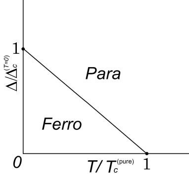
Figure 1: Phase diagram of the random field O($N$) model

$m$ is rewritten by using $T_{c}$ and $\Delta_{c}$ as follows:

$$m = \biggl{[}\frac{1}{\Delta b_{1}}\biggl{(}\frac{T-T_{c}}{T_{c}^{\rm(pure)}}+\frac{\Delta-\Delta_{c}}{\Delta_{c}^{(T=0)}}\biggr{)}\biggr{]}^{1/(d-4)}$$ (36)

$$\simeq \left\{\begin{array}[]{lc}(T-T_{c})^{1/(d-4)}&(\Delta=\Delta_{c}),\\ (\Delta-\Delta_{c})^{1/(d-4)}&(T=T_{c}).\end{array}\right.$$

This indicates

$$\xi \sim m^{-1}\sim(\Delta-\Delta_{c})^{-\nu}\sim(T-T_{c})^{-\nu},$$ (37)

$$\nu = \frac{1}{d-4}.$$ (38)

In $d=4+\epsilon$, this result is identical with that of pure systems in $d=2+\epsilon$ in the leading order.

II.2 Stability of replica-symmetric saddle point

We put

$$\chi_{\alpha\beta x} = (m^{2}\delta_{\alpha\beta}-\beta\Delta)+i\epsilon_{\alpha x}\delta_{\alpha\beta}$$ (39)

$$\equiv \bar{\chi}_{\alpha\beta}+\delta\chi_{\alpha\beta x},$$

and expand the effective action $S_{\rm eff}$ up to the second order of $\delta\chi_{\alpha\beta x}$. The second-order term of $\delta\chi_{\alpha\beta x}$ for the effective action $S_{\rm eff}$ becomes

$$\delta^{2}\!S_{\rm eff}\!\!\! = \!\!\!-\frac{N}{4}\!\!\int\!\!d^{d}\!x\biggl{\langle}\!x\biggr{|}{\rm Tr}\frac{1}{-J\widehat{\Delta}_{x}{\mbox{\boldmath$1$}}_{n}\!\!+\!{\mbox{\boldmath$\bar{\chi}$}}}\delta\chi\frac{1}{-J\widehat{\Delta}_{x}{\mbox{\boldmath$1$}}_{n}\!\!+\!{\mbox{\boldmath$\bar{\chi}$}}}\delta\chi\biggl{|}x\!\biggr{\rangle}$$ (40)

$$= \!\!\!\frac{N}{4}\int_{k\in[-\pi,\pi]^{d}}\frac{d^{d}k}{(2\pi)^{d}}\sum_{\alpha,\beta}^{n}\epsilon_{\alpha k}\epsilon_{\beta,-k}\Pi_{\alpha\beta k}$$

$$= \!\!\!\frac{N}{4}\int_{k\in[-\pi,\pi]^{d}}\frac{d^{d}k}{(2\pi)^{d}}{}^{t}{\mbox{\boldmath$\epsilon$}}_{k}\hat{\Pi}_{k}{\mbox{\boldmath$\epsilon$}}_{-k},$$

in the thermodynamic limit. $\Pi_{\alpha\beta k}$ is

$$\Pi_{\alpha\beta k}\!\!\! = \!\!\!\int_{q\in[-\pi,\pi]^{d}}\frac{d^{d}q}{(2\pi)^{d}}G_{0k-q}^{\alpha\beta}G_{0q}^{\beta\alpha}$$ (41)

$$= [(A*A)_{k}+(A*B)_{k}+(B*A)_{k}]\delta_{\alpha\beta}+(B*B)_{k}$$

$$\equiv \Pi_{ck}\delta_{\alpha\beta}+\Pi_{dk},$$

$$(A*A)_{k} = \int_{q\in[-\pi,\pi]^{d}}\frac{d^{d}q}{(2\pi)^{d}}G_{0k-q}^{\rm c}G_{0q}^{\rm c},$$ (42)

$$(A*B)_{k} = (B*A)_{k}$$ (43)

$$= \beta\Delta\int_{q\in[-\pi,\pi]^{d}}\frac{d^{d}q}{(2\pi)^{d}}G_{0k-q}^{\rm c}G_{0q}^{\rm d},$$

$$(B*B)_{k} = (\beta\Delta)^{2}\int_{q\in[-\pi,\pi]^{d}}\frac{d^{d}q}{(2\pi)^{d}}G_{0k-q}^{\rm d}G_{0q}^{\rm d}.$$ (44)

The expression ${\mbox{\boldmath$\epsilon$}}_{k}$ is an $n$-dimensional vector whose elements are $\epsilon_{\alpha k}$:

$${\mbox{\boldmath$\epsilon$}}_{k}=\left(\begin{array}[]{c}\epsilon_{1k}\\ \epsilon_{2k}\\ \vdots\\ \epsilon_{nk}\\ \end{array}\right),$$ (49)

and $\hat{\Pi}_{k}$ denotes an $n\times n$ matrix whose elements are $\Pi_{\alpha\beta k}$:

$$\hat{\Pi}_{k}=\left(\begin{array}[]{cccc}\Pi_{ck}+\Pi_{dk}&\Pi_{dk}&\cdots&\Pi_{dk}\\ \Pi_{dk}&\Pi_{ck}+\Pi_{dk}&\cdots&\Pi_{dk}\\ \vdots&\vdots&\ddots&\vdots\\ \Pi_{dk}&\Pi_{dk}&\cdots&\Pi_{ck}+\Pi_{dk}\\ \end{array}\right).$$ (54)

Calculating the eigenvalues of the matrix $\hat{\Pi}_{k}$, we have

$$\lambda_{k,n}=\left\{\begin{array}[]{lcc}\Pi_{ck}+n\Pi_{dk},&&\\ \Pi_{ck}.&&\end{array}\right.$$ (57)

Taking the $n\rightarrow 0$ limit, we can obtain the following expression for the eigenvalue:

$$\lambda_{k} \equiv \lim_{n\rightarrow 0}\lambda_{k,n}=\Pi_{ck}$$

$$= \int_{q\in[-\pi,\pi]^{d}}\frac{d^{d}q}{(2\pi)^{d}}(G_{0k-q}^{\rm c}G_{0q}^{\rm c}+2\beta\Delta G_{0k-q}^{\rm c}G_{0q}^{\rm d}).$$

Therefore the eigenvalue $\lambda_{k}$ is positive for $T\geq 0$ and all $k$. This result indicates that the replica-symmetric saddle point is stable against “diagonal”fluctuations $\epsilon_{\alpha k}$, and therefore it is possible to integrate out the fluctuations $\epsilon_{\alpha k}$.

As seen in Eq. (39), the field includes no “off-diagonal”terms. In the next section, we shall study the effects of a second-rank random anisotropy on the critical phenomena of the random field O($N$) spin model. We will find that the off-diagonal fluctuation is introduced through the Hubbard-Stratonovich transformation for the second-rank random anisotropy term.

II.3 Calculation of $\eta$ and $\bar{\eta}$ in $4+\epsilon$ dimensions

Here, we calculate the critical exponents $\eta$ and $\bar{\eta}$. For simplicity, we put $J=1$. At criticality, the lattice Laplacian becomes $\widehat{\Delta}_{k}=-k^{2}$. Eq. (41) is

$$\Pi_{\alpha\beta k}=(c_{0}+c_{1}k^{d-4}+c_{2}k^{d-6})\delta_{\alpha\beta}+c_{3}k^{d-8},$$ (59)

for $m^{2}=0$, where

$$c_{0}=\int\frac{d^{d}q}{(2\pi)^{d}}\frac{1}{q^{4}},$$

$$c_{1}=\frac{1}{(4\pi)^{d/2}}\frac{\Gamma(\frac{6-d}{2})[2\Gamma(\frac{d-2}{2})^{2}-\frac{1}{2}\Gamma(\frac{d-4}{2})^{2}]}{\Gamma(d-4)},$$

$$c_{2}=\frac{2\Delta}{(4\pi)^{d/2}}\frac{\Gamma(\frac{6-d}{2})}{\Gamma(d-3)}\Gamma\biggl{(}\frac{d-2}{2}\biggr{)}\Gamma\biggl{(}\frac{d-4}{2}\biggr{)},$$

$$c_{3}=\frac{\Delta^{2}}{(4\pi)^{d/2}}\frac{\Gamma(\frac{8-d}{2})}{\Gamma(d-4)}\Gamma\biggl{(}\frac{d-4}{2}\biggr{)}^{2}.$$ (60)

Let us compute the correlation function at the second order of the perturbation. Up to the second order of $\epsilon_{\alpha k}$, we get the following expression for the correlation function:

$$G_{p}^{\alpha\beta}\!\!\! = \!\!\!\frac{1}{{\cal{Z}}_{\epsilon}}\biggl{(}\int\prod_{\alpha=1}^{n}{\cal{D}}\epsilon_{\alpha}\biggr{)}\biggl{\langle}p\biggr{|}\biggl{(}\frac{1}{-\partial^{2}{\mbox{\boldmath$1$}}_{n}+{\mbox{\boldmath$\chi$}}}\biggr{)}_{\alpha\beta}\biggl{|}p\biggr{\rangle}$$ (61)

$$\!\!\!\times\exp(-\delta^{2}S_{\rm eff})$$

$$\simeq \!\!\!G_{0p}^{\alpha\beta}-\sum_{\gamma,\delta}^{n}G_{0p}^{\alpha\gamma}\int\frac{d^{d}q}{(2\pi)^{d}}G_{0p-q}^{\gamma\delta}\langle\epsilon_{\gamma q}\epsilon_{\delta,-q}\rangle_{\epsilon}G_{0p}^{\delta\beta}$$

$$= \!\!\!G_{0p}^{\alpha\beta}-\sum_{\gamma,\delta}^{n}G_{0p}^{\alpha\gamma}\Sigma_{p}^{\gamma\delta}G_{0p}^{\delta\beta}$$

$$\simeq \!\!\!G_{0p}^{\alpha\beta}-\sum_{\gamma,\delta}^{n}G_{0p}^{\alpha\gamma}\Sigma_{p}^{\gamma\delta}G_{p}^{\delta\beta},$$

where ${\cal{Z}}_{\epsilon}$, $\Sigma_{p}^{\gamma\delta}$, and $\langle\epsilon_{\gamma q}\epsilon_{\delta,-q}\rangle_{\epsilon}$ are defined by

$${\cal{Z}}_{\epsilon}=\biggl{(}\int\prod_{\alpha=1}^{n}{\cal{D}}\epsilon_{\alpha}\biggr{)}\exp(-\delta^{2}S_{\rm eff}),$$

$$\Sigma_{p}^{\gamma\delta}\equiv\int\frac{d^{d}q}{(2\pi)^{d}}G_{0p-q}^{\gamma\delta}\langle\epsilon_{\gamma q}\epsilon_{\delta,-q}\rangle_{\epsilon},$$ (62)

$$\langle\epsilon_{\gamma q}\epsilon_{\delta,-q}\rangle_{\epsilon}\!\!\! \equiv \!\!\!\frac{1}{{\cal{Z}}_{\epsilon}}\biggl{(}\int\prod_{\alpha=1}^{n}{\cal{D}}\epsilon_{\alpha}\biggr{)}\epsilon_{\gamma q}\epsilon_{\delta,-q}\exp(-\delta^{2}S_{\rm eff})$$ (63)

$$= \!\!\!\frac{2}{N}\biggl{(}\frac{\delta_{\gamma\delta}}{c_{0}+c_{1}q^{d-4}+c_{2}q^{d-6}}$$

$$\!\!\!-\frac{c_{3}q^{d-8}}{(c_{0}+c_{1}q^{d-4}+c_{2}q^{d-6})^{2}}\biggr{)}.$$

In $4<d<6$ and in low momentum, $\langle\epsilon_{\gamma q}\epsilon_{\delta,-q}\rangle_{\epsilon}$ becomes

$$\langle\epsilon_{\gamma q}\epsilon_{\delta,-q}\rangle_{\epsilon}\sim\frac{2}{Nc_{2}}\biggl{(}\frac{1}{q^{d-6}}\delta_{\gamma\delta}-\frac{6-d}{2}\frac{\Delta}{q^{d-4}}\biggr{)}.$$ (64)

Thus, we get the following vertex function:

$$(G_{p}^{-1})_{\alpha\beta} = (p^{2}+m^{2})\delta_{\alpha\beta}-\Delta+\Sigma_{p}^{\alpha\beta}$$ (65)

$$= (p^{2}+m_{\rm R}^{2})\delta_{\alpha\beta}-\Delta_{\rm R}+\Sigma_{p}^{\alpha\beta}-\Sigma_{0}^{{}^{\prime}\alpha\beta},$$

where $\Sigma_{0}^{{}^{\prime}\alpha\beta}$, $m_{\rm R}$, and $\Delta_{\rm R}$ are defined by

$$\Sigma_{0}^{{}^{\prime}\alpha\beta}=\Sigma_{0}^{\alpha\beta}-\int d^{d}q\frac{\Delta^{2}(6-d)}{2(q^{2}+m^{2})^{2}q^{d-4}},$$

$$m^{2}\delta_{\alpha\beta}-\Delta\equiv m_{\rm R}^{2}\delta_{\alpha\beta}-\Delta_{\rm R}-\Sigma_{0}^{{}^{\prime}\alpha\beta}.$$ (66)

$\Sigma_{0}^{{}^{\prime}\alpha\beta}$ does not include an infrared divergence. At the criticality $m_{\rm R}^{2}=0$, we have

$$(G_{p}^{-1})_{\alpha\beta}=p^{2}\delta_{\alpha\beta}-\Delta_{\rm R}+\Sigma_{p}^{\alpha\beta}-\Sigma_{0}^{{}^{\prime}\alpha\beta}.$$ (67)

$\Sigma_{p}^{\alpha\beta}-\Sigma_{0}^{{}^{\prime}\alpha\beta}$ is calculated as follows:

$$\Sigma_{p}^{\alpha\beta}-\Sigma_{0}^{{}^{\prime}\alpha\beta} = \int\frac{d^{d}q}{(2\pi)^{d}}(G_{0p-q}^{\alpha\beta}-G_{0q}^{\alpha\beta})\langle\epsilon_{\alpha q}\epsilon_{\beta,-q}\rangle_{\epsilon}$$ (68)

$$= \frac{2}{Nc_{2}}(D_{p}\delta_{\alpha\beta}-E_{p}),$$

where $D_{p}$ and $E_{p}$ are

$$D_{p} = \frac{\Delta}{2}\frac{1}{(4\pi)^{d/2}}\frac{d-6}{\Gamma(d/2)}p^{2}\ln p^{2},$$

$$E_{p} = \frac{\Delta^{2}}{2}\frac{1}{(4\pi)^{d/2}}\frac{d-6}{\Gamma(d/2)}\ln p^{2}.$$ (69)

Thus, we get the following expression for the vertex function:

$$(G_{p}^{-1})_{\alpha\beta}=\biggl{(}p^{2}+\frac{2}{Nc_{2}}D_{p}\biggr{)}\delta_{\alpha\beta}-\biggl{(}\Delta_{\rm R}+\frac{2}{Nc_{2}}E_{p}\biggr{)}.$$ (70)

At criticality $T=T_{\rm c}$, the correlation function behaves as

$$G_{p}^{\alpha\beta}=\frac{1}{p^{2-\eta}}\delta_{\alpha\beta}+\frac{\Delta_{\rm R}}{p^{4-\bar{\eta}}},$$ (71)

at low momentum; namely, the vertex function behaves as

$$(G_{p}^{-1})_{\alpha\beta}\!\!\! = \!\!\!p^{2-\eta}\delta_{\alpha\beta}-\Delta_{\rm R}p^{\bar{\eta}-2\eta}$$

$$\simeq \!\!\!p^{2}(1-\eta\ln p)\delta_{\alpha\beta}-\Delta_{\rm R}[1+(\bar{\eta}-2\eta)\ln p].$$

From Eqs. (70) and (LABEL:vertex_function_2), we see that $\eta$ and $\bar{\eta}$ are of the order of $1/N$ in $d=4+\epsilon$ as follows:

$$\bar{\eta}=\eta=\frac{\epsilon}{N}.$$ (73)

This result of $\eta$ is consistent with that of a pure system in $d=2+\epsilon$ up to order $\epsilon$. The result $\bar{\eta}=\eta$ confirms the dimensional reduction.

III Critical behavior of random field O($N$) spin model with second-rank random anisotropy in the large-$N$ limit

In this section, we study the large $N$ behavior of the following Hamiltonian including the second-rank random anisotropy:

$$\beta H_{\rm rep} = \frac{\beta}{2}\sum_{x}\sum_{\alpha,\beta}^{n}{\mbox{\boldmath$S$}}_{x,\alpha}(-J\widehat{\Delta}_{x}\delta_{\alpha\beta}-\beta\Delta){\mbox{\boldmath$S$}}_{x,\beta}$$ (74)

$$-\frac{\beta^{2}g}{2}\sum_{x}\sum_{\alpha,\beta}^{n}({\mbox{\boldmath$S$}}_{x,\alpha}\cdot{\mbox{\boldmath$S$}}_{x,\beta})^{2}.$$

The second term of the right hand side in the Hamiltonian is the second-rank random anisotropy term, and $g$ denotes the strength of the random anisotropy. The second-rank random anisotropy term is decomposed into diagonal and off-diagonal parts:

$$-\frac{\beta^{2}g}{2}\sum_{\alpha,\beta}^{n}({\mbox{\boldmath$S$}}_{x,\alpha}\cdot{\mbox{\boldmath$S$}}_{x,\beta})^{2}$$

$$=-\frac{\beta^{2}g}{2}\biggl{(}\sum_{\alpha=1}^{n}1+\sum_{\alpha\neq\beta}^{n}({\mbox{\boldmath$S$}}_{x,\alpha}\cdot{\mbox{\boldmath$S$}}_{x,\beta})^{2}\biggr{)}.$$ (75)

We rewrite the $g$ term in terms of the auxiliary variable $Q_{\alpha\beta x}$ as follows:

$$\!\!\!\!\!\!\exp\biggl{(}\frac{\beta^{2}g}{2}\sum_{\alpha\neq\beta}^{n}({\mbox{\boldmath$S$}}_{x,\alpha}\cdot{\mbox{\boldmath$S$}}_{x,\beta})^{2}\biggr{)}$$

$$=\int\biggl{(}\prod_{\alpha<\beta}^{n}\sqrt{\frac{1}{4\pi g}}dQ_{\alpha\beta x}\biggr{)}$$

$$\times\exp\biggl{[}\sum_{\alpha\neq\beta}^{n}\biggl{(}-\frac{1}{8g}Q_{\alpha\beta x}^{2}+\frac{\beta}{2}Q_{\alpha\beta x}({\mbox{\boldmath$S$}}_{x,\alpha}\cdot{\mbox{\boldmath$S$}}_{x,\beta})\biggr{)}\biggr{]}.$$

We should note that the off-diagonal variable $Q_{\alpha\beta x}$ is introduced through the above transformation. Using the above equation and Eq. (4), the Hamiltonian becomes

$$\beta H_{\rm rep}^{\prime} = \frac{\beta}{2}\sum_{x}\sum_{\alpha,\beta}^{n}{\mbox{\boldmath$S$}}_{\alpha x}(-J\widehat{\Delta}_{x}\delta_{\alpha\beta}+\chi_{\alpha\beta x}){\mbox{\boldmath$S$}}_{\beta x}$$ (77)

$$-\frac{\beta}{2}\sum_{x}\sum_{\alpha=1}^{n}i\lambda_{\alpha x}+\frac{1}{8g}\sum_{x}\sum_{\alpha\neq\beta}^{n}Q_{\alpha\beta x}^{2},$$

where $\chi_{\alpha\beta x}$ is

$$\chi_{\alpha\beta x}=\left\{\begin{array}[]{lr}{\displaystyle{i\lambda_{\alpha x}-\beta\Delta}}&(\alpha=\beta),\\ {\displaystyle{-\beta\Delta-Q_{\alpha\beta x}}}&(\alpha\neq\beta).\end{array}\right.$$ (80)

After integrating over the spin variables $\{{{\mbox{\boldmath$S$}}_{\alpha x}}\}$, the replica partition function becomes

$${\cal{Z}} = \biggl{(}\frac{\beta}{4\pi}\biggr{)}^{nV}\biggl{(}\frac{2\pi N}{\beta}\biggr{)}^{NnV/2}\biggl{(}\frac{1}{4\pi g}\biggr{)}^{n(n-1)V/4}$$

$$\times e^{nV\beta^{2}g/2}e^{nV\beta Jd}$$

$$\times\int\biggl{[}\prod_{x}\biggl{(}\prod_{\alpha=1}^{n}d\lambda_{\alpha x}\biggr{)}\biggl{(}\prod_{\alpha<\beta}^{n}dQ_{\alpha\beta x}\biggr{)}\biggr{]}e^{-S_{\rm eff}},$$

$$S_{\rm eff} = \frac{N}{2}\sum_{x}\langle x|{\rm Tr}\ln(-J\widehat{\Delta}_{x}{\mbox{\boldmath$1$}}_{n}+{\mbox{\boldmath$\chi$}})|x\rangle$$ (82)

$$-\frac{\beta}{2}\sum_{x}\sum_{\alpha=1}^{n}i\lambda_{\alpha x}+\frac{1}{8g}\sum_{x}\sum_{\alpha\neq\beta}^{n}Q_{\alpha\beta x}^{2}.$$

The expression ${\mbox{\boldmath$1$}}_{n}$ is the $n\times n$ unit matrix, and $\chi$ is the $n\times n$ symmetric matrix whose elements are (80). As in the previous section, we study the large $N$ limit. The large $N$ limit is taken with $NT$ (or $\beta/N$), $N\Delta$ and $Ng$ staying finite. Then we redefine the parameters as follows:

$$NT\rightarrow T\,\,\,\,\biggl{(}\frac{\beta}{N}\rightarrow\beta\biggr{)},$$

$$N\Delta\rightarrow\Delta,$$

$$Ng\rightarrow g.$$ (83)

Thus, the replica partition function is rewritten as follows:

$${\cal{Z}} = \biggl{(}\frac{N\beta}{4\pi}\biggr{)}^{nV}\biggl{(}\frac{2\pi}{\beta}\biggr{)}^{NnV/2}\biggl{(}\frac{N}{4\pi g}\biggr{)}^{n(n-1)V/4}$$

$$\times e^{NnV\beta^{2}g/2}e^{NnV\beta Jd}$$

$$\times\int\biggl{[}\prod_{x}\biggl{(}\prod_{\alpha=1}^{n}d\lambda_{\alpha x}\biggr{)}\biggl{(}\prod_{\alpha<\beta}^{n}dQ_{\alpha\beta x}\biggr{)}\biggr{]}e^{-S_{\rm eff}},$$

$$S_{\rm eff} = \frac{N}{2}\sum_{x}\langle x|{\rm Tr}\ln(-J\widehat{\Delta}_{x}{\mbox{\boldmath$1$}}_{n}+{\mbox{\boldmath$\chi$}})|x\rangle$$ (85)

$$-\frac{N\beta}{2}\sum_{x}\sum_{\alpha=1}^{n}i\lambda_{\alpha x}+\frac{N}{8g}\sum_{x}\sum_{\alpha\neq\beta}^{n}Q_{\alpha\beta x}^{2}.$$

III.1 Saddle-point equations and replica-symmetric approximation

Differentiating $S_{\rm eff}$ by $i\lambda_{\alpha x}$ and $Q_{\alpha\beta x}$ respectively, we have the saddle-point equations

$$\frac{\delta S_{\rm eff}}{\delta i\lambda_{\alpha x}} = \frac{N}{2}\biggl{\langle}x\biggr{|}\biggl{(}\frac{1}{-J\widehat{\Delta}_{x}{\mbox{\boldmath$1$}}_{n}+{\mbox{\boldmath$\chi$}}}\biggr{)}_{\alpha\alpha}\biggl{|}x\biggr{\rangle}-\frac{N\beta}{2}$$ (86)

$$= 0,$$

$$\frac{\delta S_{\rm eff}}{\delta Q_{\alpha\beta x}} = -\frac{N}{2}\biggl{\langle}x\biggr{|}\biggl{(}\frac{1}{-J\widehat{\Delta}_{x}{\mbox{\boldmath$1$}}_{n}+{\mbox{\boldmath$\chi$}}}\biggr{)}_{\alpha\beta}\biggl{|}x\biggr{\rangle}+\frac{N}{4g}Q_{\alpha\beta x}$$ (87)

$$= 0.$$

Here we assume the replica symmetry

$$i\lambda_{\alpha} = m^{2},$$ (88)

$$Q_{\alpha\beta} = \bar{Q},$$ (89)

$$\chi_{\alpha\beta} = (m^{2}+\bar{Q})\delta_{\alpha\beta}-\beta\Delta-\bar{Q}$$ (90)

$$\equiv M^{2}\delta_{\alpha\beta}-(\beta\Delta+\bar{Q})\equiv\bar{\chi}_{\alpha\beta}.$$

In this assumption,

$$\biggl{\langle}k\biggr{|}\biggl{(}\frac{1}{-J\widehat{\Delta}_{k}{\mbox{\boldmath$1$}}_{n}+{\mbox{\boldmath$\bar{\chi}$}}}\biggr{)}_{\alpha\beta}\biggl{|}k\biggr{\rangle}$$

$$=\frac{1}{-J\widehat{\Delta}_{k}+M^{2}}\delta_{\alpha\beta}+\frac{\beta\Delta+\bar{Q}}{(-J\widehat{\Delta}_{k}+M^{2})^{2}}$$

$$\equiv G_{0k}^{\rm C}\delta_{\alpha\beta}+(\beta\Delta+\bar{Q})G_{0k}^{\rm D}.$$ (91)

The saddle-point equations become

$$1 = \frac{1}{\beta}a(M^{2})+\biggl{(}\Delta+\frac{1}{\beta}\bar{Q}\biggr{)}b(M^{2}),$$ (92)

$$\bar{Q} = 2g(\beta\Delta+\bar{Q})b(M^{2}),$$ (93)

where

$$a(M^{2})=\frac{1}{V}\sum_{k}\frac{1}{-J\widehat{\Delta}_{k}+M^{2}}$$

$$\stackrel{{\scriptstyle V\rightarrow\infty}}{{=}}\int_{k\in[-\pi,\pi]^{d}}\frac{d^{d}k}{(2\pi)^{d}}\frac{1}{-J\widehat{\Delta}_{k}+M^{2}},$$ (94)

$$b(M^{2})=\frac{1}{V}\sum_{k}\frac{1}{(-J\widehat{\Delta}_{k}+M^{2})^{2}}$$

$$\stackrel{{\scriptstyle V\rightarrow\infty}}{{=}}\int_{k\in[-\pi,\pi]^{d}}\frac{d^{d}k}{(2\pi)^{d}}\frac{1}{(-J\widehat{\Delta}_{k}+M^{2})^{2}}.$$ (95)

Thus, the saddle-point equations are rewritten as follows:

$$\bar{Q} = 2\beta g\biggl{(}1-\frac{1}{\beta}a(M^{2})\biggr{)},$$ (96)

$$\bar{Q} = 2\beta g\frac{\Delta b(M^{2})}{1-2gb(M^{2})}.$$ (97)

We look for the intersections of these saddle-point equations. For convenience, we define $\rho\equiv\bar{Q}/(2\beta g)$. Then, the saddle-point equations are rewritten as follows:

$$\rho = 1-\frac{1}{\beta}a(M^{2}),$$ (98)

$$\rho = \frac{\Delta b(M^{2})}{1-2gb(M^{2})}.$$ (99)

The graphs of Eqs. (98) and (99) are drawn in Fig. 2.

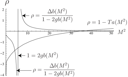
Figure 2: The graphs of the saddle-point equations by mathematica. We set $d=5$, and take $L=17$, $T=50$, $\Delta=12\pi^{2}$, and $g=18\pi^{2}$. The ordinate is $\rho\equiv\Delta b(M^{2})/[1-2gb(M^{2})]$, and the abscissa is $M^{2}$.

We find that there are two intersections at high temperature:

$$\rho^{*} \simeq \left\{\begin{array}[]{lr}\frac{\Delta b(M_{-}^{2*})}{1-2gb(M_{-}^{2*})}\equiv\rho_{-}^{*}&(M^{2}=M_{-}^{2*}),\\ 0\equiv\rho_{+}^{*}&(M^{2}={M_{+}^{2}}^{*}),\end{array}\right.$$ (102)

where ${M_{+}^{2}}^{*}>{M_{-}^{2}}^{*}$. Here, we compute the free energy densities at high temperature. Substituting the saddle point $i\lambda_{\alpha x}=m^{2}=M^{2}-\bar{Q}$ and $Q_{\alpha\beta x}=\bar{Q}$ into the replica partition function (III) and the action (85), we have the following expression for the free energy density $f$ ($\equiv F/V$) in the large $N$ limit:

$$f \simeq \frac{1}{2\beta}\biggl{[}\ln\biggl{(}\frac{\beta}{2\pi}\biggr{)}+\frac{1}{V}\sum_{k}\ln(-J\widehat{\Delta}_{k}+M^{2})\biggr{]}-Jd$$ (103)

$$-\frac{1}{2}M^{2}-\frac{\Delta+2g}{2}a(M^{2})+\frac{g}{2\beta}a(M^{2})^{2}.$$

As the temperature becomes higher, the intersections ${M_{-}^{2}}^{*}$ and ${M_{+}^{2}}^{*}$ become as follows:

$${M_{-}^{2}}^{*} = M_{0}^{2},$$ (104)

$${M_{+}^{2}}^{*} \simeq T,$$ (105)

where $M_{0}^{2}$ is given by solving the equation $1=2gb(M_{0}^{2})$. Thus, the free energy densities at high temperatures in both solutions are

$$f_{-} \equiv f(M_{-}^{2*}=M_{0}^{2})$$ (106)

$$\simeq \frac{1}{2\beta}\biggl{[}\ln\biggl{(}\frac{\beta}{2\pi}\biggr{)}+\frac{1}{V}\sum_{k}\ln(-J\widehat{\Delta}_{k}+M_{0}^{2})\biggr{]}-Jd$$

$$-\frac{1}{2}M_{0}^{2}-\frac{\Delta+2g}{2}a(M_{0}^{2})+\frac{g}{2\beta}a(M_{0}^{2})^{2},$$

$$f_{+} \equiv f(M_{+}^{2*}\simeq T)$$ (107)

$$\simeq -\frac{kT}{2}[1+\ln(2\pi)]-\frac{J^{2}d}{2kT}-\frac{\Delta+g}{2kT}.$$

The free energy density $f_{-}$ is lower than $f_{+}$. Performing the high temperature expansion without the replica method, however, we find that the result is consistent with $f_{+}$ in the leading order. Details of the calculation of the free energy density at the high temperature without the replica method are relegated to Appendix A. Thus, the solution $(M_{-}^{2*},\rho_{-}^{*})$ should be excluded. This choice of the solution $(M_{+}^{2*},\rho_{+}^{*})$ is consistent also with the result obtained by the functional renormalization group analysis in the large $N$ limit at zero temperature, as discussed in the final section. We also should note that the saddle point $(M_{+}^{2*},\rho_{+}^{*})$ exists in the region

$$1-2gb(M^{2})>0.$$ (108)

Near the critical point, $M$ becomes small, and then the field theoretical description is considered to be applicable. The integrals (94) and (95) can be expanded in $4<d<6$ as follows:

$$a(M^{2}) \simeq a_{0}-a_{1}M^{2},$$ (109)

$$b(M^{2}) \simeq b_{0}-b_{1}M^{d-4},$$ (110)

where $a_{0}$, $a_{1}$, $b_{0}$, and $b_{1}$ are the same positive constants as those of Eqs. (20) and (21). Inserting the above expansions into the saddle point equations (96) and (97), we get

$$1=kTa_{0}+(\Delta+2g)b_{0}-2g(kT)a_{0}(b_{0}-b_{1}M^{d-4}).$$ (111)

Putting $M=0$, we can get the critical line between ferromagnetic and paramagnetic phases:

$$kT_{c}a_{0}+(\Delta_{c}+2g)b_{0}-2g(kT_{c})a_{0}b_{0}=1,$$ (112)

$$(1-2gb_{0})\biggl{(}1-\frac{T_{c}}{T_{c}^{\rm(pure)}}\biggr{)}=\frac{\Delta_{c}}{\Delta_{c}^{(T=0)}}.$$ (113)

The phase diagram is depicted in Fig. 3.

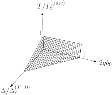
Figure 3: The phase diagram. The equation for the boundary surface is $(1-T_{c}/T_{c}^{\rm(pure)})(1-2gb_{0})=\Delta_{c}/\Delta_{c}^{(T=0)}$. The region containing the origin is the ferromagnetic phase. The other is paramagnetic.

We find that the ferromagnetic region is smaller than that in the absence of the random anisotropy term. As the strength of the random anisotropy increases, the ferromagnetic region becomes small. $M$ is rewritten by using $T_{c}$ and $\Delta_{c}$ as follows:

$$M = \biggl{\{}\biggl{[}\Delta+2g\biggl{(}1-\frac{T}{T_{c}^{\rm(pure)}}\biggr{)}\biggr{]}b_{1}\biggr{\}}^{-1/(d-4)}$$ (114)

$$\times\biggl{(}(1-2gb_{0})\frac{T-T_{c}}{T_{c}^{\rm(pure)}}+\frac{\Delta-\Delta_{c}}{\Delta_{c}^{(T=0)}}\biggr{)}^{1/(d-4)}.$$

Putting $\Delta=\Delta_{c}$, we have

$$M=\biggl{(}\frac{(1-2gb_{0})(T-T_{c})}{[\Delta_{c}T_{c}^{\rm(pure)}+2g(T_{c}^{\rm(pure)}-T)]b_{1}}\biggr{)}^{1/(d-4)}.$$ (115)

Putting $T=T_{c}$, we have

$$M=\biggl{(}\frac{(1-2gb_{0})(\Delta-\Delta_{c})}{[\Delta_{c}+(1-2gb_{0})(\Delta-\Delta_{c})]\Delta_{c}^{(T=0)}b_{1}}\biggr{)}^{1/(d-4)}.$$

Thus, the exponent $\nu$ of the correlation length is $\nu=1/2$.

III.2 Stability of replica-symmetric saddle point

We put

$$i\lambda_{\alpha x} = (M^{2}-\bar{Q})+i\epsilon_{\alpha x},$$ (117)

$$Q_{\alpha\beta x} = \bar{Q}+\eta_{\alpha\beta x},$$ (118)

$$\chi_{\alpha\beta x} = \bar{\chi}_{\alpha\beta}+\delta\chi_{\alpha\beta x}.$$ (119)

In the same way as in the previous section, we expand the effective action $S_{\rm eff}$ up to the second order of $\delta\chi_{\alpha\beta x}$. To study the stability of the saddle point against the off-diagonal fluctuations $\eta_{\alpha\beta k}$, we calculate the eigenvalue of the following Hessian:

$$G_{(\alpha\beta)(\gamma\delta)}\equiv\frac{\delta^{2}S_{\rm eff}}{\delta\eta_{\alpha\beta k}\delta\eta_{\gamma\delta,-k}}.$$ (120)

Putting the following ansatz (replicon subspace):

$$\epsilon_{\alpha}=\sum_{\gamma=1}^{n}\eta_{\alpha\gamma}=0,$$ (121)

we get the eigenvalue as

$$\lambda_{k} = \frac{1}{g}\biggl{(}1-2g\int_{q\in[-\pi,\pi]^{d}}\frac{d^{d}q}{(2\pi)^{d}}G_{0k-q}^{\rm C}G_{0q}^{\rm C}\biggr{)}$$ (122)

in the thermodynamic limit. Details of the calculation are shown in Appendix B. If the eigenvalue $\lambda_{k}$ is positive for all $k$, the saddle point is then stable against the off-diagonal fluctuations $\eta_{\alpha\beta k}$. First of all, putting $k=0$, we can easily investigate the eigenvalue

$$\lambda_{k=0} = \frac{1}{g}\biggl{(}1-2g\int_{q\in[-\pi,\pi]^{d}}\frac{d^{d}q}{(2\pi)^{d}}\frac{1}{(-J\widehat{\Delta}_{q}+M^{2})^{2}}\biggr{)}$$ (123)

$$= \frac{1}{g}[1-2gb(M^{2})].$$

The condition that the eigenvalue is positive is given by

$$1-2gb(M^{2})>0.$$ (124)

This is in agreement with the region (108) where the saddle point exists. Thus, the eigenvalue is positive in the region of the critical point and over. This result indicates that the replica-symmetric saddle point is stable against the fluctuation that is induced by introducing the second-rank random anisotropy, and therefore it is possible to integrate out the fluctuations $\eta_{\alpha\beta x}$. Even though we calculate the higher order corrections in $1/N$ expansion, we cannot find the instability of the replica-symmetric saddle point against the fluctuation. Therefore, the dimensional reduction holds for sufficiently large $N$.

IV Functional renormalization group for large $N$ models

We compare our results with the functional renormalization group (FRG) study at the zero temperature. Fi ; Fe ; Fe2 We search for a consistent FRG solution with the $1/N$ expansion. Details of the analysis are given in Appendix C. In general, a replicated Hamiltonian can be written as

$$\beta H_{\rm rep} = \frac{\beta}{2}\sum_{x}\sum_{\alpha}{\boldsymbol{S}}_{x,\alpha}\left(-J\hat{\Delta}_{x}\right){\boldsymbol{S}}_{x,\alpha}$$ (125)

$$-\frac{\beta^{2}}{2}\sum_{x}\sum_{\alpha,\beta}R\left({\boldsymbol{S}}_{x,\alpha}\cdot{\boldsymbol{S}}_{x,\beta}\right),$$

where the function $R(z)$ represents general anisotropy. Our Hamiltonian (74) corresponds to choosing

$$R(z)=\Delta z+gz^{2}.$$ (126)

First, we discuss the solutions in the large $N$ limit. If one takes the large $N$ limit, one finds exact solutions of all fixed points. We can analyze their stability by solving the eigenvalue equation of the infinitesimal deviation from the fixed-point solutions. This method is discussed by Balents and Fisher BF for random media. The one-loop beta function for a general $R(z)$ has both analytic and nonanalytic fixed points. Fi Following the method of Le Doussal and Wiese, DW we find one-parameter family of nonanalytic fixed points with a cusp. We obtain an asymptotic form of the solution near $z=1$,

$$R^{\prime}(z)\sim R^{\prime}(1)+\sqrt{2R^{\prime}(1)[\epsilon/A-R^{\prime}(1)](1-z)}.$$

Our analysis shows that all physical nonanalytic fixed points satisfying the Schwartz-Soffer inequalitySS have many unstable modes.

In addition to the nonanalytic fixed points, we find four analytic fixed points given in Eq. (126) with $(\Delta,g)=(0,0),(\epsilon/A,0),(0,\epsilon/(2A))$, and $(-\epsilon/A,\epsilon/(2A))$, where $\epsilon=d-4$. The last one is unphysical since $\Delta<0$. The triangle defined by the other three fixed points corresponds to ferromagnetic region on the $T=0$ plane in Fig. 3. In fact, the vertex $(\Delta,g)=(\Delta_{c}^{(T=0)},0)=(1/b_{0},0)$ corresponds to (113) with $T_{c}=0$. It is easily seen that

$$\frac{1}{b_{0}}=\frac{\epsilon}{A}\Lambda^{-\epsilon},$$ (127)

where $\Lambda$ is a momentum cutoff. Thus the dimensionless quantity $(\Delta,g)\Lambda^{\epsilon}$ is equal to the analytic fixed point $(\epsilon/A,0)$. Similarly, the vertex $(0,1/(2b_{0}))$ corresponds to the fixed point $(0,\epsilon/(2A))$. Therefore, we find that the phase diagram at $T=0$ obtained by the large $N$ limit is understood by the functional renormalization group method. Furthermore, the stability analysis in Appendix C shows that $(\epsilon/A,0)$ is singly unstable, where the unstable mode corresponds to deformation along $\Delta$ axis. The origin $(0,0)$ is fully stable while $(0,\epsilon/(2A))$ is fully unstable. Therefore, in the large $N$ limit, a phase transition at $T=0$ is governed by the singly unstable fixed point $(\epsilon/A,0)$ yielding dimensional reduction. The corresponding flow in the two dimensional coupling constant space is depicted in Fig. 4.

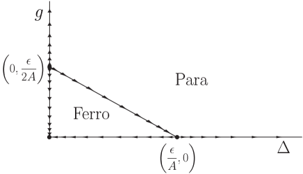
Figure 4: The renormalization group flow for the couplings $\Delta$ and $g$ in the large $N$ limit.

Next, we discuss the model with a finite $N$. We conclude that the dimensional reduction holds for sufficiently large $N$. We study the singly unstable analytic fixed point found in the large $N$ limit. By the discussion in Appendix C, the fixed point to control the phase transition has

$$R^{\prime}(1)=\frac{d-4}{A(N-2)}\ \ \ \ {\rm or}\ \ \ \ 0.$$

At this stage, we find only two possibilities. The exponents of the correlation function becomes those given by the dimensional reduction

$$\eta=\bar{\eta}=\frac{d-4}{N-2}.$$ (128)

or the trivial ones

$$\eta=\bar{\eta}=0.$$ (129)

We obtain the subleading correction to this fixed point solution

$$R(z)=\frac{\epsilon}{A}\left[z-\frac{1}{2}+\frac{1}{2N}(z^{2}+2z)+{\rm O}\left(\frac{1}{N^{2}}\right)\right].$$ (130)

We analyze the stability of this analytic fixed point yielding the dimensional reduction by solving the eigenvalue equation of the linearized beta function in Appendix C. There are many unphysical modes which diverge in the interval $-1\leq z\leq 1$. These are not generated in the flow, thus we eliminate these unphysical modes by choosing the integral constants. These unphysical modes correspond to the infinitely many relevant modes pointed out by Fisher. Fi In our solution of the eigenvalue equation, we find the same eigenvalues calculated by Fisher up to the order $1/N$, if we correct an expression given there by adding an overlooked term. We discuss this problem in Appendix C. The analytic fixed point $(\epsilon/A,0)$ has slightly relevant operators with dimension less than $2/N$, which give deformation of the coupling $\delta R^{\prime}(z)\sim(1-z)^{-\alpha}$ with $0<-\alpha<2/N$. Here, we discuss this subtle problem of the slightly relevant operators. First, we assume that the initial coupling constant $R^{\prime\prime}(1)$ in the renormalization group equation is finite. In this case, this fixed point behaves as a singly unstable fixed point in the following reason. By Fisher’s representation of the renormalization group equation, $R^{\prime}(1)$ and $R^{\prime\prime}(1)$ satisfy

$$\partial_{t}R^{\prime}(1)\!\!\! = \!\!\!(4-d)R^{\prime}(1)+A(N-2)R^{\prime}(1)^{2},$$

$$\partial_{t}R^{\prime\prime}(1)\!\!\! = \!\!\!(4-d)R^{\prime\prime}(1)+A(6R^{\prime}(1)R^{\prime\prime}(1)$$ (131)

$$+(N+7)R^{\prime\prime}(1)^{2}+R^{\prime}(1)^{2}).$$

For a small initial value of $R^{\prime\prime}(1)$ the flow of $R^{\prime\prime}(1)$ stays in a compact area. The flow in the two-dimensional coupling constant space is qualitatively the same as in Fig. 4.

In this case, if $R^{\prime}(1)$ takes a critical value by tuning the coupling constant $\Delta$ or $g$, the coupling $R(z)$ flows toward the analytic fixed point with a finite $R^{\prime\prime}(1)$. Then, the flow does not generate the relevant mode with an exponent $0<-\alpha<2/N$ from an initial function with a finite $R^{\prime\prime}(1)$. This analytic fixed point controls the phase transition, and therefore the critical behavior obeys the dimensional reduction. Since this analytic fixed point exists for $N\geq 18$ as pointed out by Fisher, Fi the dimensional reduction occurs for $N\geq 18$. In this case, the critical exponents of correlation function are given by (128). This result agrees with our simple $1/N$ expansion. Next, we consider that the initial coupling constant $R^{\prime\prime}(1)$ is not finite. We assume

$$R^{\prime}(z)=C(1-z)^{-\alpha},$$

with $0<-\alpha<1$. Since $R^{\prime\prime}(1)$ diverges, already at the initial stage the coupling constants are infinitely far from the analytic fixed points for any small $C$. We cannot justify whether or not the continuum field theory approximation induces such a mode in the initial function. Theoretically, however, we can consider such a model. The renormalization group transformation can generate a term proportional to $(1-z)^{-2\alpha-1}.$ Since $-2\alpha-1<-\alpha$, the successive transformation may produce less power. Eventually, the flow generates a relevant mode with $-\alpha<2/N$ and the flow cannot reach the analytic fixed point by tuning the parameter $\Delta$ and $g$. Since all fixed points are unstable except the trivial one, the flow reaches the trivial fixed point directly in the massless phase. In this case, we obtain only trivial critical exponents (129). This second possibility does not agree with our $1/N$-expansion method. Therefore, only consistent result with the $1/N$ expansion is the dimensional reduction.

V Discussion and summary

In this paper, we have studied the random field O($N$) spin model including the second-rank random anisotropy term. We have studied the effect of the second-rank random anisotropy on the critical phenomena of the random field O($N$) spin model in $4<d<6$, by use of the replica method and the $1/N$-expansion method. The off-diagonal fluctuations are induced through the Hubbard-Stratonovich transformation for the second-rank random anisotropy. We have computed the saddle point under the assumption of the replica symmetry, and have studied the stability of the replica symmetric saddle point against the off-diagonal fluctuations which are induced by the second-rank random anisotropy. Our criterion to judge the stability of the system is identical to the standard one used by de Almeida and Thouless. AT It is based on the stability of the saddle point of the auxiliary field introduced to calculate the partition function explicitly. We find that the eigenvalues of the Hessian around the replica symmetric saddle point are positive definite, and thus the Gaussian integration over auxiliary field can be performed. The instability is not observed in higher order correction in the $1/N$ expansion. Consequently, we conclude that the replica-symmetric saddle point is stable for a second-rank random anisotropy with the order $1/N$ and the dimensional reduction holds for sufficiently large $N$.

This result is inconsistent with that obtained by Mézard and Young. MY Since the SCSA equation gives the precise two-point correlation function up to order $1/N$, their replica-symmetric two-point correlation function agrees with ours. Nonetheless, they conclude that the replica-symmetric correlation function is unstable against a deviation of the correlation function by treating the free energy as a functional of two point correlation function. Their criterion for stability differs from the de Almeida-Thouless one, although it looks the same. They optimize the free energy by choosing the two-point correlation function freely. On the other hand, in our analysis, a two-point correlation function can be deformed only through changing a saddle point of the auxiliary field, and then it cannot be deformed freely. This is the essential difference between two theories. We consider either that the instability shown by Mézard and Young MY is just apparent, or that their method includes some nonperturbative effects other than the $1/N$ expansion. For the latter possibility, we should justify that the free energy can be optimized by a correlation function with no constraint.

We have checked the consistency between the large $N$ analysis and the renormalization group flow by showing that the phase boundaries obtained in those methods are consistent in $4+\epsilon$ dimensions. As pointed by Feldman, Fe the critical phenomena near the lower critical dimension is governed by the nonanalytic fixed point by the appearance of the cusp, and then the dimensional reduction breaks down for some small $N$. For large $N$, however, we show that the functional renormalization group method studied by Feldman allows us to perform the $1/N$ expansion. We find all fixed points which consist of analytic and nonanalytic ones in the large $N$ limit. On the other hand for $N<18$, it is known that there are no nontrivial analytic fixed points. Fi By solving the eigenvalue problem for the infinitesimal deviation from the fixed point, we find that the nonanalytic fixed points are fully unstable. We search for consistent solutions of the renormalization group with the $1/N$ expansion. If the initial $R^{\prime\prime}(1)$ is finite, the nonanalytic relevant modes cannot be generated. In this case, the unique analytic fixed point practically behaves as a singly unstable fixed point, which gives the dimensional reduction. This result agrees with the stability of the replica-symmetric saddle-point solution in the $1/N$ expansion. Thus, we conclude dimensional reduction occurs.

Our result also agrees with a recent study of the random field O($N$) model by Tarjus and Tissier. They study the model by a nonperturbative functional renormalization group. TT Although their work to obtain a full solution is in progress, they give a global picture in a $d$-$N$ phase diagram and discuss the consistency of their results with those by some perturbative results. They propose a scheme to fix a phase boundary of the phase where the dimensional reduction breaks down. Using an approximation method, they show that the phase is in a compact area on the $d$-$N$ plane.

Here, we comment on the model in dimension less than $4$. The $1/N$-expansion method shows that the model has a massive paramagnetic phase only. Also, the functional renormalization group method for negative $\epsilon=d-4$ shows that there are no nontrivial analytic fixed points. The trivial fixed point and nonanalytic fixed points are unstable for $d<4$. Our large $N$ analysis indicates that the nonanalytic fixed points are unstable, and therefore only a massive phase exists. This result agrees with Feldman’s result Fe2 that the correlation length is finite always for $N\geq 10$.

Finally, we comment on the critical behavior near the upper critical dimensions. In a recent work, MS the dimensional reduction has been shown by a perturbative renormalization group in a coupling constant space near the upper critical dimension in the random field Ising model at one-loop order. This result is also consistent with that obtained by Tarjus and Tissier. TT This study can be extended to the ${\rm O}(N)$ model and the result agrees with the $1/N$ expansion. These studies suggest that the large $N$ limit may be applicable to the model with a small $N$ near the upper critical dimensions. However, it is a nontrivial problem whether or not the dimensional reduction holds near the upper critical dimension for a small $N$. Further studies are needed.

Appendix A Free energy at high temperature without replica method

The Hamiltonian is given by

$$H = -J\sum_{\langle x,y\rangle}{\mbox{\boldmath$S$}}_{x}\cdot{\mbox{\boldmath$S$}}_{y}-\sum_{x}{\mbox{\boldmath$h$}}_{x}\cdot{\mbox{\boldmath$S$}}_{x}-\sum_{x}({\mbox{\boldmath$h$}}_{x}\cdot{\mbox{\boldmath$S$}}_{x})^{2}$$ (132)

$$= -J\sum_{\langle x,y\rangle}\sum_{i=1}^{N}S_{x}^{(i)}S_{y}^{(i)}-\sum_{x}\sum_{i=1}^{N}h_{x}^{(i)}S_{x}^{(i)}$$

$$-\sum_{x}\sum_{i,j}^{N}h_{x}^{(i)}h_{x}^{(j)}S_{x}^{(i)}S_{x}^{(j)}$$

$$= -J\sum_{\langle x,y\rangle}\sum_{i=1}^{N}S_{x}^{(i)}S_{y}^{(i)}-\sum_{x}\sum_{i=1}^{N}h_{x}^{(i)}S_{x}^{(i)}$$

$$-\sum_{x}\sum_{i,j}^{N}h_{2,x}^{(ij)}S_{x}^{(i)}S_{x}^{(j)}.$$

Here, $h_{x}^{(i)}$ and $h_{2,x}^{(ij)}$ are the random field and the second-rank random anisotropy, respectively:

$$\!\!\!\!\!\![h_{x}^{(i)}]=0,\quad[h_{x}^{(i)}h_{y}^{(j)}]=\Delta\delta_{ij}\delta_{xy},$$ (133)

$$\!\!\!\!\!\![h_{2,x}^{(ij)}]=0,\,[h_{2,x}^{(ij)}h_{2,y}^{(kl)}]=\frac{g}{2}(\delta_{ik}\delta_{jl}+\delta_{il}\delta_{jk})\delta_{xy}.$$ (134)

The partition function is

$$Z=\biggl{(}\prod_{x}\int_{-\infty}^{\infty}d{\mbox{\boldmath$S$}}_{x}\delta({{\mbox{\boldmath$S$}}_{x}}^{2}-1)\biggr{)}e^{-\beta H}.$$ (135)

Here we put

$$\prod_{x}\int_{-\infty}^{\infty}d{\mbox{\boldmath$S$}}_{x}\delta({\mbox{\boldmath$S$}}_{x}^{2}-1)=\int{\cal{D}}{\mbox{\boldmath$S$}}$$ (136)

Performing the calculation of the measure $\int{\cal{D}}{\mbox{\boldmath$S$}}$, we have

$$\int{\cal{D}}{\mbox{\boldmath$S$}}1=\prod_{x}\frac{N\pi^{N/2}}{2\Gamma(\frac{N}{2}+1)}\simeq\exp[Vs(N)],$$ (137)

$$s(N) \simeq \frac{N}{2}[1+\ln(2\pi)],$$ (138)

for $N\gg 1$.

We study the behavior of the free energy at high temperatures. We expand the partition function in $\beta H$ up to the second order:

$$Z = \int{\cal{D}}{\mbox{\boldmath$S$}}e^{-\beta H}$$ (139)

$$\simeq e^{Vs(N)}\biggl{(}1-\langle\beta H\rangle+\frac{1}{2!}\langle(\beta H)^{2}\rangle\biggr{)},$$

where the angular brackets $\langle\cdots\rangle$ stand for

$$\langle f({\mbox{\boldmath$S$}})\rangle\equiv\frac{\int{\cal{D}}{\mbox{\boldmath$S$}}f({\mbox{\boldmath$S$}})}{\int{\cal{D}}{\mbox{\boldmath$S$}}1}=e^{-Vs(N)}\int{\cal{D}}{\mbox{\boldmath$S$}}f({\mbox{\boldmath$S$}}).$$ (140)

Then, $\ln Z$ is

$$\ln Z \simeq Vs(N)-\langle\beta H\rangle+\frac{1}{2}\langle\beta H;\beta H\rangle,$$ (141)

where

$$\langle\beta H;\beta H\rangle\equiv\langle(\beta H)^{2}\rangle-\langle\beta H\rangle^{2}.$$ (142)

Using the identity $\langle S_{x}^{(i)}S_{y}^{(j)}\rangle=\delta_{xy}\delta_{ij}$, and Eqs. (133) and (134), we have

$$f\!\!\! = \!\!\!-\frac{1}{\beta}[\ln Z]$$

$$\simeq \!\!\!-\frac{NkT}{2}[1+\ln(2\pi)]-\frac{J^{2}d}{2NkT}-\frac{N\Delta+Ng}{2NkT}.$$

According to the redefinition of the parameters (83), the free energy density is rewritten as

$$f = -\frac{1}{\beta}[\ln Z]$$ (144)

$$\simeq -\frac{kT}{2}[1+\ln(2\pi)]-\frac{J^{2}d}{2kT}-\frac{\Delta+g}{2kT}.$$

This is in agreement with Eq. (107).

Appendix B Derivation of eigenvalue (122)

In this appendix, we give the details of the calculation of the eigenvalue (122).

The second-order term of $\delta\chi_{\alpha\beta x}$ and $\eta_{\alpha\beta x}$ for the effective action $S_{\rm eff}$ becomes

$$\delta^{2}S_{\rm eff}\!\!\! = \!\!\!-\frac{N}{4}\int d^{d}x$$ (145)

$$\!\!\!\!\!\!\times\biggl{\langle}x\biggr{|}{\rm Tr}\frac{1}{-J\widehat{\Delta}_{x}{\mbox{\boldmath$1$}}_{n}+{\mbox{\boldmath$\bar{\chi}$}}}\delta{\mbox{\boldmath$\chi$}}\frac{1}{-J\widehat{\Delta}_{x}{\mbox{\boldmath$1$}}_{n}+{\mbox{\boldmath$\bar{\chi}$}}}\delta{\mbox{\boldmath$\chi$}}\biggl{|}x\biggr{\rangle}$$

$$\!\!\!\!\!\!+\frac{N}{8g}\int d^{d}x\sum_{\alpha\neq\beta}^{n}\eta_{\alpha\beta x}^{2}.$$

In the momentum representation, the second-order correction of the action $S_{\rm eff}$ is rewritten as

$$\delta^{2}S_{\rm eff}\!\!\! = \!\!\!\frac{N}{4}\int_{k\in[-\pi,\pi]^{d}}\frac{d^{d}k}{(2\pi)^{d}}\biggl{(}\sum_{\alpha,\gamma}^{n}\epsilon_{\alpha k}\epsilon_{\gamma,-k}G_{\alpha\gamma}$$ (146)

$$+2\sum_{\alpha=1}^{n}\sum_{\gamma<\delta}\epsilon_{\alpha k}\eta_{\gamma\delta,-k}G_{\alpha(\gamma\delta)}$$

$$+\sum_{\alpha<\beta}\sum_{\gamma<\delta}\eta_{\alpha\beta k}\eta_{\gamma\delta,-k}G_{(\alpha\beta)(\gamma\delta)}\biggr{)}.$$

Here

$$G_{\alpha\alpha}\!\!\! = \!\!\!G_{0}^{\alpha\alpha}*G_{0}^{\alpha\alpha}\equiv{\cal{A}},$$ (147)

$$G_{\alpha\gamma}\!\!\! = \!\!\!G_{0}^{\alpha\gamma}*G_{0}^{\gamma\alpha}\equiv{\cal{B}}\quad(\alpha\neq\gamma),$$ (148)

$$G_{\alpha(\alpha\delta)}\!\!\! = \!\!\!\frac{i}{2}(G_{0}^{\alpha\alpha}*G_{0}^{\delta\alpha}+G_{0}^{\delta\alpha}*G_{0}^{\alpha\alpha}$$ (149)

$$+G_{0}^{\alpha\delta}*G_{0}^{\alpha\alpha}+G_{0}^{\alpha\alpha}*G_{0}^{\alpha\delta})$$

$$\equiv \!\!\!{\cal{C}}\quad(\alpha\neq\delta),$$

$$G_{\alpha(\gamma\delta)}\!\!\! = \!\!\!\frac{i}{2}(G_{0}^{\alpha\gamma}*G_{0}^{\delta\alpha}+G_{0}^{\delta\alpha}*G_{0}^{\alpha\gamma}$$ (150)

$$+G_{0}^{\alpha\delta}*G_{0}^{\gamma\alpha}+G_{0}^{\gamma\alpha}*G_{0}^{\alpha\delta})$$

$$\equiv \!\!\!{\cal{D}}\quad(\alpha\neq\gamma,\delta,\,\gamma\neq\delta),$$

$$G_{(\alpha\beta)(\alpha\beta)}\!\!\! = \!\!\!\frac{1}{Ng}-(G_{0}^{\beta\alpha}*G_{0}^{\beta\alpha}+G_{0}^{\alpha\alpha}*G_{0}^{\beta\beta}$$ (151)

$$+G_{0}^{\beta\beta}*G_{0}^{\alpha\alpha}+G_{0}^{\alpha\beta}*G_{0}^{\alpha\beta})$$

$$\equiv \!\!\!{\cal{P}}\quad(\alpha\neq\beta),$$

$$G_{(\alpha\beta)(\alpha\delta)}\!\!\! = \!\!\!-(G_{0}^{\beta\alpha}*G_{0}^{\delta\alpha}+G_{0}^{\alpha\alpha}*G_{0}^{\delta\beta}$$ (152)

$$+G_{0}^{\beta\delta}*G_{0}^{\alpha\alpha}+G_{0}^{\alpha\delta}*G_{0}^{\alpha\beta})$$

$$\equiv \!\!\!{\cal{Q}}\quad(\alpha\neq\beta,\delta,\,\beta\neq\delta),$$

$$G_{(\alpha\beta)(\gamma\delta)}\!\!\! = \!\!\!-(G_{0}^{\beta\gamma}*G_{0}^{\delta\alpha}+G_{0}^{\alpha\gamma}*G_{0}^{\delta\beta}$$ (153)

$$+G_{0}^{\beta\delta}*G_{0}^{\gamma\alpha}+G_{0}^{\alpha\delta}*G_{0}^{\gamma\beta})$$

$$\equiv \!\!\!{\cal{R}}\quad(\alpha\neq\beta,\gamma,\delta,\,\beta\neq\gamma,\delta\,\gamma\neq\delta).$$

$$G_{0}^{\alpha\beta}*G_{0}^{\gamma\delta}=\int_{q\in[-\pi,\pi]^{d}}\frac{d^{d}q}{(2\pi)^{d}}G_{0k-q}^{\alpha\beta}G_{0q}^{\gamma\delta}.$$ (154)

We shall find the eigenvalues of the matrix $G$ (Hessian)

$$G=\left(\begin{array}[]{cc}\{G_{\alpha\gamma}\}&\{G_{\alpha(\gamma\delta)}\}\\ \{G_{(\alpha\beta)\gamma}\}&\{G_{(\alpha\beta)(\gamma\delta)}\}\end{array}\right).$$ (157)

Let $\vec{\mu}$ be the eigenvector associated with the eigenvalue $\lambda$;

$$\vec{\mu}=\left(\begin{array}[]{c}\{\epsilon_{\gamma}\}\\ \{\eta_{\gamma\delta}\}\\ \end{array}\right),$$ (160)

where $\eta_{\gamma\delta}=\eta_{\delta\gamma}$. Applying $G$ to $\vec{\mu}$, we obtain

$$(G\vec{\mu})_{\alpha} = {\cal A}\epsilon_{\alpha}+{\cal B}\sum_{\gamma\neq\alpha}^{n}\epsilon_{\gamma}+{\cal C}\sum_{\gamma\neq\alpha}^{n}\eta_{\alpha\gamma}$$ (161)

$$+\frac{{\cal D}}{2}\sum_{\gamma\neq\alpha}^{n}\sum_{\delta\neq\gamma,\alpha}^{n}\eta_{\gamma\delta},$$

$$(G\vec{\mu})_{\alpha\beta} = {\cal C}(\epsilon_{\alpha}+\epsilon_{\beta})+{\cal D}\sum_{\gamma\neq\alpha,\beta}^{n}\epsilon_{\gamma}+{\cal P}\eta_{\alpha\beta}$$

$$+2{\cal Q}\sum_{\gamma\neq\alpha,\beta}^{n}\eta_{\alpha\gamma}+\frac{{\cal R}}{2}\sum_{\gamma\neq\alpha,\beta}^{n}\sum_{\delta\neq\gamma,\alpha,\beta}^{n}\eta_{\gamma\delta}.$$

To find the solution of Eqs. (161) and (B), we use the following ansatz according to Ref. MY, :

$$\epsilon_{\alpha}=\sum_{\gamma=1}^{n}\eta_{\alpha\gamma}=0$$ (163)

for all $\alpha$. Under this ansatz, Eq. (B) gives a nontrivial solution

$$(G\vec{\mu})_{\alpha\beta}=({\cal P}-2{\cal Q}+{\cal R})\eta_{\alpha\beta}=\lambda\eta_{\alpha\beta}.$$ (164)

Therefore, we get the eigenvalue (122).

Appendix C Functional renormalization group study for critical phenomena of random field O($N$) spin model in $4+\epsilon$ dimensions

In this appendix we study the one-loop beta function derived by Fisher Fi for a general random disorder $R(z)$ at zero temperature:

$$\partial_{t}R(z)\!\!\! = \!\!\!(4-d)R(z)+A\biggl{(}2(N-2)R^{\prime}(1)R(z)$$ (165)

$$\!\!\!\!\!\!-(N-1)zR^{\prime}(1)R^{\prime}(z)+(1-z^{2})R^{\prime}(1)R^{\prime\prime}(z)$$

$$\!\!\!\!\!\!+\frac{1}{2}[R^{\prime}(z)]^{2}(N-2+z^{2})-R^{\prime}(z)R^{\prime\prime}(z)z(1-z^{2})$$

$$\!\!\!\!\!\!+\frac{1}{2}[R^{\prime\prime}(z)]^{2}(1-z^{2})^{2}\biggr{)}.$$

Here, $t=\ln l$ with $l$ being the length scale specifying the FRG and $A=S_{d}/(2\pi)^{d}J^{2}$.

C.1 General properties of fixed points

The fixed point condition of the renormalization group determines properties of the function $R(z)$. Here we discuss possible asymptotic behaviors of $R(z)$ near $z=1$. The first derivative of the fixed point equation with respect to $z$ is

$$[(4-d)/A+(N-1)]R^{\prime}(1)R^{\prime}(z)+zR^{\prime}(z)^{2}$$

$$-(N+1)zR^{\prime}(1)R^{\prime\prime}(z)+(N-2+3z^{2})R^{\prime}(z)R^{\prime\prime}(z)$$

$$+(1-z^{2})R^{\prime}(1)R^{\prime\prime\prime}(z)-z(1-z^{2})R^{\prime}(z)R^{\prime\prime\prime}(z)$$

$$-3z(1-z^{2})R^{\prime\prime}(z)^{2}+(1-z^{2})^{2}R^{\prime\prime}(z)R^{\prime\prime\prime}(z)$$

$$-(1-z^{2})R^{\prime}(z)R^{\prime\prime}(z)=0.$$ (166)

If we assume asymptotic behavior of $R^{\prime}(z)$ near $z=1$,

$$R^{\prime}(z)=R^{\prime}(1)+C(1-z)^{\gamma}+\cdots,$$ (167)

with $0<\gamma$. To discuss a cuspy behavior of $R(z)$ at $z=1$, we consider only $\gamma<1$. The condition (166) gives the following constraint:

$$[(4-d)/A+(N-2)R^{\prime}(1)]R^{\prime}(1)$$

$$-C^{2}\gamma(4\gamma^{2}+4\gamma+N-1)(1-z)^{2\gamma-1}=0.$$ (168)

For $\gamma\neq 1/2$, this constraint gives

$$\gamma=\frac{1}{2}(-1+\sqrt{2-N})\ \ \ \ {\rm or}\ \ \ \ C=0,$$

and also

$$R^{\prime}(1)=\frac{d-4}{A(N-2)}\ \ \ \ {\rm or}\ \ \ \ R^{\prime}(1)=0.$$

Here, the former case shows the dimensional reduction. The formulas for the critical exponents obtained by Feldman, Fe

$$\eta=AR^{\prime}(1),\ \ \ \ \bar{\eta}=A(N-1)R^{\prime}(1)-\epsilon,$$ (169)

enable us to obtain

$$\eta=\frac{d-4}{N-2}=\bar{\eta}.$$ (170)

In this case, no $\gamma$ is allowed for any $N$. For $\gamma=1/2$, the parameter $R^{\prime}(1)$ can change continuously depending on the constant $C$. Therefore, only $\gamma=1/2$ allows divergent $R^{\prime\prime}(1)$. Only this case does the nontrivial critical behavior differ from the dimensional reduction. Since the initial value $R(z)$ of the renormalization group equation (165) is an analytic function, the flow of $R^{\prime\prime}(1)$ should diverge for the breakdown of the dimensional reduction.

The same discussion for $z=-1$ can be done. The only possible singularity is

$$R^{\prime}(z)=R^{\prime}(-1)+C(1+z)^{1/2}+\cdots.$$

If $C=0$, then we have

$$R^{\prime}(-1)=(N-3)R^{\prime}(1)-\frac{d-4}{A}\ \ \ \ {\rm or}\ \ \ \ R^{\prime}(-1)=0.$$

C.2 Large-$N$ limit

In order to take the large $N$ limit, we multiply both sides by $N$ and rescale $NR\rightarrow R$. The beta function becomes

$$\partial_{t}R(z)\!\!\! = \!\!\!(4-d)R(z)+A\biggl{(}2R^{\prime}(1)R(z)-zR^{\prime}(1)R^{\prime}(z)$$ (171)

$$+\frac{1}{2}[R^{\prime}(z)]^{2}\biggr{)}+{\rm O}(1/N).$$

C.3 Fixed points

Following the method given by Balents and Fisher, BF we consider the flow equation for $R^{\prime}(z)$ instead of that for $R(z)$. Taking the derivative with respect to $z$ and introducing $u(z)$ defined by

$$R^{\prime}(z)\equiv\frac{\epsilon}{A}u(z),$$ (172)

the fixed point equation for (171) becomes

$$(a-1)u(z)-zau^{\prime}(z)+u(z)u^{\prime}(z)=0$$ (173)

in the large $N$ limit. Here we define $a=u(1)$. First we solve it when $a=1$. In this case, $u(z)$ satisfies $u^{\prime}(z)\equiv 0$ or $u(z)=z$. If $u^{\prime}(z)=0$ then $u(z)=1$ since $a=u(1)=1$. Thus

$$R(z)=\frac{\epsilon}{A}\biggl{(}z-\frac{1}{2}\biggr{)},$$ (174)

where the constant term $-\epsilon/(2A)$ is determined by (171). On the other hand, in the case of $u(z)=z$,

$$R(z)=\frac{\epsilon}{2A}z^{2}.$$ (175)

Next, we turn to the case of $a=0$, where $u(z)$ satisfies $u(z)\equiv 0$ or $u^{\prime}(z)=1$. The former case is $R(z)=0$, which corresponds to the pure theory. The latter becomes

$$u(z)=(z-1);$$ (176)

namely,

$$R(z)=\frac{\epsilon}{2A}\left(z-1\right)^{2}.$$ (177)

Those analytic fixed points were first obtained by Feldman. Fe2

Next we consider a general case. If $a\neq 0,1$,

$$\frac{du}{dz}=\frac{(a-1)u}{za-u}.$$ (178)

Taking the inversion we regard $z$ as a function of $u$. DW One gets

$$\frac{dz}{du}=\frac{a}{a-1}\frac{z}{u}-\frac{1}{a-1},$$ (179)

which is easily integrated The result is

$$z(u)=C\left|u\right|^{a/(a-1)}+u,$$ (180)

where $C$ is a constant. Since $z(u)$ satisfies $z(a)=1$, $C$ is determined uniquely as

$$z(u)=(1-a)\biggl{(}\frac{u}{a}\biggr{)}^{a/(a-1)}+u.$$ (181)

Now we revert (181) to the solution $u(z)$ for (178). Because $z(u)$ takes the maximum value 1 at $u=a$, $u(z)$ is double valued as we show in Fig. 5. It is seen from (178) that $du/dz$ is ill defined on $u=az$. Therefore the lower branch terminates at the origin, so that it should be continued to the region $-1\leq z<0$. This is possible only if $a/(a-1)$ is a positive integer.

Figure 5: A schematic graph of $u(z)$. Since the derivative of $u$ is ill defined on $u=az$, the solution terminates on this line. The above graph represents two solutions meeting at $(1,a)$.

Nonanalytic behavior near $z=1$ is clarified as follows. Set

$$u=a+\delta u$$ (182)

and assume that $\left|\delta u\right|\ll|a|$. From (181),

$$u(z)=a\pm\sqrt{2a(a-1)(1-z)}+\cdots.$$ (183)

Note that the plus (minus) sign in front of the square root means to take the upper (lower) branch. Nonanalytic behavior is seen at $z=1$. Since the function $u(z)$ should be real in $|z|\leq 1$, $a$ satisfies $a(a-1)\geq 0$. Furthermore, ${\bar{\eta}}=\epsilon a/N$ should be nonnegative due to physical requirements [see (169)]; hence

$$a>1.$$ (184)

C.4 Stability of the fixed points

Next we investigate the stability of the solutions. Let $u^{*}$ be a fixed point solution:

$$(a-1)u^{*}-za{u^{*}}^{\prime}+u^{*}{u^{*}}^{\prime}=0.$$ (185)

To study the stability of $u^{*}$, let $u=u^{*}+v$. Inserting this into (173) and keeping up to the linear terms of $v$, we consider the following eigenvalue problem:

$$[(a-1)+u^{\prime}]v+(u-za)v^{\prime}+(u-zu^{\prime})v(1)=\lambda v.$$ (186)

Here we omit the asterisk from $u^{*}$ for brevity. Normalizing $v$ appropriately, we can take $v(1)=0$ or $v(1)=1$. We begin with the analytic cases.

C.4.1 $R(z)=\epsilon(z-1/2)/A$

In this case, $a=1$ and $u(z)\equiv 1$. Then (186) becomes

$$(1-z)v^{\prime}+b=\lambda v,$$ (187)

where $b$ represents $v(1)$ taking 0 or 1. When $b=0$ the solution is

$$v(z)=C(1-z)^{-\lambda},$$ (188)

where $\lambda<0$ because of the initial condition $b=v(1)=0$. On the other hand, when $b=1$, a general solution is

$$v(z)=\left\{\begin{array}[]{ll}\lambda^{-1}+c(1-z)^{-\lambda}&(\lambda\neq 0),\\ \ln|1-z|&(\lambda=0).\end{array}\right.$$ (189)

Here the condition $b=1$ requires that $\lambda=1$ and $c=0$. In conclusion, the allowed value of $\lambda$ is $\lambda<0$ or $\lambda=1$. This shows that the fixed point solution is singly unstable.

C.4.2 $R(z)=\epsilon z^{2}/(2A)$

In this case, $a=1$ and $u=z$; hence (186) is simplified to $v=\lambda v$ for $b=0,1$. It means that $\lambda=1$ for every deformation, so that this fixed point is fully unstable. This is also true for any finite $N$.

C.4.3 $R=0$

Since $a=0$ and $u=0$ in this case, (186) is $-v=\lambda v$, which means $\lambda=-1$ for any $v$; thus the trivial fixed point is fully stable.

C.4.4 $R(z)=\epsilon(z-1)^{2}/(2A)$

Here, $a=0$ and $u=z-1$. The eigenvalue equation is

$$-(1-z)v^{\prime}-b=\lambda v,$$ (190)

which can be solved in a similar way as for (187). The result is

$$v(z)=C(1-z)^{\lambda}$$ (191)

for $b=0$ and

$$v(z)=\left\{\begin{array}[]{ll}-\lambda^{-1}+c(1-z)^{\lambda}&(\lambda\neq 0),\\ \ln|1-z|&(\lambda=0)\end{array}\right.$$ (192)

for $b=1$. Therefore the allowed values of $\lambda$ are

$$\lambda>0\ \ {\mbox{and}}\ \ \lambda=1.$$ (193)

Therefore it is unstable.

C.4.5 Nonanalytic case

Next we proceed to the nonanalytic case. Using (178), we regard $v$ as function of $u$. Then (186) is written as

$$\frac{dv}{du}+f(u)v+g(u)b=0,$$ (194)

where

$$f(u) = \left(\frac{\lambda}{a-1}-1\right)\frac{1}{u}-\frac{1}{az-u},$$

$$g(u) = \frac{z-u}{(1-a)(za-u)}.$$ (195)

A general solution of (194) is

$$v=\left\{\begin{array}[]{ll}Ce^{-F(u)}&(b=0),\\ -e^{-F(u)}\int e^{F(u)}g(u)du&(b=1),\end{array}\right.$$ (196)

where

$$F(u)\equiv\int f(u)du.$$ (197)

Let us compute $F(u)$. Since $z$ is given as a function of $u$ by (181), we can write

$$\int\frac{du}{az-u} = \int\frac{d\hat{u}}{1-a}\left(\frac{\hat{u}^{1/(a-1)-1}}{\hat{u}^{1/(a-1)}-1}-\frac{1}{\hat{u}}\right),$$ (198)

where

$$\hat{u}\equiv\frac{u}{a}.$$ (199)

Thus, using the ambiguity of the constant term of $F(u)$, we get

$$F(u)=\frac{\lambda-a}{a-1}\ln\hat{u}+\ln|1-\hat{u}^{1/(a-1)}|.$$ (200)

Therefore,

$$e^{-F(u)}=\hat{u}^{(a-\lambda)/(a-1)}|1-\hat{u}^{1/(a-1)}|^{-1}.$$ (201)

When $b=0$, $v$ is proportional to (201), which becomes singular at $u=a$, i.e., $z=1$. Hence, there are no nontrivial solutions satisfying $b=0$.

Next we consider the case $b=1$. From (195) and (200), we get

$$e^{F(u)}g(u) = \pm\frac{\hat{u}^{\lambda/(a-1)-1}}{(1-a)a}.$$ (202)

Note that the plus sign is taken for the upper branch and the minus for the lower branch. Inserting this into (196), we get

$$v(u)=\left\{\begin{array}[]{ll}-\frac{\hat{u}^{a/(a-1)}}{\lambda}\frac{1-\hat{u}^{-\lambda/(a-1)}}{1-\hat{u}^{1/(a-1)}}&(\lambda\neq 0),\\ \frac{\hat{u}^{a/(a-1)}\ln\hat{u}}{(1-a)(1-\hat{u}^{1/(a-1)})}&(\lambda=0).\end{array}\right.$$

Here the constant terms are chosen to satisfy $v(u(z))\rightarrow 1$ as $z\rightarrow 1$. Thus, the deviation $v(u)$ from the upper branch is finite for any $\lambda$, because $\hat{u}\geq 1$. On the contrary, $v(u)$ from the lower branch may diverge at $u=0$ and $-1$. We need a constraint on $\lambda$ for $v(u)$ to be finite. We find that the lower branch with $a=3/2$ can be extended to $-1\leq z\leq 0$, and that $v(u)$ remains finite for $\lambda=1$ or negative integers; namely, the lower branch with $a=3/2$ is singly unstable. However, this fixed point solution is unphysical because it does not satisfy the Schwartz-Soffer inequality $2\eta\geq{\bar{\eta}}$. SS This inequality requires $a=1+{\rm O}(1/N)$. Other physical lower-branch fixed points satisfying the Schwartz-Soffer inequality have many relevant modes of O($N$).

C.5 Subleading corrections

C.5.1 The stable fixed point and critical exponents

Here, we calculate the subleading correction to the analytic fixed point $R(z)=(\epsilon/A)(z-1/2)$ and the eigenfunctions. We expand the fixed point solution

$$R(z)=\frac{1}{N}R_{0}(z)+\frac{1}{N^{2}}R_{1}(z)+{\rm O}\left(\frac{1}{N^{3}}\right),$$ (203)

and calculate the subleading correction $R_{1}(z)$. Substituting this expansion into (165), we obtain

$$\partial_{t}R_{1}(z)\!\!\! = \!\!\!(4-d)R_{1}(z)+A\biggl{(}2R^{\prime}_{1}(1)R_{0}(z)$$

$$\!\!\!\!\!\!+2R_{0}^{\prime}(1)R_{1}(z)-zR_{1}^{\prime}(1)R_{0}^{\prime}(z)$$

$$\!\!\!\!\!\!-zR_{0}^{\prime}(1)R_{1}^{\prime}(z)+R_{1}^{\prime}(z)R_{0}^{\prime}(z)$$

$$\!\!\!\!\!\!-4R_{0}^{\prime}(1)R_{0}(z)+zR_{0}^{\prime}(1)R_{0}^{\prime}(z)$$

$$\!\!\!\!\!\!+(1-z^{2})R_{0}^{\prime}(1)R_{0}^{\prime\prime}(z)+\frac{1}{2}(z^{2}-2)R_{0}^{\prime}(z)^{2}$$

$$\!\!\!\!\!\!-R_{0}^{\prime}(z)R_{0}^{\prime\prime}(z)z(1-z^{2})$$

$$\!\!\!\!\!\!+\frac{1}{2}R_{0}^{\prime\prime}(z)^{2}(1-z^{2})^{2}\biggr{)}.$$

We substitute the unique singly unstable fixed point solution

$$R_{0}(z)=\frac{\epsilon}{A}\biggl{(}z-\frac{1}{2}\biggr{)}$$

into the above equation; then we obtain a fixed point equation for the corresponding correction $R_{1}(z)$,

$$\!\!\!\!\!\!(1-z)R_{1}^{\prime}(z)+R_{1}(z)+(1-z)R_{1}^{\prime}(1)$$

$$+\frac{\epsilon}{A}\biggl{(}\frac{1}{2}z^{2}-3z+1\biggr{)}=0.$$ (205)

We obtain the following unique solution of this equation:

$$R_{1}(z)=\frac{\epsilon}{2A}(z^{2}+2z).$$ (206)

Fisher indicated that this fixed point exists for $N\geq 18$.

C.5.2 Stability of the analytic fixed point

We substitute the analytic fixed point expanded in $1/N$ into the eigenvalue equation for an infinitesimal deformation of the coupling function

$$(1-z)^{2}(1+z)v^{\prime\prime}(z)+(1-z)(N-4z-2)v^{\prime}(z)$$

$$+(2z-N\lambda)v(z)+(N-2)v(1)=0.$$ (207)

First, we study the equation for $v(1)=0$. Solutions of this equation have regular singular points $z=1$ and $-1$ for the interval $-1\leq z\leq 1$. Therefore, we can obtain the solutions in the following expansion forms around $z=1$:

$$v(z)=(1-z)^{-\alpha}\sum_{n=0}^{\infty}a_{n}(1-z)^{n},$$ (208)

and around $z=-1$

$$v(z)=(1+z)^{\beta}\sum_{n=0}^{\infty}b_{n}(1+z)^{n}.$$ (209)

Substituting these forms into the eigenvalue equation, we require that the coefficient of the lowest order vanishes. This requirement gives the indicial equations for the exponents $\alpha$ and $\beta$

$$2\alpha^{2}+(N-4)\alpha+2-N\lambda=0,\ \ \ \beta(2\beta+N)=0,$$ (210)

which have solutions

$$\alpha_{\pm}=\frac{4-N\pm\sqrt{N^{2}-8N+8N\lambda}}{4},\ \ \ \beta=-\frac{N}{2},\ 0.$$ (211)

The coefficient of an arbitrary order satisfies the following recursion relation:

$$2k(k-\alpha_{\pm}+\alpha_{\mp})a_{k}^{\pm}-(\alpha_{\pm}-k)(\alpha_{\pm}-k-1)a_{k-1}^{\pm}=0,$$

for $k=1,2,3,\ldots.$ By solving this recursion relation, the expanded solution can be written in the Gaussian hypergeometric function as follows:

$$\sum_{n=0}^{\infty}a_{n}^{\pm}(1-z)^{n}$$

$$=F\biggl{(}1-\alpha_{\pm},2-\alpha_{\pm},3-2\alpha_{\pm}-\frac{N}{2};\frac{1-z}{2}\biggr{)}.$$

Solutions with $\alpha>0$ or $\beta<0$ diverge at $z=1$ or $-1$, and they are unphysical. To obtain a finite solution for the interval $-1\leq z\leq 1$, we construct a general solution as a linear combination of two solutions,

$$v(z)=C_{+}(1-z)^{-\alpha_{+}}\sum_{n=0}^{\infty}a_{n}^{+}(1-z)^{n}$$

$$+C_{-}(1-z)^{-\alpha_{-}}\sum_{n=0}^{\infty}a_{n}^{-}(1-z)^{n}.$$ (213)

We can eliminate the divergent solution with $\beta=-N/2$ at $z=-1$ by choosing $C_{\pm}$ for a requirement $|v(-1)|<\infty$. Also the finiteness of $v(1)$ requires $\alpha_{\pm}<0$, then we obtain a condition on the eigenvalue

$$\lambda<\frac{2}{N}.$$ (214)

This condition on $\lambda$ implies the existence of slightly relevant modes at this analytic fixed point. In addition to these modes, we find one relevant mode for $v(1)\neq 0$ with $\lambda=1$ by solving the eigenvalue equation, as well as in the large $N$ limit. This fixed point yielding dimensional reduction seems to be unstable except in the large $N$ limit. There is no singly unstable fixed point generally. The only stable fixed point is the trivial fixed point. In a limited coupling constant space where $R^{\prime\prime}(1)$ is finite, however, the analytic fixed point is singly unstable. Then, dimensional reduction occurs in such models with a finite $R^{\prime\prime}(1)$ as initial coupling constant, as discussed in Sec. IV.

Here we comment on the infinitely many relevant modes pointed out by Fisher. Fi They are included in the following series in our solution (213):

$$\alpha_{-}=1-k,\ (k=3,4,5,\ldots)\ \ \ {\rm and}\ \ \ C_{+}=0.$$

These belong to the eigenvalues

$$\lambda_{k}=1-k+\frac{2k^{2}}{N}+{\rm O}\left(\frac{1}{N^{2}}\right),$$

which are positive for sufficiently large $k$. These agree with the eigenvalues obtained by Fisher, although we should add a term $2nkP_{2}P_{k}$ missed in Eq. (C6) of his paper. Since these relevant modes diverge at $z=-1$, we have eliminated them as unphysical modes, as discussed above.

Appendix D Integrals

We restrict ourselves to $4<d<6$.

$$a(m^{2})=\int_{k\in[-\pi,\pi]^{d}}\frac{d^{d}k}{(2\pi)^{d}}\frac{1}{-J\widehat{\Delta}_{k}+m^{2}}$$

$$=\int_{k\in[-\pi,\pi]^{d}}\frac{d^{d}k}{(2\pi)^{d}}\frac{1}{-J\widehat{\Delta}_{k}}$$

$$-m^{2}\int_{k\in[-\pi,\pi]^{d}}\frac{d^{d}k}{(2\pi)^{d}}\frac{1}{(-J\widehat{\Delta}_{k})(-J\widehat{\Delta}_{k}+m^{2})}.$$ (215)

We put

$$\int_{k\in[-\pi,\pi]^{d}}\frac{d^{d}k}{(2\pi)^{d}}\frac{1}{-J\widehat{\Delta}_{k}} \equiv a_{0}>0.$$ (216)

We calculate the second term. Putting $k\rightarrow mk/\sqrt{J}$, and using the approximation $-\widehat{\Delta}_{mk/\sqrt{J}}\simeq m^{2}k^{2}/J$ for $m^{2}\ll 1$, we have

$$m^{2}\int_{k\in[-\pi,\pi]^{d}}\frac{d^{d}k}{(2\pi)^{d}}\frac{1}{(-J\widehat{\Delta}_{k})(-J\widehat{\Delta}_{k}+m^{2})}$$

$$\simeq\frac{S_{d}}{(2\pi)^{d}J^{d/2}}m^{d-2}\int_{0}^{\pi\sqrt{J}/m}dk\frac{k^{d-3}}{k^{2}+1}$$

$$=\frac{S_{d}}{(2\pi)^{d}J^{2}}\frac{\pi^{d-4}}{d-4}m^{2}+{\rm O}(m^{d-2})$$

$$\equiv a_{1}m^{2}+{\rm O}(m^{d-2}),$$ (217)

where $S_{d}=2\pi^{d/2}/\Gamma(d/2)$. Thus, we have the following expression for $a(m^{2})$:

$$a(m^{2}) \simeq a_{0}-a_{1}m^{2}.$$ (218)

$$b(m^{2})=\int_{k\in[-\pi,\pi]^{d}}\frac{d^{d}k}{(2\pi)^{d}}\frac{1}{(-J\widehat{\Delta}_{k}+m^{2})^{2}}$$

$$=\int_{k\in[-\pi,\pi]^{d}}\frac{d^{d}k}{(2\pi)^{d}}\frac{1}{(-J\widehat{\Delta}_{k})^{2}}$$

$$-2m^{2}\int_{k\in[-\pi,\pi]^{d}}\frac{d^{d}k}{(2\pi)^{d}}\frac{1}{(-J\widehat{\Delta}_{k})(-J\widehat{\Delta}_{k}+m^{2})^{2}}$$

$$-m^{4}\int_{k\in[-\pi,\pi]^{d}}\frac{d^{d}k}{(2\pi)^{d}}\frac{1}{(-J\widehat{\Delta}_{k})^{2}(-J\widehat{\Delta}_{k}+m^{2})^{2}}.$$

We put

$$\int_{k\in[-\pi,\pi]^{d}}\frac{d^{d}k}{(2\pi)^{d}}\frac{1}{(-J\widehat{\Delta}_{k})^{2}} \equiv b_{0}>0.$$ (220)

We calculate the second and the third terms. Putting $k\rightarrow mk/\sqrt{J}$, and using the approximation $-\widehat{\Delta}_{mk/\sqrt{J}}\simeq m^{2}k^{2}/J$ for $m^{2}\ll 1$, we have

$$2m^{2}\int_{k\in[-\pi,\pi]^{d}}\frac{d^{d}k}{(2\pi)^{d}}\frac{1}{(-J\widehat{\Delta}_{k})(-J\widehat{\Delta}_{k}+m^{2})^{2}}$$

$$\simeq\frac{2S_{d}}{(2\pi)^{d}J^{d/2}}m^{d-4}\int_{0}^{\pi\sqrt{J}/m}dk\frac{k^{d-3}}{(k^{2}+1)^{2}}$$

$$=\frac{S_{d}}{(2\pi)^{d}J^{d/2}}\frac{(d-4)\pi{\rm cosec}(\pi d/2)}{2}m^{d-4}+{\rm O}(m^{2}),$$

and

$$m^{4}\int_{k\in[-\pi,\pi]^{d}}\frac{d^{d}k}{(2\pi)^{d}}\frac{1}{(-J\widehat{\Delta}_{k})^{2}(-J\widehat{\Delta}_{k}+m^{2})^{2}}$$

$$\simeq\frac{S_{d}}{(2\pi)^{d}J^{d/2}}m^{d-4}\int_{0}^{\pi\sqrt{J}/m}dk\frac{k^{d-5}}{(k^{2}+1)^{2}}$$

$$=\frac{S_{d}}{(2\pi)^{d}J^{d/2}}\frac{(6-d)\pi{\rm cosec}(\pi d/2)}{4}m^{d-4}+{\rm O}(m^{4}).$$

Then,

$$2m^{2}\int_{k\in[-\pi,\pi]^{d}}\frac{d^{d}k}{(2\pi)^{d}}\frac{1}{(-J\widehat{\Delta}_{k})(-J\widehat{\Delta}_{k}+m^{2})^{2}}$$

$$+m^{4}\int_{k\in[-\pi,\pi]^{d}}\frac{d^{d}k}{(2\pi)^{d}}\frac{1}{(-J\widehat{\Delta}_{k})^{2}(-J\widehat{\Delta}_{k}+m^{2})^{2}}$$

$$\simeq\frac{S_{d}}{(2\pi)^{d}J^{d/2}}\frac{(d-2)\pi{\rm cosec}(\pi d/2)}{4}m^{d-4}+{\rm O}(m^{2})$$

$$\equiv b_{1}m^{d-4}+{\rm O}(m^{2}).$$ (222)

Thus, we have the following expression for $b(m^{2})$:

$$b(m^{2}) \simeq b_{0}-b_{1}m^{d-4}.$$ (223)

References

(1)
Y. Imry and S. K. Ma, Phys. Rev. Lett. 35, 1399 (1975).
(2)
T. Nattermann, in Spin Glasses and Random Fields,
edited by A. P. Young (World Scientific, Singapore, 1997), p. 277.
(3)
G. Parisi and N. Sourlas, Phys. Rev. Lett. 43, 744 (1979);
Nucl. Phys. B 206, 321 (1982).
(4)
J. Z. Imbrie, Phys. Rev. Lett. 53, 1747 (1984);
Commun. Math. Phys. 98, 145 (1985).
(5)
J. Bricmont and A. Kupiainen, Phys. Rev. Lett. 59, 1829 (1987);
Commun. Math. Phys. 116, 539 (1988);
see also
M. Aizenman and J. Wehr, Phys. Rev. Lett. 62, 2503 (1989);
Commun. Math. Phys. 130, 489 (1990);
J. Wehr and M. Aizenman, J. Stat. Phys. 60, 287 (1990).
(6)
H. Rieger, Phys. Rev. B 52, 6659 (1995).
(7)
M. E. J. Newman and G. T. Barkema, Phys. Rev. E 53, 393 (1996).
(8)
A. K. Hartmann and A. P. Young, Phys. Rev. B 64, 214419 (2001).
(9)
A. A. Middleton and D. S. Fisher, Phys. Rev. B 65, 134411 (2002).
(10)
M. Mézard and A. P. Young,
Europhys. Lett. 18, 653 (1992).
(11)
C. De Dominicis, H. Orland, and T. Temesvari,
J. Phys. I 5, 987 (1995).
(12)
J. R. L. de Almeida, and R. Bruinsma,
Phys. Rev. B 35, R7267 (1987).
(13)
D. S. Fisher,
Phys. Rev. B 31, 7233 (1985).
(14)
D. E. Feldman, Phys. Rev. Lett. 88, 177202 (2002).
(15)
J. R. L. de Almeida and D. Thouless, J. Phys. A 11, 893 (1978).
(16)
D. E. Feldman,
Phys. Rev. B 61, 382 (2000).
(17)
L. Balents and D. S. Fisher, Phys. Rev. B 48, 5949 (1993)
(18)
P. Le Doussal and K. J. Wiese,
Phys. Rev. Lett. 89, 125702 (2002);
Phys. Rev. B 68, 174202 (2003);
Nucl. Phys. B: Field Theory Stat. Syst. 701 [FS], 409 (2004).
(19)
M. Schwartz and A. Soffer, Phys. Rev. Lett. 55, 2499 (1985).
(20)
G. Tarjus and M. Tissier, Phys. Rev. Lett. 93, 267008 (2004).
(21)
H. Mukaida and Y. Sakamoto,
Int. J. Mod. Phys. B 18, 919 (2004).