Rugged Fitness Landscapes of Kauffman Models with a Scale-Free Network

Abstract

We study the nature of fitness landscapes of ’quenched’ Kauffman’s Boolean model with a scale-free network. We have numerically calculated the rugged fitness landscapes, the distributions, its tails, and the correlation between the fitness of local optima and their Hamming distance from the highest optimum found, respectively. We have found that (a) there is an interesting difference between the random and the scale-free networks such that the statistics of the rugged fitness landscapes is Gaussian for the random network while it is non-Gaussian with a tail for the scale-free network; (b) as the average degree $\langle k\rangle$ increases, there is a phase transition at the critical value of $\langle k\rangle=\langle k\rangle_{c}=2$, below which there is a global order and above which the order goes away.

I Introduction

The origin of life is one of the most important unsolved problems in scienceMaddox . To answer the quest, the self-organization of matterEigen and the emergence of orderKauffmanBook1 have been regarded as the key ideas. To investigate such ideas, as early as in 1969 Kauffman has introduced the so-called $NK$ Kauffman model – a random Boolean network model based upon the random network theoryErdosRenyi . This model has been a prototype model and studied by many authors for a long time in understanding complex systems such as metabolic stability and epigenesis, genetic regulatory networks, and transcriptional networksKauffmanBook1 as well as general Boolean networksDerridaPomeau ; BasParisi ; Newman ; AldanaCK , neural networksHopfield and spin glassesAnderson .

At nearly the end of 1990’s new kinds of networks, called scale-free networks, have been discovered from studying the growth of the internet geometry and topologyStrogatz ; Barabasi ; DM . After the discovery, scientists have known that many systems such as those which were originally studied by Kauffman as well as other various systems such as internet topology, human sexual relationship, scientific collaboration, economical network, etc. belong to the category of the scale-free networks. Therefore, it is very interesting for us to know what will happen when we apply the concepts of scale-free networks to the Kauffman’s Boolean network models.

Recently, there have just started some studies in this direction LuqueSole ; AlBarabasi ; FoxHill ; OosawaSava ; Wang ; Aldana ; SerraVA ; CastroSM . There, the Boolean dynamics of the Kauffman model with a scale-free network has been intensively studied. We would like to shortly call this the scale-free ($SF$) Kauffman model. Hence, there are many interesting problems that are necessary to be considered.

Thus, in this paper we would like to study the structure of rugged fitness landscapes of the $SF$ Kauffman model. We would like to know what is the difference in fitness landscapes between the $NK$ and the $SF$ Kauffman models.

The organization of the paper is the following: In Sec.II, we summarize the formalism on Boolean dynamics of the $NK$ Kauffman model. In Sec.III, we introduce the formalism to calculate the statistics and the rugged fitness landscapes of $NK$ Kauffman model. And our scheme to obtain a scale-free network is given. In Sec.IV, we show the numerical results of the rugged fitness landscapes, of the histograms and its tails, and of the correlation between the fitness of local optima and their Hamming distance from the highest optimum found, for both ’quenched’ $NK$ and $SF$ models, respectively. In Sec.V, our conclusion will be given.

II $NK$ Kauffman model

In the $NK$ model (the $SF$ model is described below), we assume that the total number of nodes (vertices) $N$ and the degree (i.e., the number of inputs) of the $i$-th node $k_{i}$ in the network are fixed such that all $k_{i}=K$. Therefore, the resultant graph is a directed random network, where each link has its own direction as represented by an arrow on the link. This gives us in general an asymmetric adjacency matrix of network theory. Since there are $K$ inputs to each node, $2^{K}$ Boolean spin configurations can be defined on each node; the number $2^{K}$ certainly becomes very large as $K$ becomes a large number.

We then assume that Boolean functions are randomly chosen on each node from the $2^{2^{K}}$ possibilities. Locally this can be represented by

$$\sigma_{i}^{(t+1)}=B_{i}(\sigma_{i}^{(t)};\sigma_{i_{1}}^{(t)},\cdots,\sigma_{i_{k_{i}}}^{(t)}),$$

for $i=1,\dots,N$, where $\sigma_{i}\in Z_{2}\equiv\{0,1\}$ is the binary state and $B_{i}\in Z_{2}$ is a Boolean function at the $i$th node, randomly chosen from $2^{2^{k_{i}+1}}$ Boolean functions with the probability $p$ (or $1-p$) to take 1 (or 0).

If we fixed the set of the randomly chosen Boolean functions $\{B_{i},i=1,\cdots,N\}$ in the course of the time development, then this model is called the quenched modelKauffmanBook1 . On the other hand, if we change the set each time, then this model is called the annealed model DerridaPomeau ; BasParisi . If we study the dynamics of the states in the system taking care of Eq.(1), then we are able to obtain the cyclic structures of the states such as the length of the cycle, the transient time and the basin sizes, etc. These are usually calculated numerically, since it is extremely difficult to do the calculations analyticallyKauffmanBook1 ; Newman ; AldanaCK .

However, in the annealed modelsDerridaPomeau ; BasParisi , it has been investigated analytically that as the degree of nodes $K$ is increasing, there exists a kind of phase transition of network at the critical degree $K_{c}=1/[2p(1-p)]$ and if we conversely solve it for $p$ then we obtain the critical probability $p_{c}=(1\pm\sqrt{1-2/K})/2$.

III Fitness Landscape model

Let us now study statistics in the structure of the fitness landscapes of the $NK$ and $SF$ Kauffman models. The fitness landscapes are calculated as followsKauffmanBook1 : (i) Generate a network with $N$ nodes and the degree $k_{i}$ of the $i$-th node. The $k_{i}$ links are inputs that are directed to the $i$-th node. (ii) Define the local fitness at the $i$-th node by

$$W_{i}=f_{i}(\sigma_{i};\sigma_{i_{1}},\cdots,\sigma_{i_{k_{i}}})$$

for $i=1,\dots,N$, where $W_{i}$ takes one of $2^{k_{i}+1}$ real numbers $\omega_{i}$ which are randomly taken from the interval $[0,1]$. This provides us a table for each node (TABLE.1). (iii) Define an $N$-component initial state $A$, say $\Psi_{A}=(0,1,1,\dots,0)$. (iv) Investigate the input states on $k_{i}$ links for the $i$-th node. And adjusting the states in the entries with the table, choose the fitness $W_{i}$ from the $2^{k_{i}+1}$ values of $w_{1},w_{2},\cdots,w_{2^{k_{i}+1}}$. Then, define the fitness $W_{A}$ for the state $A$ by

$$W_{A}=\frac{1}{N}\sum_{i=1}^{N}W_{i}.$$

(v) Each state forms a vertex of the $N$-dimensional hypercube so that there are totally $2^{N}$ vertices, each of which has its $N$ neighbors such as $\Psi_{B}=(1,1,1,\dots,0)$ (i.e., one-mutant variants, denoted by $n_{omv}$). Then, calculate the fitnesses $W_{B}$ for these neighbor states in the same way. (vi) Compare the fitness value $W_{A}$ of the $A$ state with those of the neighbor states such as $W_{B}$, successively. Here the Hamming distances between the state and its neighbors are all $1$. If $W_{A}>W_{B}$ for all neighbors $B$’s, then the fitness $W_{A}$ for the $A$ state is a local optimum. And if we meet a neighbor $B$ such that $W_{A}<W_{B}$, then write $B=A^{\prime}$ and $W_{B}=W_{A^{\prime}}$. Redo the same procedure with all neighbors to obtain $W_{A^{\prime\prime}}$, $W_{A^{\prime\prime\prime}}$, etc. until the local optimum is found. (vii) Finally, measure the difference between each fitness of the neighbors and the local optimum fitness. This provides us a rugged fitness landscape of the system.

The above procedure starts from the particular initial state with the set of the random numbers $W_{i}$. Since we can change either the initial state to a different state in the $2^{N}$ states or the set to a different set chosen randomly, we can generate many samples. Each sample results in a different rugged fitness landscape of the system. Hence, we obtain an ensemble of them. Thus we can study the statistics of the structures of rugged fitness landscapesNote1 . In this paper we take a thousand samples for the purpose.

$\sigma_{i_{1}}$ $\sigma_{i_{2}}$ $\cdots$ $\sigma_{i_{k_{i}}}$ $\sigma_{i}$ $W_{i}$ $0$ $0$ $\cdots$ $0$ $0$ $\omega_{1}$ $0$ $0$ $\cdots$ $0$ $1$ $\omega_{2}$ $0$ $0$ $\cdots$ $1$ $0$ $\omega_{3}$ $0$ $0$ $\cdots$ $1$ $1$ $\omega_{4}$ $\vdots$ $\vdots$ $\vdots$ $\vdots$ $\vdots$ $\vdots$ $1$ $1$ $\cdots$ $1$ $1$ $\omega_{2^{k_{i}+1}}$

TABLE 1. The relationship between the (real) output $W_{i}$ and the (binary) inputs, $\{\sigma_{i_{1}},\sigma_{i_{2}},\cdots,\sigma_{i_{k_{i}}},\sigma_{i}\}$. Since there are ($k_{i}+1$) $\sigma_{i}$’s, each of which has $0$ or $1$, there are $2^{k_{i}+1}$ ways of inputs. These provide $2^{k_{i}+1}$$\omega_{i}$’s, each of which is a real number randomly drawn from the interval $[0,1]$, according to a homogeneous distribution

Figure 1: (Color online) Rugged fitness landscapes of the ’quenched’ random $NK$ and of the ’quenched’ $SF$ Kauffman models, where the total number of nodes is given by $N=256$. (a)–(d) are shown for the random networks of $K=2,4,8,16$, respectively, and (e)–(h) for the scale-free networks of $\langle k\rangle=2,4,8,16$, respectively, where $\langle k\rangle$ means the average degree of nodes. In each figure, the vertical axis shows the fitness while the horizontal axis shows the family of all one-mutant variants $n_{omv}$ of a local optimum. The dotted line denotes the fitness level of the local optimum and the curve the fitness differences between the local optimum and all the one-mutant variants.

To apply the above method to the $SF$ Kauffman model, we have to specify a model for the scale-free network with an arbitrary degree of nodes $\langle k\rangle=n$, even integer. For this purpose, let us adopt a slightly modified version of the so-called Albert-Barabási (AB) modelBarabasi as a prototype model. In our model, we initially start with $m_{0}=n/2$ nodes for seeds of the system, all of which are linked to each other such that the total link number is $n(n-2)/8$. And every time when we add one node to the system, $m=n/2$ new links are randomly chosen in the previously existing network, according to the preferential attachment probability of $\Pi_{i}(k_{i})=k_{i}/\sum_{j=1}^{N-1}k_{j}$. Then, after $t$ steps, we obtain the total numbers of nodes $N(t)=n/2+t$ and of links $L(t)=n(n-2)/8+(n/2)t$, respectively. We continue this process until the system size $N$ is achieved. Hence, by this we can define $\langle k\rangle\equiv 2L(t)/N(t)=n$ as $t\rightarrow\infty$. The generalization can be straightforward. Now we apply the above-mentioned dynamics to this modified AB model and call the result the $SF$ Kauffmann model KauffmanBook1 .

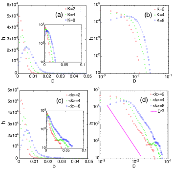
Figure 2: (Color online) The number of times $h$ when a particular value of the fitness difference $D$ between a local optimum and $n_{omv}$ occurs in the rugged fitness landscapes. Here the ’quenched’ models have been adopted. (c) and (d) [(a) and (b)] show the histograms and the tails for the scale-free [random] networks of $\langle k\rangle=(K=)2$ ($\bigcirc$), $4$ ($\Box$), $8$ ($\triangle$), respectively, where $N=256$. Here $\langle k\rangle$ stands for the average degree of nodes. The data for 1000 samples are superimposed in each figure. (b) and (d) (inset) are shown in the log-log (semi-log) plot of the tails.

IV Numerical results

IV.1 Rugged fitness landscapes

Fig.1 shows the rugged fitness landscapes of both the ’quenched’ random $NK$ and the ’quenched’ $SF$ Kauffman models. Here we have calculated the systems up to $N=256$. This is just because of our computer power at this moment. We only show the data for $N=256$ in this paper. As previously noted by KauffmanKauffmanBook1 the fitness landscapes of the random networks are very rugged. We see that the fitness landscapes of scale-free networks are very rugged as well, but quite different from those of the random networks. This can be understood as follows: In the random network each one of the nodes always meets with the same $K$ links to the neighbors. The ruggedness can be dominantly bounded by the value of $K$. Hence, as $K$ becomes large, the fluctuations in the rugged fitness landscapes become large. On the other hand, in the scale-free network there are various kinds of degrees $k_{i}$ of nodes. In other words, each node has its own $k_{i}$ links and there is the distribution of the degrees such as $P(k)\propto k^{-\gamma}$. The AB model exhibits power-law with $\gamma=3$. Therefore, the fitness landscapes can fluctuate, according to the degree distribution of the network. So, as the degree $k_{i}$ of a node is large, the difference in the fitness between the optimum and the mutants is expected to be large. Hence, the fitness landscapes obey the nature of the scale-free network.

IV.2 Histograms and tails of rugged fitness landscapes

How can we detect the differences in the rugged fitness landscapes between the random and the scale-free networks? To do so, denote by $h$ the histogram and denote by $D$ the fitness difference between the local optimum and the one-mutant variant. Then we draw the histograms of the rugged fitness landscapes in the normal plot [(a) and (c)], in the log-log plot [(b) and (d)], and in the semi-log plot (insets), respectively (Fig.2). Comparing (a) with (c) in the numerical results, we find that the histograms of the fitness landscapes for the random networks behave like Gaussian distributions, which can be fitted by $h\propto e^{-(D-\langle D\rangle)^{2}/v^{2}}$ where we set the peak value as $\langle D\rangle$, the variance as $v=\sqrt{\langle(\Delta D)^{2}\rangle}$ with $\Delta D=D-\langle D\rangle$. We have found numerically that $\langle D\rangle=\{0.943,2.62,5.85\}\times 10^{-3}$; $v=\{4.31,5.75,7.58\}\times 10^{-3}$ for $K=2,4,8$, respectively. On the other hand, the histograms for the scale-free networks behave like non-Gaussian distributions with a broad tail, which can be fitted by

$$h\propto\left\{\begin{array}[]{ll}e^{-\frac{(D-\langle D\rangle)^{2}}{v^{2}}}&\mbox{if $(D-\langle D\rangle)^{2}\ll v^{2}$}\\ e^{-\alpha\frac{D-\langle D\rangle}{v}}&\mbox{if $D$ is comparable to $\langle D\rangle$}\\ D^{-\beta}&\mbox{if $D$ is much larger than $\langle D\rangle$}\end{array}\right..$$

Here we have found numerically that $\langle D\rangle=\{1.48,2.74,5.27\}\times 10^{-3}$; $v=\{3.45,4.67,5.53\}\times 10^{-3}$; $\alpha=1.30,1.21,0.978$; $\beta=3.11,3.50,2.98$, for $\langle k\rangle=2,4,8$, respectively.

We note here the following: (a) The tail (i.e., scaling behavior) appears when the system size becomes as large as $N=256$. And as the value of $\langle k\rangle$ is increasing, the value of $\beta$ seems closer to $\gamma=3$ of $P(k)$ in the AB modelBarabasi [Fig.2 (d)]. But in view of the limited accuracy of Fig. 2(d) (e.g., $\beta=3.50,2.98$), at the present moment this can be a conjecture, speculated from the numerical results for the system of $N=256$. However, in Appendix A we give a sharp analytical arguments showing a strict relationship between the power-law decay and the ”degree” fluctuations. And also, since we extend the system up to $N=1024$, we are able to confirm ourselves that the tail behavior is maintained and become more prominent, as $N$ is increasing. As an example, we show the result in Appendix B.

(b) The results for the random networks show a kind of transition when the value of $K$ is going up from $K=2$ to $K=8$. This is consistent with the critical value of $K_{c}=2$ for $p=0.5$ which was analytically obtained from the annealed modelDerridaPomeau . Therefore, the distribution below $K_{c}$ is quite different from that above $K_{c}$ so that the distributions for $K>K_{c}$ become more Gaussian-like as $K$ increases. Very interestingly, we find a similar transition for the scale-free networks as well, when the value of $\langle k\rangle$ is going up from $\langle k\rangle=2$ to $\langle k\rangle=8$.

This can be explained as follows: Suppose the distribution of degrees is approximately given by $P(k)=k^{-\gamma}/\zeta(\gamma)$ such that we can impose normalization $\sum_{k=1}^{\infty}P(k)=1$, where $\zeta(\gamma)$ is the Riemann’s zeta function defined by $\zeta(\gamma)=\sum_{k=1}^{\infty}k^{-\gamma}$. Substituting it to the definition $\langle k\rangle=\sum_{k=1}^{\infty}kP(k)$, then we obtain

$$\langle k\rangle=\zeta(\gamma-1)/\zeta(\gamma),$$

which is finite for $\gamma>2$ and infinite for $1<\gamma<2$ and which was first obtained by Aldana et. al.Aldana . For example, since $\gamma=3$ for the special case of the AB model, we obtain $\langle k\rangle=\zeta(2)/\zeta(3)=1.64493\cdots/1.20205\cdots\approx 1.3684$. As studied by Aldana et. al.AldanaCK ; Aldana , the critical value $\langle k\rangle_{c}$ for the annealed dynamics of the $SF$ Kauffman model is given by $\langle k\rangle_{c}=\zeta(\gamma_{c}-1)/\zeta(\gamma_{c})=2$ for $p=0.5$ as well, where $\gamma_{c}\approx 2.47875$. Within the limited accuracy of our numerical results (some 20 percent) this is the same value as just stated for the quenched dynamics. In fact, we expect that also for our quenched dynamics there is a critical point around $\langle k\rangle_{c}=2$ , with $\beta$ around 3, maybe again exactly at these values. In fact, in appendix A we show that also in our case the statistics of the rugged fitness landscape is bounded by $K$, such that $\beta$ reflects the fluctuations of the ’degree’, which should be the same both for the quenched and the annealed dynamics AldanaCK ; Aldana . Thus, our numerical results support this analytical result although our system is not very large but a finite scale-free network of $N=256$. We also note here that we confirm that the phase transition at the critical value of $\langle k\rangle=\langle k\rangle_{c}=2$, which was proved analytically in the ’annealed’ model by Aldana et.al. Aldana , occurs in the ’quenched’ model as well IKY .

IV.3 The correlation between the fitness of local optima and their Hamming distance from the highest optimum found

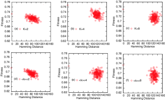
Figure 3: (Color online) The correlation between the fitness of local optima and their Hamming distance from the highest optimum found. It is shown for the random networks with $K=2$ (a), $4$ (b), $8$ (c) and for the scale-free networks with $\langle k\rangle=2$ (d), $4$ (e), $8$ (f), respectively, where $N=256$. The vertical axis stands for the fitness and the horizontal axis the Hamming distances between the largest local optimum and the local optima. The data for 1000 samples are superimposed in each figure. In both cases there seem to exist phase transitions, i.e., at $K=K_{c}=2$ for the random networks and $\langle k\rangle=\langle k\rangle_{c}=2$ for the scale-free networks, supporting the exact statement for the ’annealed’ version of the first mentioned case and the analytical prediction of Aldana et. al. on the annealed version of the $SF$ model.

Finally we present the correlation between the fitness of local optima and their Hamming distance from the highest optimum foundKauffmanBook1 (Fig.3). In both the random and the scale-free networks we find the following: If $K$ and $\langle k\rangle$ are as small as the critical value of $2$, then the highest optima are nearest to one another. And the optima at successively greater Hamming distances from the highest optimum are successively less fit. Therefore, there is a global order to the landscape. On the other hand, as $K$ and $\langle k\rangle$ increase, the correlations fall away. This shows that the previous assertions are maintained in the correlations, respectively.

V Conclusions

In conclusion, we have studied the structure and statistics of the rugged fitness landscapes for the quenched $SF$ Kauffman models, comparing with that for the quenched random $NK$ Kauffman models. We have numerically calculated the rugged fitness landscapes, the distributions, the tails, and the fitness correlations of local optima with the Hamming distance from the highest optimum, respectively. From the results, we have concluded that in the $SF$ Kauffman models there is a transition of network when $\langle k\rangle=\langle k\rangle_{c}=2$, while in the $NK$ Kauffman models such a transition occurs at $K=K_{c}=2$. This is, in some sense, quite analogous to the situation in the study of Boolean dynamics of $NK$ and $SF$ Kauffman modelsAldanaCK . It would be very interesting if we could apply this approach to study fitness landscapes of other network systems.

Appendix A Analytical arguments of relation between the power-law decay and the ’degree’ fluctuations

The tail behavior of the histogram is interpreted as follows.

Define a network with $N$ nodes, which can be any kind of network such as random, scale-free and exponential-fluctuating networks, where the $i$-th node has $k_{i}$ degree (i.e., link number). Let us consider the Kauffman model. As given in Table 1, the number of inputs to the $i$-th node is given by $k_{i}+1$. Let us now choose an $N$-dimensional initial state $A$ such as $(1,0,0,1,1,\cdots,1)$. Considering the input from the given network structure, we can define fitness $W_{i}$ on each node. Therefore, we can define the fitness $W_{A}$ of the state $A$ by

$$W_{A}=\frac{1}{N}\sum_{j=1}^{N}W_{j}^{A},$$

where $W_{j}^{A}$ means fitness at the $j$-th node in the state $A$. Consider one-mutant family of the initial state $A$, in which there are $N$ neighbor states with Hamming distance one. For example, let us say one of them, $B$ and define as $(0,0,0,1,1,\cdots,1)$. In this example, only the state of node 1 is different from 1 to 0. Therefore, the difference in input values between the initial state $A$ and this state $B$ comes from nodes linked to node 1. This situation provides a difference in fitness.

Suppose that the degree of node 1 is $k_{1}$ and denote the $k_{1}$ nodes linked to node 1 by $j_{1},\cdots,j_{k_{1}}$. The values of nodes linked to node 1 are given different random numbers $W_{i}^{\prime}$ according to Table 1. We then obtain fitness for the state $B$ as

$$W_{B}=\frac{1}{N}\sum_{j=1}^{N}W_{j}^{B}=\frac{1}{N}(W_{1}^{\prime}+W_{j_{1}}^{\prime}+\cdots+W_{j_{k_{1}}}^{\prime}+\cdots).$$

Thus, a genetic mutation in the state of one-mutant gives a change only for the node that the mutation occurred and the nodes linked to it. Therefore, if we consider only the fitness difference from the local optimum, then the fitness value of the one-mutant family that has Hamming distance 1 from the local optimum state depends upon which node the mutation occurs. Hence, in the case that there is mutation on node $m$, we obtain

$$\Delta W_{B}(m)=\frac{1}{N}(\Delta W_{1}+\Delta W_{j_{1}}+\cdots+\Delta W_{j_{k_{1}}}),$$

where $\Delta W_{j}=W_{j}^{\prime}-W_{j}$. The left hand side of Eq.(A3) means the fitness difference, $D$. To see what it means, let us define the averaged fitness difference for node $m$:

$$\langle D_{B}(m)\rangle=\frac{1}{k_{m}+1}(\Delta W_{1}+\Delta W_{j_{1}}+\cdots+\Delta W_{j_{k_{m}}}).$$

We then have

$$D_{m}=\Delta W_{B}(m)=\frac{1}{N}\langle D_{B}(m)\rangle(k_{m}+1).$$

From this, if the average $\langle D_{B}(m)\rangle$ is constant, then $D_{m}$ is proportional to $k_{m}+1$. But, more generally, there are two contributions: one from random number $W_{i}$ in $\Delta W_{1}+\Delta W_{j_{1}}+\cdots+\Delta W_{j_{k_{m}}}$ and another from degree $k_{m}$. Here, if the random numbers are defined by a uniform distribution, then we can understand that they contribute to the exponent of the fitness distribution function and the tail of the distribution function comes from that of the degree (link number). Because, since the maximum value of $W_{i}$ is 1, it is bounded as

$$|\Delta W_{1}+\Delta W_{j_{1}}+\cdots+\Delta W_{j_{k_{m}}}|\leq k_{m}+1.$$

Hence, this provides

$$|D_{m}|\leq\frac{k_{m}+1}{N}.$$

From the above, in the $NK$ model the statistics of rugged fitness landscapes is bounded by $K$. In the $SF$ model, since $k_{i}$ is distributed by a power law, the statistics becomes the same power distribution. Similarly, in the exponential fluctuation distribution, so is the fitness distribution. In this way, the statistics of fitness is strongly dominated by that of the link distribution in the network.

Appendix B Tail behavior of the system of $N=1024$

We show the tail behavior of the histogram in the system size of $N=1024$ in Fig.4. This may support our assertion in the text. We find again $\gamma\approx 3$ ; but since here the power-law decay is already obtained for $<k>=2$, we cannot exclude that$<k>_{c}<2$, although such a statement would perhaps only reflect finite-size effects.

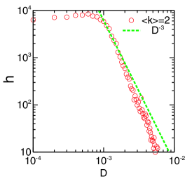
Figure 4: (Color online) $log$-$log$ plot of the tail behavior of the histogram for scale-free networks of the system size $N=1024$, where $\langle k\rangle=2$. Here the ’quenched’ models have been adopted. The vertical axis means $\log$ of the number of times $h$ when a particular value of the fitness difference $D$ between a local optimum and $n_{omv}$ occurs in the rugged fitness landscapes. The horizontal axis means $log$ of the fitness difference $D$. The data for 100 samples are superimposed in figure. We confirm ourselves that $\gamma\approx 3$.

References

- (1) e-mail: kazumoto@stannet.ne.jp.
- (2) e-mail: f01j006g@mail.cc.niigata-u.ac.jp.
- (3) e-mail: hyamada@uranus.dti.ne.jp.
- (4) J. Maddox, What Remains To Be Discovered, (Touchstone, NY, 1998).
- (5) M. Eigen, Naturewissenschaften 58, 465-523 (1971).
- (6) S. A. Kauffman, The Origins of Order (Oxford University Press, New York, 1993) and references therein.
- (7) P. Erdös and A. Rényi, Publ. Math. 6, 290-297 (1959); Publ. Math. Inst. Hung. Acad. Sci. 5, 17-61 (1960); Acta Math. Acad. Sci. Hung. 12 261-267 (1961).
- (8) B. Derrida and Y. Pomeau, EuroPhys. Lett. 1, 45-49 (1986). B. Derrida and G. W. Weisbuch, J. Physique 47, 1297-1303 (1986).
- (9) U. Bastolla and G. Parisi, Physica D 98, 1-25 (1996).
- (10) M. E. J. Newman, SIAM Review 45, 167-256 (2003) and references therein.
- (11) M. Aldana, S. Coppersmith and L. P. Kadanoff, nonlin AO/0204062 (2002) and references therein.
- (12) J. J. Hopfield, Proc. Natl. Acad. Sci. USA 79, 2554-2558 (1982).
- (13) P. W. Anderson, in Emerging Syntheses in Science, Proc. Founding Workshops of the Santa Fe Institute, ed. D. Pines, (Santa Fe Institute, Santa Fe, 1987), pp.17-20.
- (14) S. H. Strogatz, Nature 410, 268-276.
- (15) A.-L. Barabási, Linked, (Penguin books, London, 2002) R. Albert and A.-L. Barabási, Rev. Mod. Phys. 74, 47-97 (2002) and references therein.
- (16) S. N. Dorogovtsev and J. F. F. Mendes, Evolution of Networks, (Oxford University Press Inc., New York, 2003) and references therein.
- (17) B. Luque and R. V. Solé, Phys. Rev. E 55, 257-260 (1997).
- (18) R. Albert and A.-L. Barabási, Phys. Rev. Lett. 84, 5660-5663 (2000).
- (19) J. J. Fox and C. C. Hill, Chaos 11, 809-815 (2001).
- (20) C. Oosawa and A. Savageau, Physica D 170, 143-161 (2002).
- (21) X. F. Wang and G.-R. Chen, IEEE Trans. Cir. Sys. 49, 54-61 (2002).
- (22) M. Aldana, Physica D 185, 45-66 (2003). M. Aldana and P. Cluzel, Proc. Natl. Acad. Sci. USA 100, 8710-8714 (2003).
- (23) R. Serra, M. Villani, and L. Agostini, ”A Small-World Network Where All Nodes Have The Same Connectivity, With Application To The Dynamics Of Boolean Interacting Automata”, in On the Dynamics of Scale-Free Boolean Networks, Lecture Notes on Computer Science 2859, (Springer-Verlag, Berlin Heidelberg, 2003), pp. 43-49.
- (24) A. Castro e Silva, J. Kamphorst Leal da Silva, and J. F. F. Mendes , Phys. Rev. E 70, 066140 (2004).
- (25) As similar as in the Boolean dynamical models KauffmanBook1 ; DerridaPomeau ; BasParisi ; Newman ; AldanaCK , if we fix the set of the randomly chosen real output in the course of steps for the average, then we call the model the quenched model. On the other hand, if we change the set at each step, then we call it the annealed model. In this paper, we only study the quenched model for the later purposes.
- (26) K. Iguchi, S. Kinoshita, and H. Yamada, Boolean Dynamics of Kauffman Models with A Scale-free Network, in preparation, (2005).