Continuous quantum feedback of coherent oscillations in a solid-state qubit

Abstract

We have analyzed theoretically the operation of the Bayesian quantum feedback of a solid-state qubit, designed to maintain perfect coherent oscillations in the qubit for arbitrarily long time. In particular, we have studied the feedback efficiency in presence of dephasing environment and detector nonideality. Also, we have analyzed the effect of qubit parameter deviations and studied the quantum feedback control of an energy-asymmetric qubit.

I Introduction

Continuous quantum feedback in optics and atomic physics has been studied theoretically Wiseman ; Tombesi ; Hofmann ; Wang ; Doherty for more than a decade (see also Refs. Shapiro, ; Yamamoto, ; Caves-87, ; Wiseman-94, ; Doherty-3, ) and has been recently demonstrated experimentally.Geremia In contrast, continuous quantum feedback in solid-state mesoscopics is a relatively new subject. Ruskov-02 ; Ruskov-SPIE ; Korotkov-04 ; Hopkins ; Ruskov-squeez The use of quantum feedback to maintain coherent (Rabi) oscillations in a qubit for arbitrarily long time has been proposed and analyzed in Refs. Ruskov-02, and Ruskov-SPIE, ; a simplified experiment has been proposed in Ref. Korotkov-04, . Cooling of a nanoresonator by quantum feedback has been proposed and analyzed in Ref. Hopkins, . The use of quantum feedback for the nanoresonator squeezing has been studied in Ref. Ruskov-squeez, .

Feedback control of a quantum system requires continuous monitoring of its evolution (in ideal case the wavefunction should be monitored), which is the main non-trivial feature of quantum feedback. Obviously, the operation of quantum feedback cannot be analyzed using the “orthodox” approach of instantaneous collapse, Neumann which is not suitable for continuous quantum measurement. Also, the ensemble-averaged (“conventional”) approach Caldeira to continuous quantum measurement is not suitable since it cannot describe random evolution of a single quantum system. Therefore, analysis of quantum feedback requires a special theory capable of describing continuous measurement of a single quantum system.

The development of such theories has started long ago Mensky ; Gisin ; Caves-86 and has attracted most of attention in quantum optics Wiseman ; Carmichael ; Plenio (in spite of similar underlying principles, the theories may differ significantly in formalism and area of application). For solid-state qubits such theory (“Bayesian” formalism) has been developed relatively recently Kor-99 ; Kor-01 (for review see Ref. Kor-rev, ). The equivalence of the Bayesian formalism to the quantum trajectory approach translated Goan ; Goan-2 ; Oxtoby from quantum optics has been shown in Ref. Goan, .

In simple words, the Bayesian formalism takes into account the information contained in the noisy output of the solid-state detector measuring the qubit, so that the corresponding quantum back-action onto qubit evolution is described explicitly. In classical probability theory the way to deal with an incomplete information is via the Bayes formula;Feller it can be shown Kor-99 ; Kor-01 ; Kor-rev that a somewhat similar procedure should be used for evolution of the qubit density matrix due to continuous measurement, that explains why the formalism is called Bayesian. The Bayesian formalism shows that an ideal (quantum-limited) detector can monitor precisely the random evolution of the qubit wavefunction in the course of measurement; and if the measurement starts with a mixed state, the qubit density matrix is gradually purified, eventually approaching a pure state. The quantum point contact (QPC) is an example of (theoretically) ideal detector. When the detector does not have 100% quantum efficiency [as in the case of a single-electron transistor (SET)], there is an extra dephasing term in the evolution equation, so that the qubit purification due to gradually acquired information competes with the decoherence due to detector nonideality.

The possibility to monitor the random quantum evolution of the qubit in the process of measurement naturally allows us to arrange a feedback loop which keeps the qubit evolution close to a desired “trajectory”. Of course, the measurement process disturbs the qubit evolution; however, the detector output contains enough information to monitor and undo the effect of this disturbance. It is important that the deviations from the desired trajectory due to interaction with decohering environment are efficiently suppressed by the feedback loop, that can be useful, for example, in a quantum computer. The feedback loop considered in Refs. Kor-01, and Ruskov-02, has been designed to maintain the coherent oscillations in the qubit for arbitrarily long time by comparing the oscillation phase with the desired value and keeping the phase difference close to zero (the amplitude of oscillations is equal to unity in the case of ideal detector and energy-symmetric qubit). It has been shown that the fidelity of such feedback loop can be arbitrarily close to 100%, while it decreases in the case of a nonideal detector and/or significant interaction with environment as well as in the case of finite bandwidth of the line carrying the signal from detector.

The present paper is a more detailed analysis of the operation of the feedback loop proposed in Refs. Kor-01, and Ruskov-02, . In particular, we study the feedback loop operation in presence of extra dephasing due to environment and nonideal detector, analyze the effect of qubit parameter deviation, and consider the feedback of a qubit with energy asymmetry. In the next Section we describe the model, in Section III we consider the feedback operation in the ideal case, Section IV is devoted to the effects of nonideal detector and extra dephasing, in Section V we analyze the worsening of feedback efficiency in the case of qubit parameter deviations, in Section VI we study the feedback of an energy-asymmetric qubit, and Section VII is a conclusion.

II Model

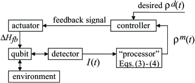
Figure 1: Schematic of the quantum feedback loop maintaining the quantum oscillations in a qubit. The qubit oscillations affect the current $I(t)$ through a weakly coupled detector; this signal is translated by the “processor” into continuously monitored value $\rho^{m}(t)$ of the qubit density matrix. Next, by comparing $\rho^{m}(t)$ with the desired oscillating state $\rho^{d}(t)$, a certain algorithm (“controller”) produces the feedback signal applied to an “actuator” which changes the qubit tunneling amplitude $H+\Delta H_{fb}$, in order to reduce the difference between $\rho^{m}$ and $\rho^{d}$.

Let us consider the quantum feedback loop shown in Fig. 1, which controls the qubit characterized by the Hamiltonian

$${\cal H}_{qb}=\frac{\varepsilon_{fb}}{2}\,(c_{2}^{\dagger}c_{2}-c_{1}^{\dagger}c_{1})+H_{fb}(c_{1}^{\dagger}c_{2}+c_{2}^{\dagger}c_{1}),$$ (1)

where $c_{1,2}^{\dagger}$ and $c_{1,2}$ are creation and annihilation operators corresponding to two “localized” states of the qubit, representing the “measurement basis”. The qubit energy asymmetry $\varepsilon_{fb}$ and tunneling amplitude $H_{fb}$ can both be controlled by the feedback loop:

$$H_{fb}=H+\Delta H_{fb},\hskip 14.22636pt\varepsilon_{fb}=\varepsilon+\Delta\varepsilon_{fb};$$ (2)

however, in this paper we assume $\Delta\varepsilon_{fb}=0$, so that only tunneling is controlled. Intrinsic frequency of coherent oscillations in the qubit (without interaction and feedback) is $\Omega=\sqrt{4H^{2}+\varepsilon^{2}}/\hbar$; we also call it Rabi frequency, not implying presence of microwave radiation (despite this terminology differs from the initial meaning of Rabi oscillations, it is conventionally used nowadays).

For definiteness we consider a “charge” qubit continuously measured by QPC or SET, so that the measurement setup is similar to what has been studied theoretically, e.g. in Refs. Gurvitz, ; Shnirman-98, ; Kor-99, ; Kor-01, ; Kor-rev, ; Averin, ; Goan, ; Goan-2, ; Oxtoby, ; Buttiker, ; Clerk, . Taking into account the quantum back-action due to measurement, the evolution of the qubit density matrix $\rho$ is described by the Bayesian equations Kor-99 ; Kor-01 ; Kor-rev (in Stratonovich form)

$$\dot{\rho}_{11}=-2\,\frac{H_{fb}}{\hbar}\,\mbox{Im}\rho_{12}+\rho_{11}\rho_{22}\,\frac{2\Delta I}{S_{I}}\,[I(t)-I_{0}],$$ (3)

$${\dot{\rho}}_{12}=i\,\frac{\varepsilon_{fb}}{\hbar}\,\rho_{12}+i\,\frac{H_{fb}}{\hbar}\,(\rho_{11}-\rho_{22})$$

$$-(\rho_{11}-\rho_{22})\frac{\Delta I}{S_{I}}\,[I(t)-I_{0}]\,\rho_{12}-\gamma\rho_{12}\,,$$ (4)

where $I(t)$ is the noisy detector current (output signal), $S_{I}$ is the spectral density of current noise, $\Delta I=I_{1}-I_{2}$ is the difference between two average currents $I_{1}$ and $I_{2}$ corresponding to the two qubit states, and $I_{0}=(I_{1}+I_{2})/2$. The dephasing rate $\gamma=\gamma_{d}+\gamma_{env}$ has the contribution $\gamma_{d}$ due to detector nonideality, $\gamma_{d}=(\eta^{-1}-1)(\Delta I)^{2}/4S_{I}$ (here $\eta\leq 1$ is the quantum efficiency Kor-99 ; Kor-01 ; Kor-rev ; Averin ; Buttiker ; Clerk ) and contribution $\gamma_{env}$ due to interaction with extra environment. As always, $\rho_{11}+\rho_{22}=1$ and $\rho_{21}=\rho_{12}^{*}$. Equations (3)–(4) imply weak detector response $|\Delta I|\ll I_{0}$, quasicontinuous current, and large detector voltage compared to the qubit energy. The current

$$I(t)=I_{0}+(\Delta I/2)(\rho_{11}-\rho_{22})+\xi(t)$$ (5)

has the pure noise contribution $\xi(t)$ with frequency-independent spectral density $S_{I}$. Notice that averaging of Eqs. (3)–(4) over $\xi(t)$ leads to the standard ensemble-averaged equations Caldeira with ensemble dephasing rate $\Gamma=(\Delta I)^{2}/4S_{I}+\gamma$. We characterize coupling between qubit and detector by the dimensionless constant ${\cal C}=\hbar(\Delta I)^{2}/S_{I}H$ (we assumeH-sign $H>0$) and concentrate on the case of weak coupling ${\cal C}\lesssim 1$ (notice that ${\cal C}=1$ can still be considered a weak coupling since the quality factor of oscillations in presence of measurement Kor-sp is $8\eta/{\cal C}$ for $\varepsilon=0$).

In this paper we consider the “Bayesian” feedback, Ruskov-02 which requires a “processor” solving Eqs. (3)–(4) in real time – see Fig. 1 (other possibilities are, for example, “direct” feedback briefly mentioned in Ref. Ruskov-02, and “simple” feedback via quadrature components analyzed in Ref. Korotkov-04, ). In this paper we neglect the effect of finite bandwidth Ruskov-02 ; Ruskov-SPIE ; Oxtoby-2 of the line carrying the detector signal, and we also neglect the signal delay in the feedback loop. As a result, in most of the paper we assume that the monitored value $\rho^{m}(t)$ of the qubit density matrix coincides with the actual value $\rho(t)$. Only in Section V we consider $\rho^{m}$ different from $\rho$ because of the deviation of the qubit parameters $H$ and $\varepsilon$ from the values assumed in the “processor” (finite signal bandwidth would also lead to difference between $\rho$ and $\rho^{m}$).

For the feedback control the monitored qubit evolution is compared with the desired evolution (Fig. 1), and the difference signal is used to control the qubit parameters in order to decrease the difference. Actually, various algorithms (“controllers”) are possible for this purpose; in this paper we will consider linear control (see below). We study the feedback loop, which goal is to maintain perfect coherent oscillations in the qubit for arbitrarily long time, and (except for Section VI) the desired evolution is

$$\rho_{11}^{d}=\frac{1+\cos\Omega_{0}t}{2},\hskip 8.5359pt\rho_{12}^{d}=i\,\frac{\sin\Omega_{0}t}{2},$$ (6)

with frequency $\Omega_{0}=2H/\hbar$ corresponding to $\varepsilon=0$. Except for Section VI, we assume the following feedback control:

$$\Delta H_{fb}=-FH\Delta\phi_{m},$$ (7)

$$\Delta\phi_{m}=\phi_{m}(t)-\Omega_{0}t\,\,\,(\mbox{mod}\,2\pi),$$ (8)

$$\phi_{m}(t)=\mbox{arctan}[2\,\mbox{Im}\rho_{12}^{m}/(\rho_{11}^{m}-\rho_{22}^{m})]\,\,$$

$$\hskip 14.22636pt+(\pi/2)[1-\mbox{sgn}(\rho_{11}^{m}-\rho_{22}^{m})],$$ (9)

where $\phi_{m}$ is the monitored value of the phase, phase difference $\Delta\phi_{m}$ is defined as $|\Delta\phi_{m}|\leq\pi$, and $F$ is a dimensionless feedback factor [the second term in Eq. (9) provides proper phase continuity on $2\pi$ circle]. The controller (7) is supposed to decrease the phase difference (negative feedback): if phase $\phi_{m}(t)$ is ahead of the desired value, then $\Delta H_{fb}$ is negative, that slows down the qubit oscillations and decreases the phase shift; if $\phi_{m}(t)$ is behind the desired value, the oscillation frequency increases to catch up.

We will characterize the feedback efficiency by the “synchronization degree” $D$ defined as averaged over time scalar product of two Bloch vectors corresponding to the desired and actual states of the qubit. An equivalent definition is

$$D=2\langle\mbox{Tr}\rho\rho^{d}\rangle-1,$$ (10)

where $\langle..\rangle$ denotes averaging over time. Perfect feedback operation corresponds to $D=1$ (notice that $\rho^{d}$ is a pure state). Feedback efficiency $D$ can be easily translated into average fidelity as $(D+1)/2$ or $\sqrt{(D+1)/2}$, depending on the definition of fidelity Jozsa ; Doherty-3 (translation formula would be slightly longer if neither $\rho$ nor $\rho^{d}$ are pure states). We prefer to use $D$ instead of fidelity because $D=0$ in absence of feedback when $\rho$ and $\rho^{d}$ are completely uncorrelated, while fidelity is non-zero.

III Ideal case

Let us start analysis with the basic ideal case of $\eta=1$ (quantum-limited detector, e.g. QPC), absence of extra environment ($\gamma_{env}=0$), and symmetric qubit ($\varepsilon=0$). The analytical results for this case have been presented in Ref. Ruskov-02, ; here we discuss the derivation in more detail.

Since $\eta=1$ and $\gamma_{env}=0$, so that there is no dephasing term in Eq. (4), the qubit density matrix $\rho$ becomes pure in the process of measurement. Kor-rev Because of the energy symmetry, $\varepsilon_{fb}=\varepsilon=0$, the real part of $\rho_{12}$ eventually becomes zero. This happens because the product $(\rho_{11}-\rho_{22})(I-I_{0})$ affecting the evolution of $\mbox{Re}\rho_{12}$ in Eq. (4) is on average positive. Therefore, after a transient period the evolution of the density matrix $\rho$ can be parameterized as

$$\rho_{11}=(1+\cos\phi)/2,\,\,\,\,\rho_{12}=i(\sin\phi)/2$$ (11)

with only one parameter $\phi(t)$. We have also checked this fact numerically. Notice that since the qubit is monitored exactly, $\rho=\rho^{m}$, the phase $\phi$ coincides (modulo $2\pi$) with the monitored phase $\phi_{m}$ defined by Eq. (9).

The evolution equation for phase $\phi$ can be easily derived from Eq. (4) as

$$\dot{\phi}=2H_{fb}/\hbar-(\Delta I/S_{I})(I-I_{0})\sin\phi,$$ (12)

so the phase difference $\Delta\phi=\phi-\Omega_{0}t$ (which coincides with $\Delta\phi_{m}$) evolves as

$$\frac{d}{dt}\,\Delta\phi=-\sin\phi\,\frac{\Delta I}{S_{I}}\left(\frac{\Delta I}{2}\,\cos\phi+\xi\right)-F\Omega_{0}\,\Delta\phi.$$ (13)

(All equations are in the Stratonovich form, so we use usual rules for derivatives.Oksendal ) Notice that because of our definition $|\Delta\phi|\leq\pi$, the phase difference jumps by $\pm 2\pi$ at the borders of $\pm\pi$ interval.

For weak coupling (${\cal C}/8\ll 1$) the qubit oscillations are only slightly perturbed by measurement and corresponding phase diffusion is relatively slow. Assuming that the feedback control is also slow on the timescale of oscillations ($|\Delta H_{fb}|\ll H$), we can average Eq. (13) over relatively fast oscillations. Then the first term in parentheses is averaged to zero and averaging of the term $-(\sin\phi)(\Delta I/S_{I})\xi(t)$ leads to the effective noise $\tilde{\xi}(t)$ with spectral density $S_{\tilde{\xi}}=(\Delta I)^{2}/2S_{I}$, so that the remaining slow evolution of phase difference is

$$\frac{d}{dt}\,\Delta\phi=\tilde{\xi}-F\Omega_{0}\,\Delta\phi.$$ (14)

To find the feedback efficiency $D=\langle\cos\Delta\phi\rangle$ analytically, let us also assume that feedback performance is good enough to keep the phase difference $\Delta\phi$ well inside the $\pm\pi$ interval, so that the phase slips (jumps of $\Delta\phi$ by $\pm 2\pi$) occur sufficiently rare. In this case we can consider Eq. (14) on the infinite interval of $\Delta\phi$. The corresponding Fokker-Planck-Kolmogorov equation for the probability density $\sigma(\Delta\phi)$

$$\frac{\partial\sigma}{\partial t}=\frac{\partial}{\partial\Delta\phi}\left(\sigma\,F\Omega_{0}\,\Delta\phi\right)+\frac{1}{4}\,\frac{\partial^{2}(S_{\tilde{\xi}}\sigma)}{\partial(\Delta\phi)^{2}}$$ (15)

has the Gaussian stationary solution $\sigma_{st}(\Delta\phi)=(2\pi{\cal V})^{-1/2}\linebreak[1]\exp[-(\Delta\phi)^{2}/2{\cal V}]$ with variance ${\cal V}=S_{\tilde{\xi}}/4F\Omega_{0}={\cal C}/16F$. Therefore, $\langle\cos\Delta\phi\rangle=\linebreak[1]\exp(-{\cal V}/2)$, and so the feedback efficiency is Ruskov-02

$$D=\exp(-{\cal C}/32F)$$ (16)

in the case of weak coupling and sufficiently efficient feedback (${\cal C}\lesssim 1$, $D\gtrsim 1/2$).

Figure 2: Solid lines: quantum feedback efficiency $D$ as a function of the feedback strength $F$ for five different values of the coupling ${\cal C}$ and ideal operation conditions (see text). The curves for ${\cal C}\leq 3$ practically coincide with each other. Dashed line shows the analytical result (16). Inset shows the same curves for larger range of $F/{\cal C}$.

Figure 2 shows comparison between the analytical result (16) and numerical results for $D$ as a function of feedback factor $F$ (scaled by coupling ${\cal C}$). Numerical results have been obtained by direct simulation of the Bayesian equations (3)–(4) using the Monte Carlo method Kor-99 ; Kor-01 for five values of coupling: ${\cal C}=10$, 3, 1, 0.3, and 0.1. One can see that for weak coupling ${\cal C}\lesssim 1$ the analytics works very well when the feedback is sufficiently efficient, $D\gtrsim 0.5$. Another important observation is that with the feedback factor $F$ normalized by coupling ${\cal C}$, the curves for ${\cal C}\leq 1$ are practically indistinguishable from each other, the curve for ${\cal C}=3$ goes a little higher but still within the line thickness, and only the curve for ${\cal C}=10$ is noticeably different. Therefore, as expected, the weak-coupling limit is practically reached starting with ${\cal C}\leq 1$. This makes unnecessary to analyze numerically the case of very small coupling ${\cal C}\ll 1$, which requires much longer simulation time than the case of moderately small coupling.

Notice that $|\Delta H_{fb}|/H<\pi F$, and $F$ scales with coupling ${\cal C}$. Therefore, in the experimentally realistic case ${\cal C}\ll 1$ a typical amount of the parameter change due to feedback is small, $|\Delta H_{fb}|\ll H$. [Hence, we should not worry about unnatural assumption of using control equation (7) even when $H_{fb}$ becomes negative.]

The feedback efficiency $D$ is directly related Korotkov-04 to the average in-phase quadrature component of the detector current, $\langle I(t)\cos\Omega_{0}t\rangle=(\Delta I/4)[D+\langle\cos(2\Omega_{0}t+\Delta\phi)\rangle]$, so that in the case of practically harmonic oscillations $D=(4/\Delta I)\langle I(t)\cos\Omega_{0}t\rangle$. Positive in-phase quadrature is one of easy ways to verify the quantum feedback operation experimentally.

Besides analyzing feedback efficiency $D$, let us also calculate the qubit correlation function $K_{z}(\tau)=\langle z(t+\tau)\,z(t)\rangle$ where $z=\rho_{11}-\rho_{22}$. In the case of practically harmonic (weakly disturbed) oscillations, the correlation function $K_{z}(\tau)=\langle\cos[\phi(t+\tau)]\cos[\phi(t)]\rangle$ is equal to $\langle\cos[\Omega_{0}\tau+\delta\phi(\tau)]\rangle/2$ where $\delta\phi(\tau)=\Delta\phi(t+\tau)-\Delta\phi(t)$ is the phase deviation during time $\tau$. Since in our case $\langle\sin\delta\phi(\tau)\rangle=0$ because of the symmetry of Eq. (14), the correlation function is reduced to

$$K_{z}(\tau)=\frac{\cos\Omega_{0}\tau}{2}\,\langle\cos\delta\phi(\tau)\rangle.$$ (17)

We can find $\langle\cos\delta\phi(\tau)\rangle$ using exact solution of the Fokker-Planck-Kolmogorov equation (15) with initial condition $\sigma(\Delta\phi,0)=\delta(\Delta\phi-\Delta\phi_{0})$:

$$\sigma(\Delta\phi,\tau|\Delta\phi_{0})=\frac{\exp[-(\Delta\phi-\Delta\phi_{0}e^{-F\Omega_{0}\tau})^{2}/2{\cal V}(\tau)]}{\sqrt{2\pi{\cal V}(\tau)}},\,\,$$ (18)

$$\hskip 17.07182pt{\cal V}(\tau)=(S_{\tilde{\xi}}/4F\Omega_{0})\left(1-e^{-2F\Omega_{0}\tau}\right).$$ (19)

Calculating $\langle\cos\delta\phi(\tau)\rangle$ as $\int_{-\infty}^{\infty}\int_{-\infty}^{\infty}\cos[\Delta\phi-\Delta\phi_{0}]\linebreak[1]\sigma(\Delta\phi,\tau|\Delta\phi_{0})\,\sigma_{st}(\Delta\phi_{0})\,d(\Delta\phi)\,d(\Delta\phi_{0})$, we finally find the qubit correlation function

$$K_{z}(\tau)=\frac{\cos\Omega_{0}\tau}{2}\,\exp\left[\frac{\cal C}{16F}\left(e^{-F\Omega_{0}\tau}-1\right)\right].$$ (20)

The validity range of this result is the same as for Eq. (16) (${\cal C}\lesssim 1$, $16F/{\cal C}\gtrsim 1$); we have checked that in this range Eq. (20) fits well the numerical Monte-Carlo results. Fourier transform $S_{z}(\omega)=2\int_{-\infty}^{\infty}K_{z}(\tau)e^{i\omega\tau}d\tau$ of Eq. (20) in the case of efficient feedback (${\cal C}/16F\lesssim 1$, so the exponent is expanded up to the linear term) gives the oscillation spectrum ($\omega>0$)

$$S_{z}(\omega)=\frac{1}{2}\left(1-\frac{{\cal C}}{16F}\right)\,\delta\left(\frac{\omega-\Omega_{0}}{2\pi}\right)$$

$$+\frac{{\cal C}}{8\Omega_{0}}\,\frac{1+F^{2}+(\omega/\Omega_{0})^{2}}{[1+F^{2}-(\omega/\Omega_{0})^{2}]^{2}+4F^{2}(\omega/\Omega_{0})^{2}},$$ (21)

in which the first term ($\delta$-function) corresponds to synchronized non-decaying oscillations, while the second term describes fluctuations and for $F\ll 1$ is peak-like near $\omega\approx\Omega_{0}$ with the peak height of ${\cal C}/16\Omega_{0}F^{2}$ and half-width at half-height of $F\Omega_{0}$. [It is easy to check that $\int_{0}^{\infty}S_{z}(\omega)\,d\omega/2\pi=1/2$.]

Let us also calculate the correlation function of the detector current $K_{I}(\tau)=\langle[I(t+\tau)-I_{0}][I(t)-I_{0}]\rangle$. Following Ref. Kor-sp, , we use Eq. (5) to get $K_{I}(\tau)=(\Delta I/2)^{2}K_{z}(\tau)+K_{\xi}(\tau)+(\Delta I/2)K_{z\xi}(\tau)$, where $K_{\xi}=(S_{I}/2)\,\delta(\tau)$ is due to pure noise while the cross-correlation term $K_{z\xi}(\tau)$ is due to quantum back-action, which shifts the phase $\phi$ by $-\sin\phi(\Delta I/S_{I})\,\xi(t)\,dt$ as a result of noise $\xi$ acting during infinitesimal time $dt$ [see Eq. (13)]. Because of the feedback, the effect of this extra phase shift decreases (on average) with time as $\tilde{\delta}\phi(\tau)=-\exp(-F\Omega_{0}\tau)[\sin\phi(t)](\Delta I/S_{I})\,\xi(t)\,dt$ [see Eq. (18)] and the cross-correlation at $\tau>0$ can be calculated as $K_{z\xi}(\tau)=\langle z(t+\tau)\,\xi(t)\rangle=\langle\cos[\phi(t)+\Omega_{0}\tau+\delta\phi(\tau)+\tilde{\delta}\phi(\tau)]\,\xi(t)\rangle$. Expanding cosine up to the linear term in $\tilde{\delta}\phi(\tau)$ [the linear expansion is the reason why it is sufficient to keep only averaged value $\tilde{\delta}\phi(\tau)$ instead of the full distribution], we obtain $K_{z\xi}(\tau)=\langle\xi^{2}(t)\ dt\rangle(\Delta I/S_{I})\exp(-F\Omega_{0}\tau)\langle\sin[\phi(t)+\Omega_{0}\tau+\delta\phi(\tau)]\,\sin[\phi(t)]\rangle$, where $\langle\xi^{2}(t)\,dt\rangle=S_{I}/2$. Using symmetry of fluctuations leading to $\langle\sin\delta\phi(\tau)\rangle=0$ (as above) and averaging over fast oscillations $\langle\sin[\phi(t)+\Omega_{0}\tau]\sin[\phi(t)]\rangle=(\cos\Omega_{0}\tau)/2$, we finally obtain

$$K_{z\xi}(\tau)=\frac{\Delta I}{4}(\cos\Omega_{0}\tau)\,e^{-F\Omega_{0}\tau}\langle\cos\delta\phi(\tau)\rangle.$$ (22)

Since expression for $K_{z}(\tau)$ has a similar structure [see Eq. (17)], the corresponding terms of $K_{I}(\tau)$ are combined to yield

$$K_{I}(\tau)=\frac{S_{I}}{2}\,\delta(\tau)+\frac{(\Delta I)^{2}}{4}\left(1+e^{-F\Omega_{0}\tau}\right)K_{z}(\tau),$$ (23)

where $K_{z}(\tau)$ is given by Eq. (20).

To calculate the spectral density $S_{I}(\omega)$ of the detector current, we again expand the outer exponent of Eq. (20) up to the linear term [validity of Eq. (23) requires $16F/{\cal C}\gtrsim 1$]; then the Fourier transform gives

$$S_{I}(\omega)=S_{I}+\frac{(\Delta I)^{2}}{8}\left(1-\frac{{\cal C}}{16F}\right)\delta\left(\frac{\omega-\Omega_{0}}{2\pi}\right)$$

$$+\frac{S_{I}}{4}\frac{{\cal C}}{F}\frac{F^{2}[1+F^{2}+(\omega/\Omega_{0})^{2}]}{[1+F^{2}-(\omega/\Omega_{0})^{2}]^{2}+4F^{2}(\omega/\Omega_{0})^{2}}+{\mbox{T}4},$$ (24)

where the last (fourth) term ${\mbox{T}4}$ is the same as the previous (third) term but with $F$ replaced by $2F$ and with extra factor ${\cal C}/16F$ [actually, higher-order terms of the exponent expansion will lead to extra terms with $F$ replaced by $3F$, $4F$, etc., and will slightly change the coefficients of the existing terms]. Notice that the $\delta$-function in the second term of Eq. (24) is due to synchronized nondecaying oscillations, while the third term at $F\ll 1$ describes a peak with height $(S_{I}/8)({\cal C}/F)$ and half-width $F\Omega_{0}$ near $\omega\approx\Omega_{0}$.

It is easy to check that the integral over all terms in Eq. (24) except pure noise $S_{I}$, gives the total variance of the detector current equal to $(\Delta I)^{2}/4$ [this also follows directly from Eq. (23)], the same value as without the feedback.Kor-sp Similarly to the non-feedback case, this variance would naively correspond to the qubit jumping between the two localized states, instead of oscillating continuously [which would give twice smaller variance $(\Delta I)^{2}/8$]; in the Bayesian formalism this fact is understood as a consequence of non-classical cross-correlation between output noise and qubit evolution.

Concluding this Section, let us emphasize again that in the ideal case the sufficiently strong feedback ($16F/{\cal C}\gg 1$) forces the qubit evolution to be arbitrarily close to the perfect coherent oscillations running for arbitrarily long time. In this case the feedback efficiency $D$ approaches 100%, qubit correlation function becomes $K_{z}(\tau)=(\cos\Omega_{0}\tau)/2$, in-phase quadrature component of the detector current becomes equal $(\Delta I)/4$, and the current spectral density contains (besides the pure noise) the $\delta$-function peak at desired frequency $\Omega_{0}$ with variance $(\Delta I)^{2}/8$, and also the narrow peak around $\Omega_{0}$ (if ${\cal C}/16\ll F\ll 1$) corresponding to same variance $(\Delta I)^{2}/8$.

IV Effect of imperfect detector and extra dephasing

Various nonidealities reduce the fidelity of the quantum feedback preventing $D$ from approaching 100%. In this Section we consider the effects of imperfect quantum efficiency of the detector ($\eta<1$) and extra qubit dephasing with rate $\gamma_{env}$ due to coupling to environment (see Fig. 1). Both effects contribute to the total qubit dephasing rate $\gamma=\gamma_{env}+(\eta^{-1}-1)(\Delta I)^{2}/4S_{I}$ in Eq. (4) and can be characterized by effective quantum efficiency of the qubit detection $\eta_{e}=[1+4\gamma S_{I}/(\Delta I)^{2}]^{-1}=[\eta^{-1}+4\gamma_{env}S_{I}/(\Delta I)^{2}]^{-1}$ or by effective relative dephasing $d_{e}=\gamma/[(\Delta I)^{2}/4S_{I}]=\eta^{-1}-1+4\gamma_{env}S_{I}/(\Delta I)^{2}=\eta_{e}^{-1}-1$; the physical meaning of $d_{e}$ is the ratio of qubit coupling to sources of pure (unrecoverable) dephasing and qubit coupling to the detector governed by the quantum (informational) back-action.

Extra dephasing $d_{e}$ makes the qubit state non-pure; however, it is still perfectly monitored in a sense that $\rho^{m}(t)=\rho(t)$ (we assume that the magnitude of dephasing is known in the experiment and is used in the processor solving the quantum Bayesian equations; we also still assume $\varepsilon=0$.) Therefore, controller (7) with sufficiently large feedback factor $F$ can reduce the phase difference compared to the desired oscillations practically to zero. As a result, we would expect that the feedback efficiency $D(F)$ should reach maximum (saturate) at infinitely large $F$ similarly to the ideal case shown in Fig. 2; however, this maximum will be less than unity. The saturating behavior of $D(F)$ dependence is confirmed by numerical (Monte Carlo) calculations – see Fig. 3(a). Below we discuss the calculation of the saturated value $D_{max}$ at $F=\infty$ [Fig. 3(b)].

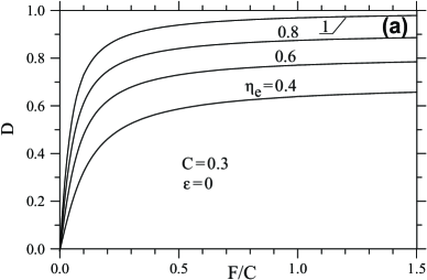
Figure 3: (a): Quantum feedback efficiency $D$ as a function of feedback strength $F$ for several values of quantum efficiency $\eta_{e}$ of the detection. (b): Maximum feedback efficiency $D_{max}$ (at large $F$) as a function of $\eta_{e}$. Dots show the Monte Carlo results for coupling ${\cal C}=0.1$, solid line corresponds to Eqs. (31)–(32), and dashed line shows the approximate formula (29).

The evolution of a non-pure qubit state with $\mbox{Re}\rho_{12}=0$ (since $\varepsilon=0$) can be parameterized as $\rho_{11}-\rho_{22}=P\cos\phi$, $\rho_{12}=iP(\sin\phi)/2$, where purity factor $P$ is between 0 and 1. Using Bayesian equations (3)–(4), we derive evolution equations for $P$ and $\phi$ (in Stratonovich form):

$$\dot{P}=\frac{\Delta I}{S_{I}}(1-P^{2})(\frac{\Delta I}{2}\,P\cos\phi+\xi)\cos\phi-\gamma P\sin^{2}\phi,$$ (25)

$$\dot{\phi}=2\frac{H_{fb}}{\hbar}-\frac{\sin\phi}{P}\frac{\Delta I}{S_{I}}\,(\frac{\Delta I}{2}\,P\cos\phi+\xi)-\gamma\frac{\sin 2\phi}{2}.$$ (26)

Sufficiently strong feedback (7) makes the phase $\phi$ arbitrarily close to the desired phase $\phi=\Omega_{0}t$ (mod $2\pi$), so the feedback efficiency is practically equal to the averaged purity factor: $D_{max}=\langle P\rangle$. To find $\langle P\rangle$ in the case of weak coupling ${\cal C}/\eta_{e}\ll 1$, let us perform first the averaging over oscillations and later the averaging over remaining slow fluctuations. It is easier to work with $P^{2}$ than with $P$, so we start with evolution equation for $P^{2}$ which is obtained from Eq. (25) as $dP^{2}/dt=2P\dot{P}$. It is easier to average $P^{2}$ over oscillation period using the Itô form Oksendal because the noise $\xi$ causes correlated noise of $\phi$, and only in the Itô form the average effect of the noise is zero. Using the standard rule Oksendal ; Kor-01 we translate the evolution equation for $P^{2}$ into Itô form:

$$\frac{dP^{2}}{dt}=\frac{(\Delta I)^{2}}{2S_{I}}(1-P^{2})(1-P^{2}\cos^{2}\phi)-2\gamma P^{2}\,\sin^{2}\phi$$

$$\hskip 14.22636pt+(2\Delta I/S_{I})P(1-P^{2})(\cos\phi)\,\xi\,;$$ (27)

then averaging over $\phi$ is trivial:

$$\frac{dP^{2}}{dt}=\frac{(\Delta I)^{2}}{2S_{I}}(1-P^{2})(1-\frac{P^{2}}{2})-\gamma P^{2}+\frac{\sqrt{2}\Delta I}{S_{I}}P(1-P^{2})\,\xi\,,$$ (28)

where $\xi(t)$ is now a different white noise but with the same spectral density $S_{\xi}=S_{I}$, so we do not change notation.

A simple estimate of $D_{max}$ can be obtained from Eq. (28) by neglecting the noise term and finding stationary value for $P$, which givesKorotkov-04

$$D_{max}\approx[1+1/2\eta_{e}-\sqrt{(1+1/2\eta_{e})^{2}-2}]^{1/2}.$$ (29)

If we do not neglect the noise term in Eq. (28), then $P^{2}$ fluctuates in time, and the stationary probability distribution $\sigma_{st}(P^{2})$ can be found from the Fokker-Planck-Kolmogorov equation similar to Eq. (15) (notice that varying diffusion coefficient comes inside the second derivative term) that leads to equation

$$[\gamma P^{2}-(1-P^{2})(1-P^{2}/2)(\Delta I)^{2}/2S_{I}]\sigma_{st}$$

$$+[(\Delta I)^{2}/2S_{I}]\frac{d}{d(P^{2})}[P^{2}(1-P^{2})^{2}\sigma_{st}]=0,$$ (30)

which has analytic solution $\sigma_{st}(P^{2})=N\,G(P^{2})$, where

$$G(P^{2})=(1-P^{2})^{-5/2}\exp\left[-\frac{\eta_{e}^{-1}-1}{2(1-P^{2})}\right]$$ (31)

and $N$ is the normalization factor. Stationary probability distribution for $P$ can be found as $\tilde{\sigma}_{st}(P)=2P\sigma_{st}(P^{2})$, and calculating the average $P$ gives us finally the feedback efficiency

$$D_{max}=\frac{\int_{0}^{1}P^{2}\,G(P^{2})\,dP}{\int_{0}^{1}P\,G(P^{2})\,dP}.$$ (32)

Figure 3(b) shows the dependence of the feedback efficiency $D_{max}$ on the effective quantum efficiency of the detector $\eta_{e}=(1+d_{e})^{-1}$. Solid line shows the analytical result (32), dashed line shows approximate formula (29), and the symbols show the numerical (Monte Carlo) results for $D_{max}$ (at sufficiently large $F$) for coupling ${\cal C}=0.1$. Notice that the lines for exact and approximate formulas are quite close to each other.

Since at finite detection efficiency $\eta_{e}$ the ensemble qubit dephasing is $\Gamma=\eta_{e}^{-1}(\Delta I)^{2}/4S_{I}$, the weak coupling condition requires ${\cal C}/\eta_{e}\lesssim 1$. As a result, the numerical results for ${\cal C}=0.1$ in Fig. 3 start to deviate (upwards) from the analytical result at $\eta_{e}\lesssim 0.03$. For larger ${\cal C}$ the deviation starts even at larger $\eta_{e}$. Numerical calculations also show that at ${\cal C}/\eta_{e}\gtrsim 3$ the average purity factor $\langle P\rangle$ has a noticeable dependence on the feedback factor $F$ ($\langle P\rangle$ decreases with increase of $F$), while at ${\cal C}/\eta_{e}\lesssim 1$ this dependence is negligible.

It is easy to see that in vicinity of the ideal case ($\eta_{e}\approx 1$) Eq. (29) gives linear approximation $D_{max}\approx(1+\eta_{e})/2\approx 1-d_{e}/2$ [exact solution (32) shows the same linear approximation]. This explains the corresponding numerical result of Ref. Ruskov-02, . In the opposite limiting case $\eta_{e}\ll 1$, Eq. (29) is reduced to $D_{max}\approx\sqrt{2\eta_{e}}$; the exact solution (32) has a similar dependence but with slightly different prefactor: $D_{max}\approx 1.25\sqrt{\eta_{e}}$. Because of the square root dependence, feedback efficiency is still significant even for large magnitude of qubit dephasing due to coupling with environment. For example, if coupling with dephasing environment is 10 times stronger than coupling with quantum-limited detector ($d_{e}=10$, $\eta_{e}=1/11$), then $D_{max}\simeq 0.36$, which is still a quite significant value for an experiment.

V Effect of $\varepsilon$ and $H$ deviation

In the ideal case we have assumed symmetric qubit ($\varepsilon=0$) and assumed that the exact value of tunneling parameter $H$ is used in the processor. In this Section we analyze what happens if the qubit parameters $\varepsilon$ and $H$ deviate from the “nominal” values $\varepsilon=0$ and $H=H_{0}$ assumed by an experimentalist and used in the processor. In this case the monitored value $\rho^{m}$ of the qubit density matrix differs from the actual value $\rho$; and because of the mistake in qubit monitoring, the feedback performance should obviously worsen. [Both $\rho(t)$ and $\rho^{m}(t)$ satisfy Eqs. (3)–(4) with the same detector output $I(t)$; however, “incorrect” parameters $\varepsilon=0$ and $H_{0}$ are used to calculate $\rho^{m}(t)$, while actual evolution $\rho(t)$ is governed by actual parameter values $\varepsilon$ and $H$.] The desired evolution is still $\rho_{11}^{d}=(1+\cos\Omega_{0}t)/2$, $\rho_{12}^{d}=i(\sin\Omega_{0}t)/2$ with $\Omega_{0}=2H_{0}/\hbar$, which is used in calculation of feedback efficiency $D$ [notice that in the definition of efficiency (10) $\rho^{d}(t)$ is multiplied by the actual density matrix $\rho(t)$, not the monitored value $\rho^{m}(t)$]. The controller is still given by Eq. (7) (we do not replace here $H$ by $H_{0}$ because this is more natural, for example, for control of the Cooper-pair-box qubit). Since the analytical analysis of the problem is quite complicated, in this Section we present only the numerical results of Monte Carlo simulations.

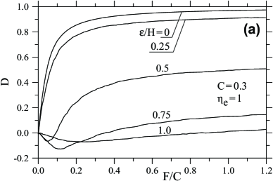
Figure 4: (a): Dependence $D(F)$ for several values of the qubit energy asymmetry $\varepsilon/H$ in the case when the processor and controller still assume $\varepsilon=0$. (b): Solid lines: maximized over $F$ feedback efficiency $D_{max}$ as a function of the asymmetry $\varepsilon/H$ for three values of coupling ${\cal C}=1$, 0.3, and 0.1. Dashed lines: the same curves for ${\cal C}=0.3$ and 0.1 drawn as functions of $\varepsilon/H\sqrt{\cal C}$. Dotted lines: dependence $D_{max}(\varepsilon/H)$ for the three values of $\cal C$ in the case when actual value of $\varepsilon$ is used in the processor, while the controller (7) is still designed for $\varepsilon=0$.

Let us start with deviation of $\varepsilon$ (while $H=H_{0}$). Figure 4(a) shows dependence $D(F)$ for ${\cal C}=0.3$ and several values of $\varepsilon$. One can see that for sufficiently large energy asymmetry $\varepsilon/H$ the feedback efficiency $D$ is negative at small $F$, while it is always positive at large $F$. For relatively small values of asymmetry ($|\varepsilon/H|\lesssim 1$) the dependence $D(F)$ apparently saturates at large $F$, while at larger asymmetry [$|\varepsilon/H|\gtrsim 1.5$; not shown in Fig. 4(a)] $D(F)$ has maximum at finite $F$. [We cannot exclude the possibility that even for small $\varepsilon/H$, $D(F)$ also has maximum, but it occurs at too large $F$ which cannot be analyzed by our code due to numerical problems.] Notice that the feedback efficiency is obviously insensitive to the sign of energy asymmetry: $D(-\varepsilon,H,{\cal C},F)=D(\varepsilon,H,{\cal C},F)$.

Solid lines in Fig. 4(b) show dependence of $D$ maximized over $F$, on energy asymmetry $\varepsilon/H$ for several values of the coupling ${\cal C}=0.1$, 0.3, and 1. One can see that at small $\varepsilon/H$ the dependence $D_{max}(\varepsilon/H)$ is parabolic (zero derivative at $\varepsilon=0$), which means that a small energy asymmetry of the qubit decreases the feedback efficiency very little. Zero derivative at $\varepsilon=0$ is a natural consequence of the symmetry $D_{max}(-\varepsilon/H)=D_{max}(\varepsilon/H)$ (because of this symmetry, we show only positive $\varepsilon/H$). As seen in Fig. 4(b), significant decrease of $D_{max}$ starts at smaller $\varepsilon/H$ for smaller coupling ${\cal C}$. Rescaling of the horizontal axis by $\sqrt{\cal C}$ makes the curves quite close to each other (see dashed lines in the Figure); however, we are not sure if the scaling $D_{max}(\varepsilon/H\sqrt{\cal C})$ is really exact at ${\cal C}\rightarrow 0$.

The dotted lines in Fig. 4(b) show dependence $D_{max}(\varepsilon/H)$ for a different situation, when the exact value of $\varepsilon$ is used in the processor, but the controller is still given by Eq. (7) designed for $\varepsilon=0$ [desired evolution is still given by Eq. (6) with $\Omega_{0}=2H/\hbar$]. One can see that exact monitoring of the qubit significantly improves the feedback efficiency compared with the case considered above; however, the feedback efficiency still decreases with energy asymmetry because the desired evolution (6) cannot be achieved at nonzero $\varepsilon/H$ and also because of non-optimal controller still designed for $\varepsilon=0$. (Some apparent dependence of the dotted lines on ${\cal C}$ even at ${\cal C}\ll 1$ is possibly due to numerical problems of the code which does not work really well at ${\cal C}\lesssim 0.1$.)

To analyze the effect of the deviation of the parameter $H$ from the value $H_{0}$ used in the processor, we assume perfect energy symmetry, $\varepsilon=0$. Figure 5(a) shows the dependence $D(F)$ for ${\cal C}=0.3$ and several values of the relative deviation $(H-H_{0})/H$ (we show only the curves for positive deviation; the curves for negative deviation are similar). We see that the effect of $H$ deviation is qualitatively similar to the effect of energy asymmetry [compare Figs. 4(a) and 5(a)]. At large $F$ the dependence $D(F)$ saturates. Figure 5(b) shows the value $D_{max}$ maximized over $F$ as a function of the relative deviation $(H-H_{0})/H$ for several values of the coupling ${\cal C}$. One can see that the dependence is almost symmetric for positive and negative deviation, and is parabolic at small deviation similar to the case of nonzero $\varepsilon$ discussed above. Also similar is the fact that weaker coupling $\cal C$ requires smaller deviation of $H$ for the same value of feedback efficiency. However, the scaling with ${\cal C}$ is now different: the curves become close to each other if $D_{max}$ is plotted as a function of $(H-H_{0})/H{\cal C}$ [see dashed lines in Fig. 5(b)]. The different scaling is a natural consequence of the fact that small change of $\Omega=\sqrt{4H^{2}+\varepsilon^{2}}/\hbar$ is linear in $H$ deviation but quadratic in $\varepsilon$. The results presented in Figs. 4(b) and 5(b) can be crudely interpreted in the following way: $D_{max}$ decreases significantly when the Rabi frequency change due to parameter deviations ($\Delta\Omega=2\Delta H/\hbar$ or $\Delta\Omega\approx\varepsilon^{2}/4H\hbar$) becomes comparable to the “measurement rate” $(\Delta I)^{2}/4S_{I}$. [Notice that if the horizontal axis in Fig. 5(b) was chosen as $(H-H_{0})/H_{0}$, the curves would be somewhat more asymmetric, the asymmetry being more significant at larger $\cal C$.]

Figure 5: Effect of the deviation of the qubit parameter $H$ from the value $H_{0}$ assumed in the processor. (a): Dependence $D(F)$ for several values of the relative deviation $(H-H_{0})/H$. (b): Solid lines: optimized over $F$ feedback efficiency $D_{max}$ as function of the deviation $(H-H_{0})/H$ for coupling ${\cal C}=1$, 0.3, and 0.1. Dashed lines: the same curves for ${\cal C}=0.3$ and 0.1 drawn as functions of $(H-H_{0})/H{\cal C}$.

Concluding the discussion of $\varepsilon$ and $H$ deviations, let us mention that the main practical conclusion of the analysis is that the feedback operation is robust against small unknown deviations of the qubit parameters.

VI Feedback control of a qubit with energy asymmetry $\varepsilon$

In this Section we analyze the case of a qubit with finite energy asymmetry $\varepsilon$ (“asymmetric qubit”). In contrast to the problem considered in the previous Section, in which nonzero $\varepsilon$ was treated as an unwanted deviation from the perfect zero value (therefore, finite $\varepsilon$ was just worsening the feedback designed for $\varepsilon=0$), now we try to design and analyze a different feedback (different controller) which goal is to maintain the free oscillations of a qubit with $\varepsilon\neq 0$ (so, now effect of nonzero $\varepsilon$ is what we also want to protect from decoherence). Hence, the desired evolution $\rho^{d}(t)$ is no longer given by Eq. (6).

Before choosing the desired evolution, let us mention that the qubit asymmetry leads to one more degree of freedom on the Bloch sphere. In case of $\varepsilon=0$, a pure qubit state was characterized only by the phase $\phi$ [see Eq. (11)] because the real part of $\rho_{12}$ was vanishing in the course of measurement, so the evolution was within the plane of “zero longitude meridian”. For an asymmetric qubit, a naturally preferable plane of oscillations on the Bloch sphere no longer exists; in particular a weak measurement leads to a slow fluctuation of the “slanted” plane of free qubit oscillations (Fig. 6). The simulations show that without feedback the pure-state qubit evolution is to some extent confined between the two slanted planes passing through the “north pole” ($\rho_{11}=1$) and “south pole” ($\rho_{22}=1$), with the probability about 0.6 of being between the two planes for small $\cal C$ and $|\varepsilon/H|\lesssim 1$.

Let us choose the desired qubit evolution as a free evolution starting from the north pole:

$$\rho_{11}^{d}(t)=\frac{2H^{2}+\varepsilon^{2}+2H^{2}\cos\Omega t}{4H^{2}+\varepsilon^{2}}$$

$$\hskip 28.45274pt=1+\frac{1}{2}\cos^{2}\alpha\,(\cos\Omega t-1),$$ (33)

$$\rho_{12}^{d}(t)=\frac{\varepsilon H(\cos\Omega t-1)}{4H^{2}+\varepsilon^{2}}+\frac{iH\sin\Omega t}{(4H^{2}+\varepsilon^{2})^{1/2}}$$

$$\hskip 28.45274pt=\frac{\cos\alpha}{2}\,[\sin\alpha(\cos\Omega t-1)+i\sin\Omega t].$$ (34)

where $\Omega=\sqrt{4H^{2}+\varepsilon^{2}}/\hbar$ and $\alpha=\mbox{atan}(\varepsilon/2H)$. An interesting question is whether the quantum feedback can keep the qubit evolution close to the desired path (33)–(34) or not.

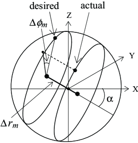
Figure 6: Illustration of the qubit evolution on the Bloch sphere. For an asymmetric qubit ($\varepsilon\neq 0$) the free evolution is a rotation about a slanted (by angle $\alpha$) axis. The difference between actual and desired qubit states (both are pure states) is characterized by the distance $\Delta r_{m}$ between the corresponding slanted planes and the angle $\Delta\phi_{m}$ within the slanted plane (after projection).

The old controller (7) is obviously not good for this purpose, so we need to design a new one. [Notice that the qubit density matrix is monitored exactly, $\rho^{m}(t)=\rho(t)$, because all the parameters are assumed to be known exactly and because as discussed in Section II we assume infinite signal bandwidth.] As the first step, we characterize the deviation of the monitored qubit state $\rho^{m}(t)$ from the desired state $\rho^{d}(t)$ by two magnitudes (see Fig. 6): by the distance $\Delta r_{m}$ between two parallel slanted planes containing the monitored and desired states (the planes are slanted by angle $-\alpha$) and by the angular difference $\Delta\phi_{m}$ between points $\rho^{m}$ and $\rho^{d}$ projected onto the slanted plane. The corresponding formulas are a little lengthy but straightforward. For the distance deviation $\Delta r_{m}=r_{m}-r_{d}$ we calculate the distances $r_{m}$ and $r_{d}$ of the planes from the origin as the scalar products of the vector $(\cos\alpha,0,-\sin\alpha)$ orthogonal to the planes and the Bloch vectors $(2\mbox{Re}\rho_{12},2\mbox{Im}\rho_{12},\rho_{11}-\rho_{22})$ for the states $\rho^{m}$ and $\rho^{d}$, correspondingly:

$$r_{m}=2\mbox{Re}\rho_{12}^{m}\cos\alpha-(\rho_{11}^{m}-\rho_{22}^{m})\sin\alpha$$ (35)

and similar for $r_{d}$; it easy to see from Eqs. (33)–(34) that $r_{d}=-\sin\alpha$. For the phase difference $\Delta\phi_{m}=\phi_{m}-\phi_{d}$ (mod $2\pi$, $|\Delta\phi_{m}|\leq\pi$) we use equation

$$\mbox{tan}\,\phi_{m}=\frac{2\mbox{Im}\rho_{12}^{m}}{2\mbox{Re}\rho_{12}^{m}\sin\alpha+(\rho_{11}^{m}-\rho_{22}^{m})\cos\alpha}\,$$ (36)

[extra $\pi$-shift of $\phi_{m}$ is added when the denominator is negative as in Eq. (9)]; a similar equation for $\rho^{d}$ defined by Eqs. (33)–(34) obviously gives $\phi_{d}=\Omega t$ (mod $2\pi$). Notice that in the case $\varepsilon=0$ (so that $\alpha=0$) we recover the previous definition (9) of $\Delta\phi_{m}$, while $\Delta r_{m}=0$.

Limiting ourselves by the feedback control of the qubit parameter $H$ only, we designed and analyzed the following controller:

$$\Delta H_{fb}=-FH\Delta\phi_{m}-F_{r}H\sin\phi_{m}\Delta r_{m}.$$ (37)

The first term in this expression is the same as in the previous controller (7) and is supposed to reduce the in-plane phase difference $\Delta\phi_{m}$ by changing the oscillation frequency, while the second term is supposed to reduce the inter-plane distance $\Delta r_{m}$. The idea is that the change of $H_{fb}=H+\Delta H_{fb}$ affects the angle of the slanted plane of oscillations, and when it is done periodically in phase with the oscillations (due to the factor $\sin\phi_{m}$) the inter-plane distance can be gradually reduced.

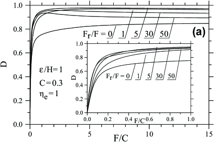
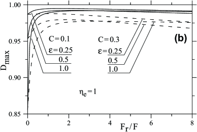
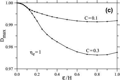
Figure 7: Feedback efficiency for an energy-asymmetric qubit ($\varepsilon\neq 0$). (a): Dependence $D(F)$ for several values of the ratio $F_{r}/F$. Inset shows the same curves at small $F$. (b): Optimized over $F$ feedback efficiency $D_{max}$ as a function of $F_{r}/F$ for several values of qubit asymmetry $\varepsilon/H$ and two values of coupling ${\cal C}$. (c): Feedback efficiency $D_{max}$ optimized over both $F$ and $F_{r}$, as a function of asymmetry $\varepsilon/H$ for two values of ${\cal C}$. Dots show numerical results while the lines just connect the dots.

Numerical calculations show that this idea works really well. Figure 7(a) shows the dependence $D(F)$ for several values of the ratio $F_{r}/F$ using as an example parameters $\varepsilon/H=1$, ${\cal C}=0.3$, and $\eta_{e}=1$. One can see that non-zero $F_{r}$ can significantly improve the feedback efficiency $D$. While at $F_{r}=0$ the dependence $D(F)$ saturates at large $F$, at non-zero $F_{r}$ the efficiency $D$ has maximum at finite $F$.

Figure 7(b) shows the optimized over $F$ efficiency $D_{max}$ as function of the ratio $F_{r}/F$ for couplings ${\cal C}=0.3$ and 0.1, and three values of energy asymmetry $\varepsilon/H$. One can see that each curve has maximum at some value of $F_{r}/F$. Notice also that at zero $F_{r}$, the curves for different coupling ${\cal C}$ practically coincide, while at finite $F_{r}/F$ their behavior significantly depends on ${\cal C}$, with larger $D_{max}$ at smaller coupling.

In Fig. 7(c) we show the feedback efficiency $D_{max}$ optimized over both $F$ and $F_{r}$ as function of energy asymmetry $\varepsilon/H$ for two values of the coupling ${\cal C}$. As we see, finite asymmetry $\varepsilon/H$ prevents efficiency $D_{max}$ from reaching 100%. However, the difference $1-D_{max}$ decreases with decrease of coupling ${\cal C}$, crudely proportional to ${\cal C}$ (except the region of small $\varepsilon/H$, where the accuracy of our calculations is possibly insufficient to distinguish the curves; unfortunately, there is no simple way to estimate the calculation accuracy). Therefore, we guess that for any asymmetry $\varepsilon/H$, the feedback efficiency $D_{max}$ reaches 100% in the limit of small coupling ${\cal C}\rightarrow 0$. (We cannot check this conjecture numerically because our code does not work well at ${\cal C}<0.1$.)

Limiting the feedback control by the control of the parameter $H$ only, is not quite natural for the asymmetric qubit (though it is simpler from the experimental point of view). We have also performed a preliminary analysis of a simultaneous control of both $H$ and $\varepsilon$. We have considered the case when Eq. (37) is used for $H$-feedback while a similar equation (with $H$ replaced by $\varepsilon$) is used for simultaneous control of $\varepsilon$. Even though we have not performed detailed optimization, we have obtained larger values of $D_{max}$ than those presented in Figs. 7(b) and 7(c). This shows that additional feedback control of the qubit parameter $\varepsilon$ really improves the feedback efficiency.

Concluding this Section let us mention that its main result is the possibility of a very efficient feedback control of an asymmetric qubit. This can be done even using the control of the parameter $H$ only, while simultaneous control of $\varepsilon$ further improves the operation of the feedback.

VII Conclusion

In this paper we have analyzed the quantum feedback control of a single qubit, designed to maintain perfect (or close to perfect) Rabi oscillations for arbitrarily long time. We have considered “Bayesian” feedback Ruskov-02 which requires a “processor” (see Fig. 1) solving quantum Bayesian equations to monitor the qubit state evolution via continuous output signal from the detector (QPC or SET) weakly coupled to the qubit. After comparing the randomly evolving (due to quantum back-action) monitored qubit state $\rho^{m}$ with the desired state $\rho^{d}$, the qubit tunneling parameter $H$ is being slightly changed in order to reduce the difference between the states. For simplicity we have assumed infinite bandwidth of the (noisy) detector signal and neglected the time delay in the feedback loop.

The analysis in Section III shows that in the ideal case the efficiency $D$ of the quantum feedback can be made arbitrarily close to 100% by increasing the strength of the feedback control [characterized by parameter $F$ in Eq. (7)]. It is important to mention that $F$ scales with the coupling ${\cal C}$ between qubit and detector; therefore in the realistic case of weak coupling ${\cal C}\ll 1$, the parameter $F$ and consequently the relative change of the qubit parameter $H$ remain small. The efficient operation of the feedback loop is achieved at $F/{\cal C}\gg 1$ [see Eq. (16)]; in this case the qubit evolution becomes almost perfectly sinusoidal [Eqs. (20) and (21)], while the spectral density of the detector current [Eq. (24)] contains the $\delta$-function peak at Rabi frequency $\Omega_{0}$ with the integral $(\Delta I)^{2}/8$ (as would be expected for the synchronized classical sinusoidal oscillations in the qubit) and also a narrow peak around $\Omega_{0}$ with the same integral. The total integral under the peaks is thus $(\Delta I)^{2}/4$, which exceeds the limit for a classically interpretable process.Ruskov-05

The feedback performance worsens in the case of a nonideal detector and/or presence of dephasing environment. This case is considered in Section IV. We have obtained an analytical formula [Eqs. (31)–(32)] for the maximum feedback efficiency $D_{max}$ confirmed by Monte Carlo simulations. It gives $D_{max}\approx(1+\eta_{e})/2$ in almost perfect case when the effective detection efficiency $\eta_{e}$ is close to unity, and $D_{max}\approx 1.25\sqrt{\eta_{e}}$ when $\eta_{e}\ll 1$.

In Section V we have analyzed numerically the decrease of the feedback efficiency in the case when actual qubit parameters $\varepsilon$ and $H$ differ from the assumed (in the processor and controller) parameters $\varepsilon=0$ and $H=H_{0}$ (otherwise the case is ideal). We have found that for small deviations the efficiency $D_{max}$ decreases relatively slowly (with zero derivative at vanishing deviation), so that, for example, $D_{max}\geq 0.95$ is possible for $|\varepsilon/H_{0}|<0.5\sqrt{\cal C}$ and $|H/H_{0}-1|<0.03\,{\cal C}$. This shows that the quantum feedback is robust against small deviations of the qubit parameters.

In Section VI we have analyzed the feedback control of a qubit with finite energy asymmetry $\varepsilon$, so that the desired evolution trajectory is along a slanted circle on the Bloch sphere. Despite the control problem becomes two-dimensional in this case even for a pure state, we have shown that efficient feedback is still possible using only one controlled parameter $H$ and properly designed algorithm (controller).

The Bayesian quantum feedback of a solid-state qubit analyzed in this paper is not yet realizable experimentally at the present-day level of technology. Even much simpler quadrature-based quantum feedback Korotkov-04 is still a big experimental challenge. However, a rapid progress in experiments with solid-state qubit and also recent realization of quantum feedback in optics Geremia allow us to believe that the analysis performed in this paper will eventually be experimentally relevant. In this paper we have not considered two more effects quite important for the operation of the Bayesian quantum feedback: finite signal bandwidth and time delay in the loop. These effects will be a subject of a separate publication.

The work was supported by NSA and ARDA under ARO grant W911NF-04-1-0204.

References

- (1) H. M. Wiseman and G. J. Milburn, Phys. Rev. Lett. 70, 548 (1993); Phys. Rev. A 49, 1350 (1994).
- (2) P. Tombesi and D. Vitali, Phys. Rev. A 51, 4913 (1995); M. Fortunato, J. M. Raimond, P. Tombesi, and D. Vitali, Phys. Rev. A 60, 1687 (1999).
- (3) H. F. Hofmann, G. Mahler, and O. Hess, Phys. Rev. A 57, 4877 (1998).
- (4) J. Wang and H. M. Wiseman, Phys. Rev. A 64, 063810 (2001); J. Wang, H. M. Wiseman, and G. J. Milburn, quant-ph/0011074.
- (5) A. C. Doherty and K. Jacobs, Phys. Rev. A 60, 2700 (1999).
- (6) J. H. Shapiro, G. Saplakoglu, S. T. Ho, P. Kumar, B. E. A. Saleh, and M. C. Teich, J. Opt. Soc. Am. B 4, 1604 (1987).
- (7) Y. Yamamoto, N. Imoto, and S. Machida, Phys. Rev. A 33, 3243 (1986); H. A. Haus and Y. Yamamoto, Phys. Rev. A 34, 270 (1986).
- (8) C. M. Caves and G. J. Milburn, Phys. Rev. A 36, 5543, (1987).
- (9) H. M. Wiseman, Phys. Rev. A 49, 2133 (1994).
- (10) A. C. Doherty, S. Habib, K. Jacobs, H. Mabuchi, and S. M. Tan, Phys. Rev. A 62, 012105 (2000); A. C. Doherty, K. Jacobs, and G. Jungman, Phys. Rev. A 63, 062306 (2001).
- (11) JM Geremia, J. K. Stockton, and H. Mabuchi, Science 304, 270 (2004); M. A. Armen, J. K. Au, J. K. Stockton, A. C. Doherty, and H. Mabuchi, Phys. Rev. Lett. 89, 133602 (2002).
- (12) R. Ruskov and A. N. Korotkov, Phys. Rev. B 66, 041401(R) (2002).
- (13) R. Ruskov, Q. Zhang, and A. N. Korotkov, Proceedinds of SPIE, vol. 5436, p. 162 (2004); Proceedings of 42th IEEE conference on Decision and Control (Maui, HI, 2003), p. 4185.
- (14) A. N. Korotkov, Phys. Rev. B 71, 201305(R) (2005).
- (15) A. Hopkins, K. Jacobs, S. Habib, and K. Schwab, Phys. Rev. B 68, 235328 (2003).
- (16) R. Ruskov, K. Schwab, and A. N. Korotkov, IEEE Trans. Nanotech. 4, 132 (1995); Phys. Rev. B 71, 235407 (2005).
- (17) J. von Neumann, Mathematical Foundations of Quantum Mechanics (Princeton Univ. Press, Princeton, 1955).
- (18) A. O. Caldeira and A. J. Leggett, Ann. Phys. (N.Y.) 149, 374 (1983); W. H. Zurek, Phys. Today 44 (10), 36 (1991).
- (19) M. B. Mensky, Phys. Rev. D 20, 384 (1979).
- (20) N. Gisin, Phys. Rev. Lett. 52, 1657 (1984).
- (21) C. M. Caves, Phys. Rev. D 33, 1643 (1986).
- (22) H. J. Carmichael, An open system approach to quantum optics, Lecture notes in physics (Springer, Berlin, 1993).
- (23) M. B. Plenio and P. L. Knight, Rev. Mod. Phys. 70, 101 (1998).
- (24) A. N. Korotkov, Phys. Rev. B 60, 5737 (1999).
- (25) A. N. Korotkov, Phys. Rev. B 63, 115403 (2001).
- (26) A. N. Korotkov, in Quantum noise in mesoscopic physics, edited by Yu. V. Nazarov (Kluwer, Netherlands, 2003), p. 205 (cond-mat/0209629).
- (27) H.-S. Goan, G. J. Milburn, H. M. Wiseman, and H. B. Sun, Phys. Rev. B 63, 125326 (2001).
- (28) H.-S. Goan and G. J. Milburn, Phys. Rev. B 64, 235307 (2001).
- (29) N. P. Oxtoby, H. B. Sun, and H. M. Wiseman, J. Phys.: Condens. Matter 15, 8055 (2003).
- (30) W. Feller, An Introduction to Probability Theory and Its Applications, v. 1 (Wiley, NY, 1968).
- (31) S. A. Gurvitz, Phys. Rev. B 56, 15215 (1997).
- (32) A. Shnirman and G. Schön, Phys. Rev. B 57, 15400 (1998); Y. Makhlin, G. Schön, and A. Shnirman, Rev. Mod. Phys. 73, 357 (2001).
- (33) D. V. Averin, in Exploring the quantum/classical frontier, ed. by J. R. Friedman and S. Han (Nova Science Publishers, NY, 2003), p. 447.
- (34) S. Pilgram and M. Büttiker, Phys. Rev. Lett. 89, 200401 (2002); A. N. Jordan and M. Büttiker, Phys. Rev. B 71, 125333 (2005).
- (35) A. A. Clerk, S. M. Girvin, and A. D. Stone, Phys. Rev. B 67, 165324 (2003).
- (36) It may be more meaningful to define as a negative real number to have a natural form for the qubit ground state; however, we prefer the choice of positive that can always be done by changing the phase of one of the localized states.
- (37) A. N. Korotkov, Phys. Rev. B 63, 085312 (2001).
- (38) N. P. Oxtoby, P. Warszawski, H. M. Wiseman, H.-B. Sun, and R. E. S. Polkinghorne, cond-mat/0401204.
- (39) R. Jozsa, J. Modern Optics 41, 2315 (1994).
- (40) B.Øksendal, Stochastic differential equations (Springer, Berlin, 1998).
- (41) R. Ruskov, A. N. Korotkov, and A. Mizel, cond-mat/0505094.