First Passage Time Densities in Non-Markovian Models with Subthreshold Oscillations

Abstract

Motivated by the dynamics of resonant neurons we consider a differentiable, non-Markovian random process $x(t)$ and particularly the time after which it will reach a certain level $x_{b}$. The probability density of this first passage time is expressed as infinite series of integrals over joint probability densities of $x$ and its velocity $\dot{x}$. Approximating higher order terms of this series through the lower order ones leads to closed expressions in the cases of vanishing and moderate correlations between subsequent crossings of $x_{b}$. For a linear oscillator driven by white or coloured Gaussian noise, which models a resonant neuron, we show that these approximations reproduce the complex structures of the first passage time densities characteristic for the underdamped dynamics, where Markovian approximations (giving monotonous first passage time distribution) fail.

1 Introduction

The first passage time (FPT) of a stochastic process $x(t)$ starting at $t=0$ from a given initial value within an a priory prescribed domain $\Omega$ of its state space is the time $T$ when $x(t)$ leaves $\Omega$ for the first time. This concept was originally introduced by E. Schrödinger when discussing behaviour of Brownian particles in external fields [1]. A large variety of problems ranging from noise in vacuum tubes, chemical reactions and nucleation [2] to stochastic resonance [3], behaviour of neurons [4], and risk management in finance [5] can be reduced to FPT problems.

We will assign ${\cal F}(T)$ to be the flux through the boundary of $\Omega$ at time $T$, i.e. the probability density of the first passage time. Approaches to find ${\cal F}(T)$ are typically based either on the Fokker-Planck equation with an absorbing boundary [6] or on the renewal theory [7]. Despite the long history, explicit expressions for the FPT density are known only for a few cases. These include overdamped particles in the force free case, with time-independent constant forces and linear forces under influence of white noise [4, 8, 9, 10], as well as the case of a constant force under coloured noise [11]. Reasonable approximations exist for a few nonlinear forces [12, 13].

If the relaxation time $\tau_{rel}$ of the system to a quasistationary distribution in $\Omega$ is much smaller than the typical first passage time, the escape from $\Omega$ occurs from this quasiequilibrium state independent of the initial condition. Escapes occur with a constant rate inversely proportional to the mean FPT. This is the case for many chemical reactions and nucleation processes [2] as well as for the leaky integrate-and-fire model of a neuron [14]. On times $T$ exceeding $\tau_{rel}$ the FPT probability density ${\cal F}(T)$ decays exponentially.

If the scale separation between relaxation and escape times does not hold, the dependence on the initial conditions gets crucial [20]. This situation is found in resonant neurons [15, 16, 17, 18, 19] where $x$, here the voltage variable, exhibits damped subthreshold oscillations around the rest state being the attractor for deterministic dynamics of the system. If $x(t)$ exceeds the excitation threshold $x_{b}$, a new spike begins. After spiking the voltage is reset to a fixed value $x_{0}$ far from the rest state and can reach $x_{b}$ again prior to relaxation. ${\cal F}(T)$ giving the probability density function (PDF) of intervals between two consecutive spikes strongly deviates from an exponential. This is the situation we have in mind when developing the approach for obtaining ${\cal F}(T)$ for a non-Markovian differentiable random processes $x(t)$ starting for $t=0$ at $x(0)=x_{0}<x_{b}$.

Our approach is based on a series expansion for ${\cal F}(T)$ which is known for several decades [23]. But it was never used for explicit calculations. The approach is based on the theory of level crossings originally put forward by S.O. Rice [21]. A generalisation of his approach (based on what is called the Wiener-Rice series [22]) was used by Stratonovich to estimate the mean time spent by a stochastic process above the given level $x_{b}$ [10]. The exact expression for ${\cal F}(T)$ is analogous to the Wiener-Rice series, but corresponds to the case when the initial value $x(0)$ differs from the threshold $x_{b}$.

We first give an elementary derivation of this result and show then how this series can be used to obtain analytical expressions based on decoupling approximations. Explicit calculations are performed for an underdamped harmonic oscillator driven by white or coloured Gaussian noise, i.e. for a resonate-and-fire neuron with subthreshold oscillations and reset. The linearity of the model simplifies calculations but is not crucial for the approach.

2 Level crossings and first passage times

Let us first discuss the probability $n_{1}(x_{b},t|\{x_{0}\},0)dt$ that a differentiable random process $x(t)$ starting from a fully defined initial condition $\{x_{0}\}=\{x(0),\dot{x}(0),...\}$ (corresponding to its Markovian embedding) with $x(0)<x_{b}$ crosses the level $x_{b}$ between $t$ and $t+dt$ with positive velocity $v(t)=\dot{x}(t)>0$ (i.e. performs an upcrossing). The upcrossing can only occur for such $x(t)$ that $x_{b}-vdt<x(t)<x_{b}$. The probability of this is $\int_{x_{b}-vdt}^{x_{b}}P(x,v,t|\{x_{0}\},0)dx=|v|P(x_{b},v,t|\{x_{0}\},0)dt$, where $P(x,v,t|\{x_{0}\},0)$ is the joint PDF for $x$ and $v$ under given initial conditions. Integration over all $v>0$ then gives $n_{1}(x_{b},t|\{x_{0}\},0)=\int_{0}^{\infty}vP(x_{b},v,t|\{x_{0}\},0)dv$. The joint probabilities for multiple upcrossings $n_{p}(t_{p},\dots,t_{1})dt_{p}\dots dt_{1}$ in each of $p$ time intervals $(t_{1},t_{1}+dt_{1}),\dots(t_{p},t_{p}+dt_{p})$ follow in the same way:

$$n_{p}(t_{p},\dots,t_{1})=\int_{0}^{\infty}dv_{p}\dots\int_{0}^{\infty}dv_{1}v_{p}\dots v_{1}P(x_{b},v_{p},t_{p};\dots;x_{b},v_{1},t_{1}|\{x_{0}\},0).$$ (1)

The initial conditions and $x_{b}$ will be omitted in what follows.

The function ${\cal F}(T)$ is given by the fraction of all trajectories $x(t)$ which perform the first upcrossing of $x_{b}$ at time $T$. All such trajectories are accounted for in $n_{1}(T)$. However, $n_{1}(T)$ also considers trajectories which might have an earlier upcrossing at some $0<t_{1}<T$. Since they should not contribute to ${\cal F}(T)$, their fraction should be subtracted from $n_{1}(T)$ by taking $n_{1}(T)-\int_{0}^{T}n_{2}(T,t_{1})dt_{1}$. This excludes all trajectories which cross $x_{b}$ exactly twice until $T$. However the trajectories crossing $x_{b}$ three times, i.e at $T$ and at two earlier moments $t_{i}<T,(i=1,2)$, are not correctly accounted. Each such trajectory is added once in $n_{1}(T)$, but subtracted two times in $\int_{0}^{T}n_{2}(T,t_{1})dt_{1}$, since this term accounts for the pairs of upcrossings at $(T,t_{i})$ with $i=1,2$. To account for this we have to add once the amount of trajectories with three upcrossings again: $n_{1}(T)-\int_{0}^{T}n_{2}(T,t_{1})dt_{1}+\frac{1}{2!}\int_{0}^{T}\int_{0}^{T}n_{3}(T,t_{2},t_{1})dt_{2}dt_{1}$ (the factor $1/2!$ in the last term accounts for permutations of $t_{i}$).

Generally, if a trajectory crosses $x_{b}$ at time $T$ and at $N$ earlier times $t_{i}<T$, $i=1\dots N$, then in $\frac{1}{p!}\int\dots\int n_{p+1}(T,t_{p},\dots,t_{1})dt_{p}\dots dt_{1}$ it is accounted for exactly $C_{N}^{p}$ times ($C_{N}^{p}$ stands for the number of combinations). Note, that $\sum_{p=0}^{N}(-1)^{p}C_{N}^{p}=(1-1)^{N}=0$. Thus in the alternating sum of this kind containing $N+1$ terms, all trajectories crossing $x_{b}$ at time $T$ and having $1,2,\dots N$ additional upcrossings are excluded. Extending the sum to infinity we exclude all superfluous trajectories. Only trajectories remain for which the upcrossing at time $T$ was the first one. Thus the expression for the first passage time probability density reads:

$${\cal F}(T)=\sum_{p=0}^{\infty}\frac{(-1)^{p}}{p!}\int_{0}^{T}dt_{p}\dots\int_{0}^{T}dt_{1}n_{p+1}(T,t_{p},\dots,t_{1}).$$ (2)

In Ref. [7, 10] it was shown that ${\cal F}(T)$ can be equivalently expressed in terms of the correlation functions between upcrossings (cross-cumulants) $g_{p}(t_{p},\dots,t_{1})$. They are related to the joint densities $n_{p}(t_{p},\dots,t_{1})$ via

$$g_{1}(t_{1})=n_{1}(t_{1}),$$

$$g_{2}(t_{2},t_{1})=n_{2}(t_{2},t_{1})-n_{1}(t_{1})n_{1}(t_{2}),$$ (3)

$$g_{3}(t_{3},t_{2},t_{1})=n_{3}(t_{3},t_{2},t_{1})-3\{n_{1}(t_{1})n_{2}(t_{3},t_{2})\}_{s}+2n_{1}(t_{1})n_{1}(t_{2})n_{1}(t_{3}),\qquad\dots.$$

Here $\{\dots\}_{s}$ denotes the symmetrisation of the expression in the brackets with respect to all permutations of its arguments. The expression for ${\cal F}(T)$ in terms of correlation functions reads [10]:

$${\cal F}(T)=S^{\prime}(T)e^{-S(T)}$$ (4)

with

$$S(T)=-\sum_{p=1}^{\infty}\frac{(-1)^{p}}{p!}\int_{0}^{T}dt_{p}\dots\int_{0}^{T}dt_{1}g_{p}(t_{p},\dots,t_{1}).$$ (5)

The function $S^{\prime}(T)$ can be interpreted as a the time-dependent escape rate.

We emphasise that expressions eqs.(2),(4) and (5) do hold for all differentiable random processes (ones whose velocity $v(t)$ is defined at any time).

3 Decoupling approximations for the FPT density

Dealing with infinite series useful approximations can either be based on the truncation of the series after several first terms calculated exactly, or on expressing the higher order terms approximately through the lower order ones what might lead to a closed analytical form. Truncation approximations for eq.(2) are not normalised and hold on short time scales only diverging at longer times (due to the miscount of trajectories with several upcrossings). We discuss here the approximations of the second type which are normalised and can be used in the whole time domain. Each such approximation is based on a subsummation in eq.(5) for $S(T)$. Note, only expressions guaranteeing positive rates $S(T)$ are allowed.

The simplest approximation is based on neglecting all terms in eq.(5) except for the first one. It leads to

$$S(T)=\int_{0}^{T}n_{1}(t)dt,$$ (6)

where $n_{1}(t)$ is given by eq.(1) with $p=1$. This corresponds to neglecting all correlations between upcrossings of the level $x_{b}$, i.e. to factorisation of $n_{p+1}(T,t_{p},\dots,t_{1})$ into a product of one-point densities $n_{1}(T)n_{1}(t_{p})\dots n_{1}(t_{1})$ in eq.(2). Then the series, eq.(2) sums up into ${\cal F}(T)\approx n_{1}(T)\exp\left(-\int_{0}^{T}n_{1}(t)dt\right)$, which is equivalent to eq.(6). The approximation will be refereed to as a Hertz approximation since the form of ${\cal F}(T)$ resembles the Hertz distribution [24].

The second order approximation expresses all higher order correlation functions through the first and the second ones. It was used by Stratonovich [10] in the context of peak duration. The first and the second correlation functions are taken exactly, and the higher ones are approximated by the combinations of these two. For $p\geq 2$ one thus has

$$g_{p}(t_{p},\dots,t_{1})\approx(-1)^{p-1}(p-1)!n_{1}(t_{p})\dots n_{1}(t_{1})\{R(t_{1},t_{2})R(t_{1},t_{3})\dots R(t_{1},t_{p})\}_{s}$$ (7)

with the correlation coefficient

$$R(t_{i},t_{j})=1-\frac{n_{2}(t_{i},t_{j})}{n_{1}(t_{i})n_{1}(t_{j})}.$$ (8)

The correlation coefficient $R(t_{1},t_{2})$ is equal to unity for $t_{1}=t_{2}$ and vanishes for large values of $|t_{1}-t_{2}|$. Substitution of eq.(7) into eq.(5) delivers then the Stratonovich approximation for ${\cal F}(T)$ with the time-dependent escape rate being

$$S(T)=-\int_{0}^{T}n_{1}(t)\frac{\ln\left[1-\int_{0}^{T}R(t,t^{\prime})n_{1}(t^{\prime})dt^{\prime}\right]}{\int_{0}^{T}R(t,t^{\prime})n_{1}(t^{\prime})dt^{\prime}}dt.$$ (9)

4 Noise driven harmonic oscillator

Let us now illustrate the method by applying it to the coordinate $x(t)$ of a harmonic oscillator driven by a Gaussian noise $\eta(t)$

$$\dot{x}=v,\quad\dot{v}=-\gamma v-\omega_{0}^{2}x+\eta(t).$$ (10)

Two cases will be considered: (i) white noise, $\eta(t)=\sqrt{2D}\xi(t)$, and (ii) Ornstein-Uhlenbeck noise, $\dot{\eta}=-\tau^{-1}\eta+\sqrt{2D}\tau^{-1}\xi(t)$, with $\xi(t)$ being white Gaussian noise of intensity $1$. Eq.(10) with boundary at $x_{b}$ and reset at $x(0)=x_{0},\dot{x}(0)=v_{0}$ is relevant for a modelling of neuronal dynamics. In the underdamped regime $\gamma<2\omega_{0}$ it describes an excitable dynamics with damped subthreshold oscillations characteristic for resonant neurons [15, 16, 17, 18, 19]. In the overdamped regime $\gamma>2\omega_{0}$ it describes the behaviour of nonresonant neurons [15, 25]. In our calculations we fix $\omega_{0}=1$, take initial conditions to be $x_{0}=-1,v_{0}=0$, and set the absorbing boundary at the threshold $x_{b}=1$.

Our basic model has an advantage that all transition probability densities in eq.(1) are Gaussian and can be expressed through the correlation functions of their arguments, which are easily obtained using the spectral representation [6]. Then $n_{1}(T)$ is obtained in closed analytical form; the joint densities of multiple upcrossings are readily obtained through numerical evaluation of integrals in eq.(1).

The Hertz and the Stratonovich approximations eqs.(6) and (9) hold if all correlations decay considerably within the typical time interval between upcrossings. The decay of correlations is described by the relaxation time $\tau_{rel}=2/\gamma$ of the process. The mean interval between two successive upcrossings $T_{R}$ is the inverse stationary frequency of upcrossings $1/T_{R}=n_{0}=\lim_{t\rightarrow\infty}n_{1}(t)$ [21]. $n_{0}$ is known as the Rice frequency and is given by

$$n_{0}=(2\pi)^{-1}\sqrt{r^{\prime\prime}_{xx}(0)/r_{xx}(0)}e^{-x_{b}^{2}/2r_{xx}(0)}$$ (11)

where $r_{xx}(t)=\langle x(t)x(0)\rangle$ is the correlation function of the process. In our case $T_{R}=2\pi\omega_{0}^{-1}e^{\gamma x_{b}^{2}\omega_{0}^{2}/2D}$. Therefore, the Hertz approximation holds for $\tau_{rel}\ll T_{R}$; for the Stratonovich approximation this condition can be weakened to $\tau_{rel}<T_{R}$ arising from the condition that the argument of the logarithm in eq.(9) is positive.

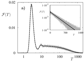
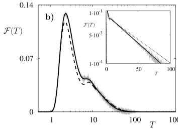
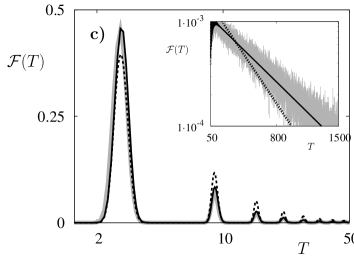
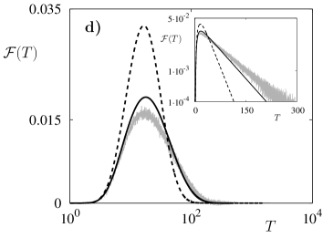
Fig. 1.–: FPT probability density for harmonic oscillator driven by Gaussian white noise. Simulation results are shown with a gray line, Hertz approximation with a black dashed line, and Stratonovich approximation with a black solid line. Note the logarithmic scale in $T$. The insets show the same curves on the logarithmic scale in ${\cal F}(T)$. The parameters are: $\omega_{0}=1,x_{0}=-1,v_{0}=0,x_{b}=1$, a) $\gamma=0.8,D=0.1,\tau_{rel}=2.5,T_{R}=343$, b) $\gamma=0.8,D=0.44,\tau_{rel}=2.5,T_{R}=15.6$, c) $\gamma=0.08,D=0.01,\tau_{rel}=25,T_{R}=343$, d) $\gamma=10.0,D=5.5,\omega_{0}/\gamma=0.1$

Let us first concentrate on the case (i) with white noise. In fig. 1 the FPT probability density obtained from simulations is compared with the Hertz and Stratonovich approximations (eq.(6) and eq.(9)). The probability to reach $x_{b}$ is higher in the maxima of the subthreshold oscillations. The initial phase of these oscillations is fixed by initial conditions. Thus on shorter time scales ${\cal F}(T)$ shows the multiple peaks following with the frequency of damped oscillations $\sqrt{\omega_{0}^{2}-\gamma^{2}/4}$. On long times $T\gg\tau_{rel}$ the quasiequilibrium establishes and FPT densities decay exponentially (see insets in fig. 1). The number of visible peaks depends on the relation between $\tau_{rel}$ and the period of oscillations and is given by the number of periods elapsing before the quasiequilibrium is achieved.

In fig.1(a) the parameters are chosen to be $\gamma=0.8,D=0.1$, corresponding to moderate friction and moderate noise intensity. For given parameter values $\tau_{rel}=2.5$ and $T_{R}=343$, so that $\tau_{rel}\ll T_{R}$, both Hertz and Stratonovich approximations hold and reproduce well the FPT density in the whole time domain.

In the case of moderate friction and stronger noise the upcrossings become more frequent and $T_{R}$ decreases. The FPT changes its form to practically monomodal with the only maximum and a small shoulder separating it from the tail. An example is given in fig.1(b) with $\gamma=0.8,D=0.44$ which correspond to $\tau_{rel}=2.5$ and $T_{R}=15.6$. The Stratonovich approximation complies very well with the simulations, while the Hertz approximation fails to reproduce the details of the distribution: It underestimates ${\cal F}(T)$ on short times, and shows slower exponential decay in the tail than the one observed in simulations (see the inset).

Finally, for small friction and low noise the upcrossings are rare, but the relaxation time is large. The FPT probability density exhibits multiple decaying peaks. In fig.1(c) $\gamma=0.08,D=0.01$ corresponding to $\tau_{rel}=25,T_{R}=343$. Again, the Stratonovich approximation performs well, while the Hertz approximation underestimates the first peak, overestimates all further peaks and decays in the tail faster than the simulated FPT density.

Fig. 1(d) corresponds to the overdamped regime ($\gamma>2\omega_{0}$) where the parameters are chosen to be $\gamma=10.0,D=5.5$ corresponding to $\omega_{0}/\gamma=0.1$. The condition $\tau_{rel}<T_{R}$ is always fulfilled in the overdamped case. However, with increasing friction the process $x(t)$ approaches the Markovian (diffusion) one, for which the pattern of upcrossings is very inhomogeneous. The successive crossings are strongly clustered [10]. The upcrossings within a cluster are not independent even if their mean density $n_{0}$ is low. This limits the accuracy of our approximations: The Stratonovich approximation starts to be inaccurate, and the Hertz approximation fails.

For $T$ large ${\cal F}(T)$ decays exponentially, ${\cal F}(T)\propto\exp(-\kappa T)$. The decrement of this decay is obtained from long time asymptotics: $\kappa T=\lim_{T\rightarrow\infty}S(T)$. Thus, in the Hertz approximation eq.(6) one gets $\kappa=(1/T)\lim_{T\rightarrow\infty}\int_{0}^{T}n_{1}(t)dt=n_{0}T/T=n_{0}$. The behaviour in the Stratonovich approximation eq.(9) is determined by $\lim_{t,t^{\prime}\rightarrow\infty}\int_{0}^{T}R(t,t^{\prime})n_{1}(t^{\prime})dt^{\prime}\approx n_{0}\tau_{cor}$ with $\tau_{cor}$ given by $\tau_{cor}=\lim\limits_{t\rightarrow\infty}\int_{0}^{\infty}R(t,t^{\prime})dt^{\prime}$. Note that $\tau_{cor}$ is not necessary positive. Inserting this expression into eq.(9) and expanding the logarithm up to the second term we get $\kappa=n_{0}(1+\frac{1}{2}n_{0}\tau_{cor})$ providing the second order correction to the previous expression. The value of $\tau_{cor}$ for the parameter set as in fig. 1(a) is $\tau_{cor}=-1\cdot 10^{-3}$, for parameters as in fig. 1(b) $\tau_{cor}=5.25$, and for parameters as in fig. 1(c) $\tau_{cor}=-396.7$. The long time asymptotics obtained with these $\tau_{cor}$ values reproduce fairly well the decay patterns found numerically.

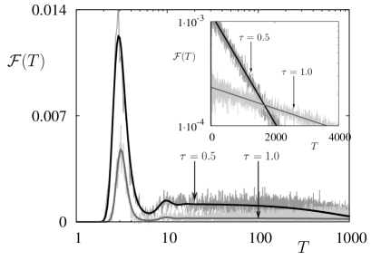
Fig. 2.–: Simulation results and the Hertz approximation for the FPT probability density for harmonic oscillator driven by Ornstein-Uhlenbeck noise with correlation times $\tau=0.5$ (upper curves) and $\tau=1.0$ (lower curves) and other parameters as in fig. 1(a). Note the logarithmic scale in $T$. The inset shows the same curves on the logarithmic scale in ${\cal F}(T)$.

Finally we consider our model (ii) having a higher dimension of its state space. In fig. 2 we show the simulated FPT probability density and the Hertz approximation for the system eq.(10) driven by the Ornstein-Uhlenbeck noise for two different values of the correlation time $\tau=0.5$ and $\tau=1.0$. In both cases the Hertz approximation is absolutely sufficient.

5 Conclusions

For the case of moderate friction and moderate noise intensity the Hertz approximation is absolutely sufficient. The Stratonovich approximation performs evenly well and does not lose accuracy for high noise intensity. The validity region of approximations covers all different types of subthreshold dynamics, and reproduces all qualitative different structures of the FPT PDF: from monomodal through bimodal to multimodal densities with decaying peaks. The approximations work for the systems of whatever dimension and are especially effective for the processes with narrow spectral density, exactly when Markovian approximations fail.

We acknowledge financial support from the DFG by Graduierten-Kolleg 268 and the Bernstein Center for Computational Neuroscience, Berlin and Sfb555.

References

- [1] E. Schrödinger, Physik. Z. 16, 289 (1915).
- [2] P. Hänggi, P. Talkner, and M. Brokovec, Rev. Mod. Phys. 62, 251 (1990).
- [3] A. Longtin, A. Bulsara, and F. Moss, Phys. Rev. Lett. 67, 656 (1991).
- [4] H.C. Tuckwell, Introduction to Theoretical Neurobiology, vol. 2 (Cambridge University Press, Cambridge UK, 1988).
- [5] S. Redner, A Guide to First-Passage Processes (Cambridge University Press, Cambridge UK, 2001).
- [6] H. Risken, The Fokker-Planck Equation (Springer, Berlin, 1996).
- [7] N. G. van Kampen, Stochastic Processes in Physics and Chemistry (North-Holland, Amsterdam 1992).
- [8] V.I. Tikhonov, M.A. Mironov, Markovian Processes (Sov. Radio, Moscow, 1977).
- [9] G.L. Gerstein, and B. Mandelbrot, Biophys. J. 4, 41 (1964).
- [10] R.L. Stratonovich, Topics in the Theory of Random Noise, vol. 2 (Gordon and Breach, New York, 1967).
- [11] B. Lindner, Phys. Rev. E 69, 022901 (2004).
- [12] D. Sigeti and W. Horsthemke, J. Stat. Phys. 54, 1217 (1989).
- [13] S. Liepold, J.A. Freund, L. Schimansky-Geier, A. Neiman, and D. Russell, Journ. Theor. Biophys., in print.
- [14] B. Lindner, J. García-Ojalvo, A. Neiman, and L. Schimansky-Geier, Phys. Reports 392, 321 (2004).
- [15] I. Erchova, G. Kreck, U. Heinemann, and A.V.M. Herz, J. Physiol. 560, 89 (2004).
- [16] T. Verechtchaguina, L. Schimansky-Geier, and I.M. Sokolov, Phys. Rev. E 70, 031916 (2004).
- [17] E.M. Izhikevich, Neural Netw. 14, 883 (2001).
- [18] A.M. Lacasta, F. Sagues, and J.M. Sancho, Phys. Rev. E 66, 045105(R) (2002).
- [19] N. Brunel, V. Hakim and M.J.E. Richardson, Phys. Rev. E, 67, 051916 (2003).
- [20] S.M. Soskin, V.I. Sheka, T.L. Linnik, and R. Mannella, Phys. Rev. Lett., 86, 1665 (2001).
- [21] S.O. Rice, Bell System Tech. J. 24, 51 (1945).
- [22] A.J.F. Siegert, Phys. Rev. 81, 617 (1951).
- [23] Ya.A. Fomin, Excursions Theory of Stochastic Processes (Svyaz, Moscow, 1980).
- [24] P. Hertz, Math. Ann. 67, 387 (1909).
- [25] P. Jung, Phys. Rev. E 50, 2513 (1994).