Exact results for the D interacting mixed Bose-Fermi gas
Abstract
The exact solution of the D interacting mixed Bose-Fermi gas is used to calculate ground-state properties both for finite systems and in the thermodynamic limit. The quasimomentum distribution, ground-state energy and generalized velocities are obtained as functions of the interaction strength both for polarized and non-polarized fermions. We do not observe any demixing instability of the system for repulsive interactions.
pacs:
03.75.Ss, 05.30.Fk, 67.60.-g,71.10.PmThe cooling and trapping of quantum Fermi gases of ultracold atoms poses a number of additional challenges to those faced for bosons BEC . A key point is that no more than one identical fermion can occupy a single state due to the Pauli exclusion principle. However, a mixed gas of fermions and bosons provides an effective means of cooling single-component fermions by thermal collisions with evaporatively cooled bosons Fermi-1 ; Fermi-2 ; Fermi-3 ; Fermi-4 , providing an avenue for investigating many-body quantum effects in degenerate Fermi gases. Another development is the use of Feshbach resonance, in which the energy of a bound state of two colliding atoms is magnetic field tuned to vary the scattering strength from to , allowing the investigation of the crossover from BCS superfluidity to Bose-Einstein condensation BEC-F1 ; BEC-F2 ; BEC-F3 . These achievements in realizing quantum Fermi gases of ultracold atoms may also provide insights into other areas of physics, such as ultracold superstrings superstring .
Particular theoretical and experimental interest has been paid to the Fermi gas confined in 1D geometry Fermi-1D1 ; Fermi-1D2 ; BEC-BCS1 ; BEC-BCS2 ; BEC-BCS3 . Recent attention has turned to the 1D model of mixed bosons and polarized fermions mix-1 ; mix-2 ; mix-3 ; mix-4 , revealing quantum effects such as interaction-driven phase separation phase-s1 ; mix-3 ; mix-4 , bright solitons in degenerate Bose-Fermi mixtures kar04 and Luttinger liquid behaviour mix-1 ; mix-2 . In this model, only -wave scattering for boson-boson and boson-fermion interactions is considered, with the boson-fermion collisions minimizing the Pauli-blocking effect in momentum space.
The theoretical studies of the mixed Bose-Fermi gas have focused on the case of bosons and single-component fermions mix-1 ; mix-2 ; mix-3 ; mix-4 . Our aim here is to investigate the D model of a Bose-Fermi mixture on a line of length with periodic boundary conditions, with Hamiltonian , where among the particles there are fermions and bosons. The pairwise -interaction has strength . The crucial observation from a theoretical point of view is that if all particles have equal masses and if the interaction strength between all particles is the same, the above model is exactly solvable by Bethe Ansatz (BA) L-Y . Although this restricts the applicability of the model, experiments with isotopes of atoms are expected to meet the BA conditions mix-4 . Then , where is the inverse 1D scattering length of the confined particles. For convenience of notation, the energy is measured in units of , such that
| (1) |
The model contains two special limiting cases: (i) the D interacting Fermi gas with arbitrary polarization Yang-Gaudin ; Takahashi ; Wadati ; BBGN , and (ii) the D interacting Bose gas LL63 . The mixed model was recently discussed for the case of single component (fully polarized) fermions mix-4 . Here we consider the more general case of two-component fermions with arbitrary polarization. We present analytical and numerical results for the ground state energy, quasimomentum density profile, and the spin and charge velocities. In the weak coupling limit, these quantities reveal the typical signatures of pure quantum gases with an additional weak interaction due to the mixture. In the other extreme, that is for strong repulsive interactions, the ground state properties resemble those of a single-component non-interacting Fermi gas.
The BA equations (BE), determining the quantum numbers of the -particle system, are given by L-Y
| (2) | |||||
| (3) | |||||
| (4) |
where and , , . Without loss of generality, we take . Here the set of many quantum numbers is divided into three subsets: , , . It turns out that the energy eigenvalues are given by the members of the first set alone, namely .
We begin with a finite system, for which the Bethe roots are found analytically in the weak coupling limit, thereby yielding the ground state energy. The second step is to carry out the thermodynamic limit (TL). In this limit, the Bethe roots are distributed smoothly over a certain interval of the real axis, giving rise to continuous densities. Integral equations for these densities have been obtained previously L-Y . On the one hand, these equations allow a comparison between the analytical results for weak coupling and finite systems with the weak coupling expansion in the TL. On the other hand, generalized velocities can be calculated within this framework. In the weak coupling limit, these reduce to the spin and charge velocities of a pure Fermi gas and the charge velocity of a pure bosonic system.
In considering the ground state for weak interaction, it is convenient to distinguish between unpaired (), paired () and bosonic () quasimomenta note1 . Expanding Eqs. (2)-(4) to , one obtains , ; and . Here if odd and if even. The deviations from are linear in , with
| (5) | |||||
| (6) |
Here denotes the quasimomenta in the free particle limit as given above. The sums in (5), (6) over paired momenta count each pair only once. The bosonic momenta collapse at the origin for . Their -dependence is given by
| (7) |
According to (7), the are the roots of Hermite polynomials of degree gau71 ; BGM .
From the above equations we obtain the ground state energy, , to leading order in . The energy of the free particles, , is given by the corresponding expression for a free Fermi gas with fermions BBGN . The first correction in is , where () is the linear order in for a pure Bose (Fermi) gas of bosons BGM ( fermions BBGN ). The last term is due to the interactions between bosons and fermions. Thus
| (8) | |||||
This expression is valid for both weak repulsive and attractive interaction. Especially, the TL is well defined in the weakly attractive case, as opposed to the strongly attractive case Takahashi . Let us now carry out the TL, i.e., where the densities are held constant, with . In this limit, Eqs. (5) and (6) give the distribution of quasimomenta per unit length,
| (9) | |||||
| (10) | |||||
| (11) |
where , , .
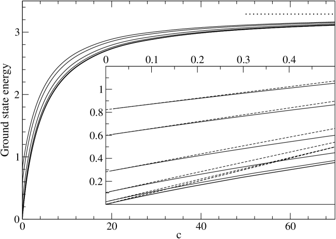
The quasimomentum distribution function of the bosonic momenta (11) for is given by the semi-circular law behaviour as for a pure bosonic system LL63 ; gau71 ; BGM . For , the in (7) are imaginary, so that (11) with imaginary yields the dark-soliton like distributions of the bosonic quasimomenta on the imaginary axis. These encode the binding energy of the bosons, a quantity potentially accessible by experiments. In the distribution of the fermionic quasimomenta, divergences occur near the cutoffs. The quasimomentum distribution functions calculated from the BE (2)-(4) are compared with the approximations (9)-(11) in Fig. 1.
In order to study the effect of arbitrary interaction in the TL, we use the linear integral equations derived by Lai and Yang L-Y which determine the densities of the quasimomenta. In the following, we restrict ourselves to two limiting cases, namely and . In the latter case, the fermions do not interact among themselves due to the Pauli principle, so that the interaction potential in (1) is only effective between fermions and bosons. The ground-state energy for this case has been calculated recently mix-4 . In the other limiting case, , all the fermions interact with each other and with the bosons. Fig. 2 shows the ground-state energy per unit length for different densities and obtained from numerical solution of the integral equations. Also shown is a comparison between the analytic result (8) and the TL.
Up to this point, we have focussed on the density of the quasimomenta . In an analogous fashion, one may introduce densities , of the roots . Using the dressed energy formalism Takahashi , one can calculate the corresponding dressed energies , which are the energies necessary to add or remove a root to or from the seas of . The dressed energies give rise to generalized velocities, which determine the asymptotics of correlation functions frahm . In the case of pure bosons, there is only one species of BE numbers, associated with one dressed energy function, yielding the charge (or sound) velocity LL63 ; Takahashi . For pure fermions, the two sets of BE numbers are linked with the charge and spin velocities . As has been proven by Haldane hal81a , these velocities coincide with those calculated in the harmonic-fluid (or bosonization) approach hal81b .
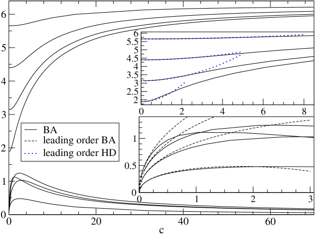
The situation is less clear for the mixture of bosons and fermions. In the BA approach, this corresponds to two seas of BE numbers , and correspondingly two dressed energies and two velocities, which we call . For we have and . The dependence of on for different values of is shown in Fig. 3. The lowest -order of is obtained from the Bethe-Ansatz as , which is the velocity of a non-interacting Bose gas for small LL63 .
We now compare our results to those of the hydrodynamic (HD) approach mix-1 . In this framework, the pure gases correspond to harmonic oscillators, such that the coupling between them leads to new normal modes , with . In the weak interaction limit, , . For the sake of comparison, the latter result is also shown in Fig. 4. In the strongly repulsive limit, a demixing instability is predicted from the HD mix-1 and mean-field approaches mix-3 . We do not observe any instability for repulsive interaction for the integrable model, in agreement with L-Y ; mix-4 . The reason for the discrepancy is that to our present understanding, the HD approach for the mixture, especially the calculation of normal modes, is a low-energy theory. That is, it is expected to yield reliable results for small interaction strengths . Investigation of within the BA approach in the strongly repulsive limit yields
where .
It remains a very interesting question for future research if the normal modes of the field theory coincide with the generalized velocities from the BA for mixed Bose-Fermi systems. Furthermore, it should be carefully investigated whether or not the HD approach is applicable in the strongly interacting regime.
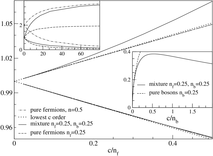
The generalized velocities can also be computed from the BA for interacting fermions (). In this case, the three dressed energies give rise to three velocities, which we call and . As shown in Fig. 4, we observe that in the weak interaction limit, , which corresponds to the charge and spin velocities of a pure fermionic system BEC-BCS1 . In the strong interaction limit, , whereas . This again indicates the fermionic nature of the system in the strongly interacting limit.
In conclusion, we have investigated ground state properties of the 1D interacting Bose-Fermi model from its exact BA solution. We obtained results for the distribution of quasimomenta and the ground state energy both for weak attractive and repulsive interactions. We computed the generalized velocities and compared them to the normal modes obtained from the HD approach. In contrast with other approaches mix-1 ; mix-3 ; mori , we do not observe any instability or demixing in the system.
Acknowledgements. This work has been supported by the Australian Research Council and the German Science Foundation under grant number BO/2538.
References
- (1) M. H. Anderson, J. R. Ensher, M. R. Matthews, C. E. Wieman and E. A. Cornell, Science 269 (1995) 98; K. B. Davis et al, Phys. Rev. Lett. 75 (1995) 3969.
- (2) A. G. Truscott, K. E. Strecker, W. I. McAlexander, G. B. Partridge, R. G. Hulet, Science 291 (2001) 2570.
- (3) Z. Hadzibabic et al, Phys. Rev. Lett. 88 (2002) 160401.
- (4) Z. Hadzibabic et al, Phys. Rev. Lett. 91 (2003) 160401.
- (5) C. Silber et al, cond-mat/0506217.
- (6) S. Jochim et al, Science 302 (2003) 2101; C. Chin et al, Science 305 (2004) 1128.
- (7) M. W. Zwierlein et al, Phys. Rev. Lett. 91 (2003) 250401.
- (8) C. A. Regal, M. Greiner and D. S. Jin, Phys. Rev. Lett. 92 (2004) 040403.
- (9) M. Snoek, M Haque, S. Vandoren and H.T.C. Stoof, cond-mat/0505055.
- (10) H. Moritz, T. Stöferle, K. Günter, M. Köhl and T. Esslinger, Phys. Rev. Lett. 94 (2005) 210401.
- (11) A. Recati, J. N.Fuchs and W. Zwerger, Phys. Rev. A. 71 (2005) 033630.
- (12) J. N. Fuchs, A. Recati and W. Zwerger, Phys. Rev. Lett. 93 (2004) 090408.
- (13) G. E. Astrakharchik, D. Blume, S. Giorgini and L.P. Pitaevskii, Phys. Rev. Lett. 93 (2004) 050402.
- (14) I. V. Tokatly, Phys. Rev. Lett. 93 (2004) 090405.
- (15) M. A. Cazalilla and A. F. Ho, Phys. Rev. Lett. 91 (2003) 150403.
- (16) L. Mathey et al, Phys. Rev. Lett. 93 (2004) 120404.
- (17) K. K. Das, Phys. Rev. Lett. 90 (2003) 170403.
- (18) A. Imambekov and E. Demler, cond-mat/0505632.
- (19) K. Mølmer, Phys. Rev. Lett. 80 (1998) 1804.
- (20) T. Karpiuk et al., Phys. Rev. Lett. 93 (2004) 100401
- (21) C.K. Lai and C.N. Yang, Phys. Rev. A 3 (1971) 393.
- (22) M. Gaudin, Phys. Lett. A 24 (1967) 1312; C.N. Yang, Phys. Rev. Lett. 19 (1967) 1312.
- (23) M. Takahashi, Thermodynamics of One-Dimensional Solvable Models (Cambridge, Cambridge University Press, 1999).
- (24) T. Iida and M. Wadati, J. Phys. Soc. Jpn. 74 (2005) 1724.
- (25) M. T. Batchelor, M. Bortz, X.W. Guan and N. Oelkers, cond-mat/0506264.
- (26) E. H. Lieb and W. Liniger, Phys. Rev. 130 (1963) 1605; E. H. Lieb, Phys. Rev. 130 (1963) 1616.
- (27) Since the substitution of two fermions into bosons is equivalent to increasing to , there are momenta .
- (28) M. Gaudin, Phys. Rev. A 4 (1971) 386.
- (29) M.T. Batchelor, X.W. Guan and J.B. McGuire, J. Phys. A 37 (2004) L497.
- (30) H. Frahm and G. Palacios, cond-mat/0507368.
- (31) F. D. M. Haldane, Phys. Lett. 81A (1981) 153.
- (32) F. D. M. Haldane, Phys. Rev. Lett. 47 (1981) 1840.
- (33) Y. Takeuchi and H. Mori, cond-mat/0508247.