Quantum Transport from the Perspective of Quantum Open Systems

Abstract

By viewing the non-equilibrium transport setup as a quantum open system, we propose a reduced-density-matrix based quantum transport formalism. At the level of self-consistent Born approximation, it can precisely account for the correlation between tunneling and the system internal many-body interaction, leading to certain novel behavior such as the non-equilibrium Kondo effect. It also opens a new way to construct time-dependent density functional theory for transport through large-scale complex systems.

Conventionally, quantum transport and quantum dissipation are treated with different approaches. For instance, the former (in mesoscopic context) is usually described by the Landauer-Büttiker theory and the non-equilibrium Green’s function (nGF) approach Dat95 ; Hau96 , whereas the latter by the reduced density matrix equation Gar00 . Nevertheless, both are quantum open systems, with either the non-equilibrium electron reservoirs (electrodes) or the dissipative thermal bath as their environments, as schematically shown in Fig. 1. It is thus of great interest to develop a unified language to bridge them.

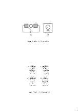
Figure 1: A unified picture for (A) quantum transport and (B) quantum dissipative open system, where the transport system is regarded as the “system of interest”, and the electrodes as “environmental baths”.

This motivation can be historically dated back to the phenomenological rate equation and quantum Bloch equation approaches to transport Gla88 ; Gur96 . There, either implicitly or explicitly, the electrodes are viewed as dissipative reservoirs. Along this line and based on our work in quantum measurement of solid-state qubit Li04a ; Li04b , we developed recently a quantum master equation approach to quantum transport Li04c . The reduced dynamics involved there was originally constructed under the cumulant second-order expansion (Born approximation). In this letter, we re-formalize it in the spirit of self-consistent Born approximation (SCBA), in order to make the formalism not only convenient but also accurate enough in practice. Moreover, by reducing the many-particle density matrix formalism to single-particle one, we will also construct an efficient approach for large-scale (e.g. molecular) system applications.

The typical transport setup, see Fig. 1(A), can be described by

$$H = H_{S}(a_{\mu}^{\dagger},a_{\mu})+\sum_{\alpha=L,R}\sum_{\mu k}\epsilon_{\alpha\mu k}d^{\dagger}_{\alpha\mu k}d_{\alpha\mu k}$$ (1)

$$+\sum_{\alpha=L,R}\sum_{\mu k}(t_{\alpha\mu k}a^{\dagger}_{\mu}d_{\alpha\mu k}+\rm{H.c.}).$$

$H_{S}$ is the system Hamiltonian, which can be rather general (e.g. including many-body interaction). $a^{\dagger}_{\mu}$ ($a_{\mu}$) is the creation (annihilation) operator of electron in state labelled by “$\mu$”, which labels both the multi-orbital and distinct spin states of the transport system. The second and third terms describe, respectively, the two (left and right) electrodes and the tunneling between the electrodes and the system.

To contact with the quantum dissipation theory for quantum open systems, let us introduce the reservoir operators $F_{\mu}=\sum_{\alpha k}t_{\alpha\mu k}d_{\alpha\mu k}\equiv f_{L\mu}+f_{R\mu}$. Accordingly, the tunneling Hamiltonian $H^{\prime}$ reads $H^{\prime}=\sum_{\mu}\left(a^{\dagger}_{\mu}F_{\mu}+\rm{H.c.}\right)$. Treating $H^{\prime}$ perturbatively up to the cumulant second-order expansion, it yields Yan98

$$\dot{\rho}(t)=-i{\cal L}\rho(t)-\int_{0}^{t}d\tau\langle{\cal L}^{\prime}(t){\cal G}(t,\tau){\cal L}^{\prime}(\tau){\cal G}^{\dagger}(t,\tau)\rangle\rho(t).$$ (2)

The reduced density matrix is defined as $\rho(t)=\rm{Tr}_{B}[\rho_{T}(t)]$, by tracing out the reservoir degrees of freedom from the total system-plus-reservoirs density matrix. The Liouvillian superoperators are defined as ${\cal L}(\cdots)\equiv[H_{S},(\cdots)]$, ${\cal L^{\prime}}(\cdots)\equiv[H^{\prime},(\cdots)]$, and ${\cal G}(t,\tau)(\cdots)\equiv G(t,\tau)(\cdots)G^{\dagger}(t,\tau)$ with $G(t,\tau)$ the usual propagator (Green’s function) associated with the system Hamiltonian $H_{S}$.

The integral kernel in Eq. (2), which is in the so-called partial ordering prescription (POP) (or time-local) form Yan98 , describes the second-order tunneling self-energy. At the second-order level, one may replace $\rho(t)$ in the last term of Eq. (2) with ${\cal G}(t,\tau)\rho(\tau)$, leading the tunneling integral kernel to $\langle{\cal L}^{\prime}(t){\cal G}(t,\tau){\cal L}^{\prime}(\tau)\rangle\rho(\tau)$, being in the chronological ordering prescription (COP) (or memory) form Yan98 . The corresponding four terms in the conventional Hilbert space Li04b ; Li04c , depicted on the real-time Keldysh contour in Fig. 2, provide a clear diagrammatic interpretation for the second-order tunneling self-energy process.

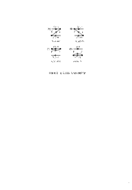
Figure 2: Diagrammatic illustration for the second-order tunneling self-energy processes, on the Keldysh contour. The upper and lower horizontal lines describe the forward and backward propagation of the transport system, which is treated exactly in terms of the system Green’s function $G(t,\tau)$. The dashed line stands for the tunneling between the system and electrodes.

Explicitly tracing out the states of electrodes, Eq. (2) gives rise to

$$\dot{\rho} = -i{\cal L}\rho-\sum_{\mu}\left\{[a_{\mu}^{\dagger},A_{\mu}^{(-)}\rho-\rho A_{\mu}^{(+)}]+\rm{H.c.}\right\}.$$ (3)

For time-independent system Hamiltonian, $A^{(\pm)}_{\mu}=\sum_{\alpha=L,R}A^{(\pm)}_{\alpha\mu}=\sum_{\alpha\nu}\int_{-\infty}^{\infty}\!\!dt\,C^{(\pm)}_{\alpha\mu\nu}(\mp t)[i{\tilde{a}}_{\nu}(t)]$, with $C^{(+)}_{\alpha\mu\nu}(t)\equiv\langle f^{\dagger}_{\alpha\mu}(t)f_{\alpha\nu}(0)\rangle$, $C^{(-)}_{\alpha\mu\nu}(t)\equiv\langle f_{\alpha\mu}(t)f_{\alpha\nu}^{\dagger}(0)\rangle$, and ${\tilde{a}}_{\nu}(t)=-i\Theta(t){\cal G}(t,0)a_{\nu}\equiv\Pi^{(0)}(t,0)a_{\nu}$. Note that the step function $\Theta(t)$ extends the lower bound of the time integral from $0$ to $-\infty$, whereas the extension of the upper bound from $t$ to $\infty$ results from the consideration of Markovian approximation.

For time-dependent system Hamiltonian, the time-translational invariance breaks down, we thus define ${\tilde{a}}_{\nu}(t,t^{\prime})=-i\Theta(t-t^{\prime}){\cal G}(t,t^{\prime})a_{\nu}$. The backward evolution of $\tilde{a}_{\nu}(t,t^{\prime})$ with respect to $t^{\prime}$, starting from $t^{\prime}=t$, can be carried out via $\partial_{t^{\prime}}a_{\nu}(t,t^{\prime})=i\delta(t-t^{\prime})a_{\nu}+i[H_{S}(t^{\prime}),a_{\nu}(t,t^{\prime})]$. Thus, the time integral in $A_{\mu}^{(\pm)}$, which becomes now the type of $\sim\int^{t}_{0}dt^{\prime}C^{(\pm)}_{\alpha\mu\nu}(t-t^{\prime}){\tilde{a}}_{\nu}(t,t^{\prime})$, can be calculated accordingly. Inserting the obtained $A_{\mu}^{(\pm)}$ into Eq. (3), the time-dependent phenomena associated with either quantum dissipative dynamics or transport current can be easily treated. For clarity, we hereafter assume the system Hamiltonian to be time-independent, unless further specification.

Now we consider the possibility to go beyond the second-order self-energy process diagrammatically shown in Fig. 1. An efficient scheme follows the idea of the well-known self-consistent Born approximation (SCBA), i.e., the free propagator defined above, $\Pi^{(0)}(t)\equiv-i\Theta(t){\cal G}(t,0)$, is replaced by an effective propagator $\Pi(t)$. The latter is obtained formally via the Dyson equation note-2

$$\dot{\Pi}(t)=-i\delta(t)-i{\cal L}\Pi(t)-i\int^{t}_{-\infty}dt^{\prime}\Sigma(t-t^{\prime})\Pi(t^{\prime}),$$ (4)

or $\Pi(\omega)=[\omega-{\cal L}-\Sigma(\omega)]^{-1}$ in frequency domain, with $\Sigma$ being the irreducible self-energy defined again by Fig. 2. Accordingly, $\tilde{a}_{\nu}(t)=\Pi(t)a_{\nu}$, and

$$A^{(\pm)}_{\mu}=\sum_{\alpha\nu}\int\frac{d\omega}{2\pi}C^{(\pm)}_{\alpha\mu\nu}(\pm\omega)[i\Pi(\omega)a_{\nu}].$$ (5)

Equations (3)–(5) constitute the basic ingredients of the proposed SCBA scheme. This type of self-consistently partial summation correction has included an infinite number of higher order tunneling processes into the reduced system dynamics. The resulting non-trivial effect on quantum transport will be demonstrated soon.

So far, the trace is performed over all the electrode states, and the resulting Eq. (3) is a unconditional master equation for the system reduced dynamics. To characterize the transport problem, we should keep track of the record of electron numbers entering the right reservoir (electrode). Following Refs. Li04b, and Li04c, , one can obtain a conditional master equation for the reduced system density matrix, $\rho^{(n)}(t)$, under the condition that $n$ electrons have arrived at the right electrode until time $t$. On the basis of $\rho^{(n)}(t)$, one is readily able to compute various transport properties, such as the transport current, the probability distribution function $P(n,t)\equiv\rm{Tr}[\rho^{(n)}(t)]$, and the noise spectrum Li04b . For transport current, it can be carried out via $I(t)=e\sum_{n}n\rm{Tr}[\dot{\rho}^{(n)}(t)$, giving rise to

$$I(t)=e\sum_{\mu}\rm{Tr}\left[\left(a^{\dagger}_{\mu}A^{(-)}_{R\mu}-A^{(+)}_{R\mu}a^{\dagger}_{\mu}\right)\rho(t)+\rm{H.c.}\right].$$ (6)

Compared to other transport formalisms, Eqs. (3)-(6) provide a convenient framework for quantum transport.

As an illustrative application, we consider the non-trivial problem of quantum transport through strongly interacting quantum dot, under the well-known Anderson impurity model Hamiltonian: $H_{S}=\sum_{\mu}(\epsilon_{0}a_{\mu}^{\dagger}a_{\mu}+\frac{U}{2}n_{\mu}n_{\bar{\mu}})$. Here the index $\mu$ labels the spin up (“$\uparrow$”) and spin down (“$\downarrow$”) states, and $\bar{\mu}$ stands for the opposite spin orientation. The electron number operator $n_{\mu}=a^{\dagger}_{\mu}a_{\mu}$, and the Hubbard term $Un_{\uparrow}n_{\downarrow}$ describe the charging effect. Apparently, the reservoir correlation function is diagonal with respect to the spin indices, i.e., $C^{(\pm)}_{\alpha\mu\nu}(t)=\delta_{\mu\nu}C^{(\pm)}_{\alpha\mu\mu}(t)$, and $C_{\alpha\mu\mu}^{(\pm)}(t)=\sum_{k}|t_{\alpha\mu k}|^{2}e^{\pm i\epsilon_{k}(t)}n^{(\pm)}_{\alpha}(\epsilon_{k})$. Here $n^{(+)}_{\alpha}(\epsilon_{k})=n_{\alpha}(\epsilon_{k})$ is the Fermi distribution function, and $n^{(-)}_{\alpha}(\epsilon_{k})=1-n_{\alpha}(\epsilon_{k})$. Accordingly, we have $A^{(\pm)}_{\alpha\mu}=\Gamma_{\alpha\mu}\int\frac{d\epsilon}{2\pi}n_{\alpha}^{(\pm)}(\epsilon)[i\Pi(\epsilon)]a_{\mu}$, where, under the wide-band approximation, we have introduced $\Gamma_{\alpha\mu}=2\pi g_{\alpha}|t_{\alpha\mu k}|^{2}$, and assumed it energy independent. From Eqs. (6) and (3), the stationary current is obtained as

$$I = \frac{e\Gamma_{L}\Gamma_{R}}{\Gamma_{L}+\Gamma_{R}}\int\frac{d\epsilon}{2\pi}{\rm Im}[\Pi(\epsilon)][n_{L}(\epsilon)-n_{R}(\epsilon)].$$ (7)

For the single level system under study, the propagator in energy space simply reads $\Pi(\epsilon)=[\epsilon-\epsilon_{0}-\Sigma(\epsilon)]^{-1}$.

Within the SCBA scheme, the self-energy $\Sigma$ can be explicitly carried out via Fig. 2. However, in the case of strong Coulomb repulsion, the dot can be occupied at most by one electron. As a result, it can be easily proven that only Fig. 2(C) and (D) contribute to the self-energy. Physically, replacing the bare system propagator with the effective propagator corresponds to including the infinitely multiple forward and backward tunnelings between the system and the same electrode. This is in fact a tunneling-induced quantum fluctuation, which would lead to the level broadening and the non-trivial interference between tunneling and system internal interaction. Explicitly, in large-$U$ limit, the real and imaginary parts of the self-energy read ${\rm Re}\Sigma(\epsilon)=(m-1)\sum_{\alpha=L,R}\frac{\Gamma_{\alpha\mu}}{2\pi}\Big{[}\ln\Big{(}\frac{\beta U}{2\pi}\Big{)}-{\rm Re}\psi\Big{(}\frac{1}{2}+i\frac{\beta}{2\pi}(\epsilon-\mu_{\alpha})\Big{)}\Big{]}$ and ${\rm Im}\Sigma(\epsilon)=-\sum_{\alpha=L,R}\frac{\Gamma_{\alpha\mu}}{2}\Big{[}1+(m-1)n_{\alpha}(\epsilon)\Big{]}$, respectively Sch94 ; Kon96 . Here $\beta\equiv 1/(k_{B}T)$ is the inverse temperature, $\mu_{\alpha}$ the chemical potential of the electrode, $\psi$ the digamma function, and $m$ denotes the spin degeneracy. (i) For $m=1$, i.e. neglecting the spin degree of freedom, ${\rm Im}\Pi(\epsilon)$ gives the well-known Breit-Wigner formula, which appropriately includes the level broadening effect. (ii) For $m\geq 2$ (e.g., $m=2$ for spin $1/2$), the above self-energy correction would result in rich behaviors, depending on the relative values of the parameters such as the temperature and the position of $\epsilon_{0}$ with respect to the Fermi levels. Detailed discussions, in particular the non-equilibrium Kondo effect, are referred to literature, e.g. Refs. Kon96, -Mei93, .

Application to Large Scale Systems.— By far, the transport-related density matrix formalism has been constructed in many-particle Hilbert space, which may restrict its direct application only in small systems. For large-scale systems in the absence of many-electron interaction, we first recast the formalism to a very simple version in terms of the reduced single-particle density matrix (RSPDM), $\sigma_{\mu\nu}(t)\equiv\rm{Tr}[a^{\dagger}_{\nu}a_{\mu}\rho(t)]$, which greatly reduces the dimension of Hilbert space, thus saves computing expense. To account for the electron-electron interaction, we then propose an efficient time-dependent density functional theory (TDDFT) scheme. Note that it is quite natural to combine the TDDFT technique with the present RSPDM formalism, since the former self-consistently amounts to the many-body interaction but still keeps the single-particle picture note-5 .

(i) Time Independent System Hamiltonian: For simplicity, we first proceed our derivation in the single-particle eigenstate basis, which is denoted as $\{|\mu\rangle,|\nu\rangle,\cdots\}$. In this representation, $A_{\alpha\mu}^{(\pm)}=\sum_{\nu}C^{(\pm)}_{\alpha\mu\nu}(\mp\epsilon_{\nu})a_{\nu}$, and the equation of motion for the RSPDM can be readily obtained by applying Eq. (3) directly for $\sigma_{\mu\nu}(t)=\rm{Tr}[a^{\dagger}_{\nu}a_{\mu}\rho(t)]$. We have note-4 ; Yok04

$$\dot{\sigma}=-i[h,\sigma]-\frac{1}{2}\left\{\left[C^{(-)}\sigma-C^{(+)}\bar{\sigma}\right]+\rm{H.c.}\right\}.$$ (8)

Here, $h$ is the single-particle Hamiltonian or the Fock matrix within the TDDFT framework which will be identified soon. $\bar{\sigma}\equiv 1-\sigma$ denotes the “hole” density matrix. The involving matrix products are defined as usual; e.g., $[C^{(-)}\sigma]_{\mu\nu}\equiv\sum_{\alpha=L,R}\sum_{\nu^{\prime}}C^{(-)}_{\alpha\mu\nu^{\prime}}(\epsilon_{\nu^{\prime}})\sigma_{\nu^{\prime}\nu}$. Straightforwardly, the current can be expressed in terms of the RSPDM as

$$I(t)=e\rm{Re}\left\{\rm{Tr}\left[C^{(-)}_{R}\sigma(t)-C^{(+)}_{R}\bar{\sigma}(t)\right]\right\}.$$ (9)

In arbitrary state basis, derivation is the same as above. The difference lies only at the expression of $A_{\alpha\mu}^{(\pm)}$, which in a non-eigenstate representation is given formally as $A_{\alpha\mu}^{(\pm)}\equiv\sum_{\nu}\tilde{C}^{(\pm)}_{\alpha\mu\nu}a_{\nu}=\sum_{\nu\nu^{\prime},m}C^{(\pm)}_{\alpha\mu\nu^{\prime}}(\mp\epsilon_{m})D^{-1}_{\nu^{\prime}m}D_{m\nu}a_{\nu}$. Here $\epsilon_{m}$ is the eigen-energy of eigenstate $|m\rangle$, and $D$ is the transformation matrix from the non-eigestate representation to the eigenstate one. Obviously, with this identification, the resultant master equation and current formula are the same as Eqs. (8) and (9), only replacing the matrices $C^{(\pm)}$ by $\tilde{C}^{(\pm)}$.

As an illustrative application of Eqs. (8) and (9), we consider the simple non-interacting multi-level model studied in Ref. Li04c, . In the non-equilibrium stationary state, $\sigma(t\rightarrow\infty)$ is diagonal in the eigenstate basis, thus $[h,\sigma]=0$. As a consequence, the stationary state solution is determined by $C^{(-)}_{\mu\mu}(\epsilon_{\mu})\sigma_{\mu\mu}=C^{(+)}_{\mu\mu}(-\epsilon_{\mu})(1-\sigma_{\mu\mu})$, leading to the well-known result Li04c , $\sigma_{\mu\mu}=[\Gamma_{L}(\epsilon_{\mu})n_{L}(\epsilon_{\mu})+n_{R}(\epsilon_{\mu})\Gamma_{R}(\epsilon_{\mu})]/[\Gamma_{L}(\epsilon_{\mu})+\Gamma_{R}(\epsilon_{\mu})]$. In particular, in the special case of equilibrium, $\sigma_{\mu\mu}$ reduces to the Fermi-Dirac function. Substituting $\sigma_{\mu\mu}$ into Eq. (9), the well-known resonant tunnel current is obtained.

(ii) Time Dependent System Hamiltonian: In this case, the RSPDM can be introduced in a similar manner. Consider, for example, ${\rm Tr}[a^{\dagger}_{\mu}A^{(-)}_{\nu}\rho(t)]=\sum_{\alpha\nu^{\prime}}\int^{t}_{0}dt^{\prime}C^{(-)}_{\alpha\nu\nu^{\prime}}(t,t^{\prime})\sigma_{\nu^{\prime}\mu}(t^{\prime},t)\equiv[C^{(-)}\sigma]_{\nu\mu}$. Here, $\sigma_{\nu^{\prime}\mu}(t^{\prime},t)\equiv{\rm Tr}\{a^{\dagger}_{\mu}[{\cal G}(t,t^{\prime})a_{\nu^{\prime}}]\rho(t)\}$, which can be solved via $\partial_{t^{\prime}}\sigma_{\nu^{\prime}\mu}(t^{\prime},t)=-i[h(t^{\prime})\sigma(t^{\prime},t)]_{\nu^{\prime}\mu}$, with the initial condition $\sigma_{\nu^{\prime}\mu}(t,t)={\rm Tr}[a^{\dagger}_{\mu}a_{\nu^{\prime}}\rho(t)]$. Similarly, we have ${\rm Tr}[A^{(+)}_{\nu}a^{\dagger}_{\mu}\rho(t)]=\sum_{\alpha\nu^{\prime}}\int^{t}_{0}dt^{\prime}C^{(+)}_{\alpha\nu\nu^{\prime}}(t,t^{\prime})\bar{\sigma}_{\nu^{\prime}\mu}(t^{\prime},t)\equiv[C^{(+)}\bar{\sigma}]_{\nu\mu}$. Here, $\bar{\sigma}_{\nu^{\prime}\mu}(t^{\prime},t)\equiv{\rm Tr}\{[{\cal G}(t,t^{\prime})a_{\nu^{\prime}}]a^{\dagger}_{\mu}\rho(t)\}$, satisfying an equation of the same form as $\sigma_{\nu^{\prime}\mu}(t^{\prime},t)$, but with initial condition $\bar{\sigma}_{\nu^{\prime}\mu}(t,t)=\delta_{\nu^{\prime}\mu}-\sigma_{\nu^{\prime}\mu}(t)$. As a result, in the time-dependent case, the resultant master equation and transport current can also be expressed as Eqs. (8) and (9), only keeping in mind that the matrices product needs not only the inner-state summation, but also the “inner-time” integration.

Now we extend the above RSPDM formalism, i.e., Eqs. (8) and (9), to interacting systems. Within the TDDFT framework RG84 , this can be straightforwardly done by replacing the single particle Hamiltonian by the Fock matrix

$$h_{mn}(t)=h^{0}_{mn}(t)+v^{\rm xc}_{mn}(t)+\sum_{ij}\sigma_{ij}(t)V_{mnij}.$$ (10)

In first-principles calculation the state basis is usually chosen as the local atomic orbitals, $\{\phi_{m}({\bf r}),m=1,2,\cdots\}$. Here $h^{0}(t)$ is the non-interacting Hamiltonian which can be in general time-dependent; $V_{mnij}$ is the two-electron Coulomb integral, $V_{mnij}=\int d{\bf r}\int d{\bf r^{\prime}}\phi^{*}_{m}({\bf r})\phi_{n}({\bf r})\frac{1}{|{\bf r}-{\bf r^{\prime}}|}\phi^{*}_{i}({\bf r^{\prime}})\phi_{j}({\bf r^{\prime}})$; and $v^{\rm xc}_{mn}(t)=\int d{\bf r}\phi^{*}_{m}({\bf r})v^{\rm xc}[n]({\bf r},t)\phi_{n}({\bf r})$, with $v^{\rm xc}[n]({\bf r},t)$ the exchange-correlation potential, which is defined by the functional derivative of the the exchange-correlation functional $A^{\rm xc}$. In practice, especially in the time-dependent case, the unknown functional $A^{\rm xc}$ can be approximated by the energy functional $E^{\rm xc}$, obtained in the Kohn-Sham theory and further with the local density approximation (LDA). Notice that the density function $n({\bf r},t)$ appeared in the Fock operator is related to the RSPDM via $n({\bf r},t)=\sum_{mn}\phi_{m}({\bf r})\sigma_{mn}(t)\phi^{*}_{n}({\bf r})$. Thus, Eqs. (8)-(10) constitute a closed form of TDDFT approach for the first-principles study of quantum transport, which is currently an intensive research subject Bur05 .

To summarize, we have proposed a compact transport formalism from the perspective of quantum open systems. The new formulation is constructed in terms of an improved reduced density matrix approach at the SCBA level, which is shown to be accurate enough in practice. Based on the established density matrix formalism, we also developed a new TDDFT scheme for first-principles study of transport through complex large-scale systems. Systematic applications and numerical implementations are in progress and will be published elsewhere.

Acknowledgments. Support from the National Natural Science Foundation of China and the Research Grants Council of the Hong Kong Government is gratefully acknowledged.

References

(1)
S. Datta, Electronic Transport in Mesoscopic Systems
(Cambridge University Press, New York, 1995).
(2)
H. Haug and A.-P. Jauho, Quantum Kinetics in Transport and
Optics of Semiconductors (Springer-Verlag Berlin, 1996).
(3)
C.W. Gardiner and P. Zoller, Quantum Noise (Springer-Verlag
Berlin, 2000).
(4)
L.I. Glazman and K.A. Matveev, JETP Lett. 48, 445 (1988);
D.V. Averin and A.N. Korotkov, Sov. Phys. JETP 70, 937
(1990); C.W.J. Beenakker, Phys. Rev. B 44, 1646 (1991);
Yu.V. Nazarov, Physica B 189, 57 (1993); S.A. Gurvitz, H.J.
Lipkin, and Ya.S. Prager, Phys. Lett. A 212, 91 (1996).
(5)
S.A. Gurvitz and Ya.S. Prager, Phys. Rev. B 53, 15932
(1996).
(6)
X.Q. Li, W.K. Zhang, P. Cui, J.S. Shao, Z.S. Ma, and Y.J. Yan,
Phys. Rev. B 69, 085315 (2004) (e-print cond-mat/0309574).
(7)
X.Q. Li, P. Cui, and Y.J. Yan, Phys. Rev. Lett. 94, 066803
(2005) (e-print quant-ph/0408073).
(8)
X.Q. Li, J.Y. Luo, Y.G. Yang, P. Cui, and Y.J. Yan, Phys. Rev. B
71, 205304 (2005).
(9)
Y.J. Yan, Phys. Rev. A 58, 2721 (1998).
(10)
Here, the usual Dyson equation has been converted into its
equivalent equation of motion in “COP” form.
(11)
J. König, J. Schmid, H. Scheoller, and G. Schön, Phys.
Rev. B 54, 16820, (1996).
(12)
H. Schoeller and G. Schön, Phys. Rev. B 50, 18436,
(1994).
(13)
Y. Meir, N.S. Wingreen, and P.A. Lee, Phys. Rev. Lett. 70,
2601 (1993).
(14)
To make the scheme at the level of first-principles, the transport system
(i.e. the device) can be extended to include part of the electrodes.
This extended device will be treated by using the quantum chemical approach
such as the DFT, meanwhile the effect of the other part of the electrodes
is described by a self-energy matrix “” that can be computed
from the surface Green’s
function technique. The broadening matrix “”, which appears in the
correlation function , is then obtained by .
(15)
For simplicity, in what follows our description is based on the
Born approximation. Generalization to the SCBA is straightforward.
As demonstrated in Ref. Li04c, ,
in most applications the Born approximation will be already good enough.
(16)
S. Yokojima, G.H. Chen, R.X. Xu, and Y. J. Yan, Chem. Phys. Lett.
369, 495 (2004).
(17)
E. Runge and E.K.U. Gross, Phys. Rev. Lett. 52,997 (1984);
C.Y. Yam, S.Yokojima, and G.H. Chen, J. Chem. Phys. 119,
8794 (2003); Phys. Rev. B 68, 153105 (2003).
(18)
M.A.L. Marques and E.K.U. Gross, Annu. Rev. Phys. Chem. 55,
427 (2004); K. Burke, R. Car, and R. Gebauer, Phys. Rev. Lett.
94, 146803 (2005);
X. Zheng and G.H. Chen (unpublished).