Dynamical stabilization of matter-wave solitons revisited

Abstract

We consider dynamical stabilization of Bose-Einstein condensates (BEC) by time-dependent modulation of the scattering length. The problem has been studied before by several methods: Gaussian variational approximation, the method of moments, method of modulated Townes soliton, and the direct averaging of the Gross-Pitaevskii (GP) equation. We summarize these methods and find that the numerically obtained stabilized solution has different configuration than that assumed by the theoretical methods (in particular a phase of the wavefunction is not quadratic with $r$). We show that there is presently no clear evidence for stabilization in a strict sense, because in the numerical experiments only metastable (slowly decaying) solutions have been obtained. In other words, neither numerical nor mathematical evidence for a new kind of soliton solutions have been revealed so far. The existence of the metastable solutions is nevertheless an interesting and complicated phenomenon on its own. We try some non-Gaussian variational trial functions to obtain better predictions for the critical nonlinearity $g_{cr}$ for metastabilization but other dynamical properties of the solutions remain difficult to predict.

I Introduction

The nonlinear Schrodinger equation (NLSE) appears in many models of mathematical physics and has numerous applications. The one-dimensional NLSE is famous due to its integrability and soliton solutions. The two-dimensional and three-dimensional versions do not have such properties and are much less explored.

In the last decade dynamics of BECs has attracted enormous amount of interest which in turn is causing a renewed growth of interest in the NLSE, since it is known that NLSE (often called the Gross-Pitaevskii (GP) equation in that context) describes the dynamics of BEC at zero temperature very well RefB1 .

While early analytical studies of BECs were concentrated on (quasi-)one-dimensional systems, (quasi-)2D and 3D systems are more important for real experiments. In 2D and 3D systems analytical treatment of NLSE is very difficult and one has to use approximate methods.

One of the very interesting and complicated phenomena being studied recently is stabilization of BEC by the oscillating scattering length in two and three dimensions.

In 1D geometry, bright solitons can be stable without trapping potential if nonlinearity is attractive and sufficiently strong. In NLSE with attractive interaction (corresponding to BEC with negative scattering length) in 2D free space, kinetic energy can balance interaction energy at certain critical value of nonlinearity $g_{cr}$, but the resulting solution (Townes soliton) is unstable. That is, if nonlinearity is either increased or decreased (and kept fixed afterwards), the solution either expands or collapses correspondingly. It was shown by several authors that stabilized solutions are possible with the oscillating scattering length. The oscillations of the scattering length lead to creation of pulsating condensate, i.e. some kind of breather solution. One can draw an analogy with Kapitza pendulum (a pendulum with a rapidly oscillating pivot), where unstable equilibria of unperturbed system is stabilized by means of fast modulation. This idea was already applied to stabilization of beams in nonlinear media Towers . Among many other applications in related fields, the atom wire trap suggested in Ref. Hau should be mentioned. In Refs. SU ; AB the novel application of this stabilization mechanism to BEC physics was presented which in turn encouraged several other works on that subject Abdullaev1 ; Abdullaev2 ; Adhikari ; Garcia ; vektor .

We consider here the problem of stabilization of BEC in 2D free space by means of rapid oscillations of the scattering length in a greater detail (the third dimension is assumed to be excluded from the dynamics, say, due to a tight confinement). The system is described by the GP equation:

$$i\frac{\partial\psi}{\partial t}=-\frac{1}{2}\nabla^{2}\psi+\frac{\omega_{r}^{2}(t)}{2}r^{2}\psi+g(t)|\psi|^{2}\psi,$$ (1)

where $r^{2}=x^{2}+y^{2}$ and $g(t)=(8\pi m\omega_{z}/\hbar)^{1/2}Na(t)$ describes the strength of the two-body interaction. The interaction $g(t)$ is rapidly oscillating: $g(t)=g_{0}+g_{1}\sin(\Omega t)$, while the confinement trap described by $\omega_{r}(t)$ is slowly turned off. Refs. SU ; AB ; Abdullaev1 ; Abdullaev2 suggest it is possible to obtain a dynamically stabilized bright soliton in free space in such a way. Interactions between such objects were very recently studied in Ref. vektor . This is a very interesting phenomenon not only in the context of BECs but also from a broader scope of nonlinear physics.

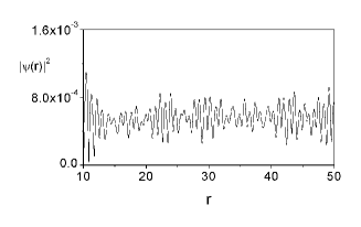
(a) (b) (c) (d) (e) (f) (g)

Figure 2: Configuration of the quasi-stabilized wavefunction. Parameters are the same as in previous figures. (a) A snapshot of an amplitude profile. (b) Tiny oscillations in the tail of the quasistabilized solution (c) Amplitude of the wavefunction far from the origin (the tail plus outgoing cylindrical wave). (d) Real part of the wavefunction far from the origin multiplied by $\sqrt{r}$. (e) Snap-shot of the phase factor of the quasi-stabilized solution. It can be seen that it is parabolic only at very small $r$. The curve has an inflection point at $r\leq 1$. f),g) The slowly decaying norm of the solution. Although the trap was turned off at $t=T_{off}=30$, the norm remains almost constant until the flux of atoms leaking from the core soliton reach the edge of the mesh and begin to disappear. After that it decreases slowly.

Such kind of stabilization in 3D has also been reported Adhikari . The latter finding is, however, in some disagreement with other investigations on this topic (for example, Ref. Abdullaev1 ). In Ref. 3D it was shown that the scattering length modulation may indeed provide for the stabilization in 3D, but only in combination with a quasi-1D periodic potential. So 3D geometry might need additional careful examination. In the present paper we concentrate on quasi-2D case only, where also not everything is clear yet. Unlike conventional 1D solitons, higher-dimensional solitonic objects may decay. Therefore, it is interesting to investigate the following question: is there indeed a novel genuine breather solution behind the phenomenon of stabilization? As we show in this paper, it turns out that the phenomenon does not fit into simple models being suggested earlier. For theoretical description of the process, several methods were used by different groups of authors: variational approximation based on the Gaussian anzatz Abdullaev1 ; SU , direct averaging of the GP equation Abdullaev1 , a method based on modulated Townes soliton Abdullaev1 , and the method of moments Garcia . Surprisingly, we find all the methods are not very satisfactory even for qualitative predictions. In brief, the direct averaging of the GP equation has the disadvantage of ommiting terms which are of the same order as those responsible for creation of the effective potential, while three other methods, although very different, all rely on the unwarranted assumption of parabolic dependence of the phase of the stabilized wavefunction on $r$: arg $\psi=\alpha(t)+\beta(t)r^{2}$. We find that the behavior of the exact numerical wavefunction is, however, completely different (see Fig. 2). The above-mentioned parabolic approximation (PA) of the phase factor is very popular because it is appealingly simple and indeed often appears in solutions of the time-dependent GP equation Kagan . Usually it comes from self-similar time evolution of the condensate density, for example in 3D the following dynamics of the condensate density is possible $\rho(x,y,z)=[\lambda_{1}(t))\lambda_{2}(t)\lambda_{3}(t)]^{-1}\rho(x/\lambda_{1}(t),y/\lambda_{2}(t),z/\lambda_{3}(t))$ , where coefficients $\lambda_{i}$ are coupled by nonlinear differential equations. It is the important finding of the present paper that in our problem a stabilized wavefunction does not have such parabolic phase factor and does not fit into self-similar patterns implied by the above-mentioned methods. This qualitative difference between the exact numerical solution and all theoretical models considered so far was not mentioned earlier. Besides, we noticed presence of steady outgoing flux of atoms in numerical stabilized solutions. So, even numerically there is no 2D soliton so far, but some slowly decaying object instead. Section 2 reviews the abovementioned theoretical methods. In Section 3 we give some results obtained using the variational approximation with non-gaussian trial functions, including ”supergaussian anzatz”. It is shown that a better accuracy can be obtained for predicting critical nonlinearity $g_{cr}$, but we were not able to determine accurately such dynamical properties as the frequency of slow oscillations. Additionally, we checked the supergaussian anzatz for another problem: determination of critical number of attractive BEC in a parabolic well, and found it to be much more accurate than the usual gaussian anzatz. This example also demonstrates that the stabilization mechanism is essentially more complicated than that assumed by the present (PA-based) methods, because predictions of the supergaussian anzatz for dynamical properties of the stabilized solution are much less accurate than in static problems.

In Section 4 numerical results are presented and compared with predictions of the theoretical methods discussed in Sections 2 and 3. Configuration of stabilized solution is discussed and dynamics of some integral quantities of the solution is investigated.

In Section 5 concluding remarks are given. We mention the relation between the BEC stabilization problem and stabilization of optical solitons in a layered medium with sign-alternating Kerr nonlinearity.

II Several approximate methods to study the problem: PA-based methods (Gaussian variational approximation, the modulated Townes soliton, the method of moments), and the direct averaging of the GP equation.

II.1 PA-based methods

II.1.1 Gaussian variational approximation

The variational approach based on the Gaussian approximation (GA) is one of the most often used in studying dynamics of the GP equation. In actual calculations this approximation however often gives a large error as compared to exact numerical results Metens ; Abdullaev2 . For example, in Ref. Metens the Gaussian approximation in dynamics of attractive BEC was compared to exact numerical solution of the GP equation. It was found that in estimating the critical number ${\cal N}_{c}$ of the condensate (the maximal number of condensed particles in a trap before collapse occurs) the Gaussian approximation gives a 17% error, and similar values of discrepancy for other dynamical quantities (as a useful test, in the Appendix we provide corresponding results obtained with a supergaussian variational ansatz). However, it seems that in this example GA enables to reproduce important features of the system at least qualitatively. The GA was also used in many other treatments of the GP equation using a variational technique. In particular, it was applied to the problem of BEC stabilization by the oscillating scattering length. The Lagrangian density corresponding to the GP equation (1) is

$$L[\psi]=\frac{i}{2}\left(\frac{\partial\psi}{\partial t}\psi^{*}-\frac{\partial\psi^{*}}{\partial t}\psi\right)-\frac{1}{2}\left|\frac{\partial\psi}{\partial r}\right|^{2}-\frac{1}{2}g(t)|\psi|^{4}.$$ (2)

The normalization condition for the wavefunction is $2\pi\int_{0}^{\infty}|\psi|^{2}rdr=1$.

In Ref. SU , a variational method with the following Gaussian anzatz was used,

$$\psi(r,t)=\frac{1}{\sqrt{\pi}R(t)}\exp\left[-\frac{r^{2}}{2R^{2}(t)}+i\frac{\dot{R}(t)}{2R(t)}r^{2}\right],$$ (3)

where $R(t)$ is the variational parameter that characterizes the size of the condensate, and the phase factor of the wavefunction describes the mass current SU ; AB ; Cirac .

After substitution of expression (3) into the Lagrangian density (2) one obtains the effective Lagrangian $L=2\pi\int_{0}^{\infty}rL[\psi]dr$ and the corresponding Euler-Lagrange equations of motion. One can obtain then the equation of motion for $R(t)$ as

$$\ddot{R}(t)=\frac{1}{R^{3}(t)}+\frac{g_{0}+g_{1}\sin{\Omega t}}{2\pi R^{3}(t)}.$$ (4)

So the gist of the model is to represent the 2D BEC as a classical nonlinear pendulum with modulated parameters. It is important that other one-parameter PA-based anzatzes also give the same nonlinear pendulum ($\ddot{R}=(a+b\sin\Omega t)/R^{3}$, where $a,b$ depend on the parameters $g_{1},g_{0},\Omega$), but with different functional dependence of a,b on the parameters.

The authors of Ref. SU use then the Kapitza averaging method to study behavior of the system with the rapidly oscillating scattering length. They assume the dynamics of $R$ can be separated into a slow part $R_{0}$ and a small rapidly oscillating component $\rho$: $R=R_{0}(t)+\rho(\Omega t)$. From the equations of motion for $R_{0}$ and $\rho$ one extracts the effective potential for the slow variable $U(R_{0})\approx\frac{A_{2}}{R_{0}^{2}}+\frac{A_{6}}{R_{0}^{6}}$ and determines its minimum

$$R_{min}=\left(\frac{-3}{4\pi(g_{0}+2\pi)}\right)^{1/4}\left(\frac{g_{1}}{\Omega}\right)^{1/2}.$$ (5)

From the expression for the effective potential for $R_{0}$ they obtained dependence of the monopole moment $<r>$ and the breathing-mode frequency $\omega_{br}$ on parameters $g_{1},\Omega$. The frequency of small oscillations (breathing mode) around the minimum is given by SU

$$\omega_{br}^{2}=\frac{8\Omega^{2}}{3g_{1}^{2}}(g_{0}+2\pi)^{2}.$$ (6)

Their numerical calculations were done for $g_{0}=-2\pi$. One can see that theoretical predictions (5) and (6) based on the Gaussian approximation can catch $(g_{1}/\Omega)^{1/2}$ dependence of the monopole moment $<r>$ and $(\Omega/g_{1})$ dependence of the breathing-mode frequency $\omega_{br}$ but cannot determine the corresponding coefficients of proportionality, of which the one in (5) becomes infinity while the one in (6) becomes zero for $g_{0}=-2\pi$, the value actually used in the numerical calculations. On the other hand, from numerical calculations they were able to determine the coefficients as $1.06$ and $0.32$ correspondingly (see Fig. 2 of Ref. SU ). It was also determined in Ref. SU that in order to stabilize the bright soliton, $|g_{0}|$ must exceed the critical value of collapse $|g_{cr}|$. Their numerical estimate for $|g_{cr}|$ is $\approx$ 5.8 while theoretical estimate based on Gaussian approximation is $2\pi\approx 6.28$. The $2\pi$ estimate in fact corresponds to fitting the so-called Townes soliton by a Gaussian trial function as will be discussed below.

Inspired by the idea of comparing a numerical solution with simple model nonlinear pendulum, one may ask if it is possible to obtain a better accord with the numerical experiments using different ansatzes. We study this question in Section 3, and it seems that only the stationary Townes soliton can be fit accurately, but not the stabilized breather solutions.

II.1.2 Modulated Townes soliton

A method based on modulated Townes soliton used in Ref. Abdullaev1 ; Garcia should be mentioned. The Townes soliton is a stationary solution to the 2D NLS equation with constant nonlinearity $g_{cr}$. In our notations $|g_{cr}|\approx 1.862\pi\approx 5.85$. This solution is unstable: if $|g|$ is slightly increased or decreased, the solution will start to collapse or expand correspondingly. If the value of $g$ is close to $g_{cr}$, one may search for a solution of the problem with fast oscillating $g$ in the form of a modulated Townes soliton, as described in Refs. Abdullaev1 ; Garcia . A solution is sought in the form of

$$\Psi(r,t) \approx [a(t)]^{-1}R_{T}[r/a(t)]e^{iS},$$

$$\quad S = \sigma(t)+\frac{r^{2}\dot{a}}{4a},\quad\dot{\sigma}=a^{-2},$$ (7)

where $R_{T}$ represents amplitude of the Townes soliton. Then, starting from the approximation (7), one can derive the evolution equation for $a(t)$ and so determine the dynamics of the system. Note that the approach is also PA-based. It is inevitable if we are to use one-parameter self-similar trial function in the form of $|\psi(r,t)|=Af(r/a,t)$.

II.1.3 The method of moments

Another PA-based method we would like to mention here is the method of moments Garcia . One introduces integral quantities $I_{1},I_{2},I_{3},..$ as

$$I_{1} = \int_{0}^{\infty}|\psi|^{2}d{\bf r},\qquad I_{2}=\int_{0}^{\infty}r^{2}|\psi|^{2}d{\bf r},$$

$$I_{3} = i\int_{0}^{\infty}\left(\psi\frac{\partial\psi*}{\partial r}-\psi^{*}\frac{\partial\psi}{\partial r}\right)rd{\bf r},$$ (8)

$$I_{4} = \frac{1}{2}\int_{0}^{\infty}\left(|\nabla\psi|^{2}+\frac{n}{2}g(t)|\psi|^{4}\right)d{\bf r},$$

$$I_{5} = \frac{n}{4}\int_{0}^{\infty}|\psi|^{4}d{\bf r},$$

where $n=2,3$ is the dimension of the problem. In 2D, $d{\bf r}=2\pi rdr$, and in 3D $d{\bf r}=4\pi r^{2}dr$.

For all t, we have $I_{1}=1$. For the remaining $I_{i}$ one can write down the dynamical equations of motion as Garcia :

$$\dot{I_{2}}=I_{3},\quad\dot{I_{3}}=I_{4},\quad\dot{I_{4}}=g\frac{n-2}{n}I_{5}+\dot{g}I_{5},$$ (9)

$$\dot{I_{5}}=\frac{n\pi 2^{n}}{8}\int_{0}^{\infty}\frac{\partial|\psi|^{4}}{\partial r}\frac{\partial\arg\psi}{\partial r}r^{n-1}dr$$ (10)

The system of equations for the momenta is not closed because of $I_{5}$, and one should make some approximation in order to close it. In Ref. Garcia it was assumed that

$$\arg\psi=\frac{I_{3}r^{2}}{4I_{2}},$$ (11)

i.e. the phase factor is proportional to $r^{2}$ (so that again it is a PA-based method) and the coefficient of proportionality is given by the ratio of $I_{3}$ and $I_{2}$. Then the system (9) poses dynamical invariants Garcia :

$$Q_{1} = 2(I_{4}-gI_{5})I_{2}-\frac{1}{4}I^{2}_{3},$$ (12)

$$Q_{2} = 2I^{n/2}_{2}I_{5}.$$ (13)

With the help of these invariants, the system becomes

$$\ddot{I}_{2}-\frac{1}{2I_{2}}\Bigl{(}\dot{I}_{2}\Bigr{)}^{2}=2\left(\frac{Q_{1}}{I_{2}}+g\frac{Q_{2}}{I^{n/2}_{2}}\right).$$ (14)

Introducing $X(t)=\sqrt{I_{2}(t)}$ one obtains Garcia

$$\ddot{X}=\frac{Q_{1}}{X^{3}}+g(t)\frac{Q_{2}}{X^{n+1}}.$$ (15)

The equation is analogous to that obtained by other PA-based methods. One can investigate the obtained equation (15) using various methods of nonlinear dynamics. The simplest Kapitza averaging method can be used again, but of course it is better to use rigorous averaging technique since modern averaging methods are available AKN which have been extensively used already in plasma physics, hydrodynamics, classical mechanics It1 . The authors of Ref. Garcia fulfilled rigorous analysis of model Eq. 15 using results of Ref. Ref_Garcia . It is important to have in mind that the relation between the exact dynamics of the full system and that of the model (15) of the method of moments remains unclear, therefore one cannot determine sufficient conditions for stabilization, etc. In Ref. Garcia it was noticed that the correspondence between numerical simulation of full 2D GP equation and dynamics of the model system (15) is not good. As it is seen from Fig. 3 of Ref. Garcia , neither the frequency of slow oscillations nor the position of the minimum of the effective potential is predicted correctly. Nevertheless, we found that in numerical stabilized solutions magnitudes of $Q_{1}$ and $Q_{2}$ are often well-conserved, i.e. they oscillate about some mean value (see Section 4).

II.2 Direct averaging of the GP equation

Ref. Abdullaev1 also explores the Gaussian variational approximation. Beside that, a very promising method of directly averaging the GP equation was investigated. It is based on an analogous method used for the one-dimensional NLSE with periodically managed dispersion (in the context of optical solitons) Kath . In Ref. Abdullaev1 the solution is sought as an expansion in powers of $1/\Omega$ (in our notation):

$$\psi(r,t)=A(r,T_{k})+\Omega^{-1}u_{1}(A,\zeta)+\Omega^{-2}u_{2}(A,\zeta)+....,$$ (16)

with $<u_{k}>=0$, where $<...>$ stands for the average over the period of the rapid modulation, $T_{k}\equiv\Omega^{-k}t$ are the slow temporal variables ($k=0,1,2,...$), while the fast time is $\zeta=\Omega t$. Then, for the first and second corrections the following formulas were obtained:

$$u_{1} = -i[\mu_{1}-<\mu_{1}>]|A|^{2}A,$$

$$\quad\mu_{1} \equiv \int_{0}^{\zeta}[g(\tau)-<g_{1}>]d\tau,$$ (17)

$$u_{2} = [\mu_{2}-<\mu_{2}>][2i|A|^{2}A_{t}+iA^{2}A^{*}_{t}+\Delta(|A|^{2}A)]$$

$$- |A|^{4}A(\frac{1}{2}[(\mu_{1}-<\mu_{1}>)^{2}-2M]+$$

$$+ <g>(\mu_{2}-<\mu_{2}>))],$$

$$\quad\mu_{2} = \int_{0}^{\zeta}(\mu_{1}-<\mu_{1}>)ds,\quad M=\frac{1}{2}(<\mu_{1}^{2}>-<\mu_{1}>^{2}).$$

Using these results, the following equation was obtained for the slowly varying field $A(r,T_{0})$, derived up to the order of $\Omega^{-2}$:

$$-i\frac{\partial A}{\partial t} = \Delta A+|A|^{2}A+2M\left(\frac{g_{1}}{\Omega}\right)^{2}[|A|^{6}A$$

$$-3|A|^{4}\Delta A + 2|A|^{2}\Delta(|A|^{2}A)+A^{2}\Delta(|A|^{2}A^{*})].$$

The above equation was represented in the quasi-Hamiltonian form

$$\Bigl{[}1 + 6M\left(\frac{g_{1}}{\Omega}^{2}|A|^{4}\right)\Bigr{]}\frac{\partial A}{\partial t}=-\frac{\delta H_{q}}{\delta A^{*}},$$

$$H_{q} = \int dV\Bigl{[}|\nabla A|^{2}-2M\left(\frac{g_{1}}{\Omega}\right)^{2}|A|^{8}$$ (19)

$$- \frac{1}{2}|A|^{4}+4M\frac{g_{1}}{\Omega}|\nabla(|A|^{2}A)|^{2})^{2}\Bigr{]}.$$

However, some contribution was missed while deriving Eq. (LABEL:slow). Let us take into account the third correction $u_{3}(A,\zeta)$:

$$\psi(r,t) = A(r,T_{k})+\Omega^{-1}u_{1}(A,\zeta)+\Omega^{-2}u_{2}(A,\zeta)$$ (20)

$$+ \Omega^{-3}u_{3}(A,\zeta)+....$$

Then, up to terms of order $\Omega^{-2}$ it changes nothing in r.h.s of Eq.(LABEL:slow) (spatial part), but it adds to l.h.s. of Eq. (LABEL:slow) an undetermined term $\Omega^{-2}\partial u_{3}/\partial\zeta$ . This term has the same order $\Omega^{-2}$ as the terms from the second correction. So we do not get here a consistent equation for the slow field $A$ because we do not have a closed set of equations for the second-order corrections (third order correction becomes second order correction after differentiating in time), and so the quasi-Hamiltonian (19) contains an undetermined error of the second order in $\Omega^{-1}$. The influence of the contribution is not very clear but require additional investigation. Nevertheless, formally the omitted terms have the same order as those responsible for the creation of the effective potential. Having in mind how many difficulties arise in averaging of systems of ordinary differential equations AKN , the rigorous direct averaging of the GP equation constitutes a very interesting and challenging open problem, since in principle it could reveal a true periodic solutions in such oscillating objects.

III Variational approximation with non-Gaussian ansatzes

Here we try to investigate the system more accurately using some non-Gaussian ansatzes and see if it is possible to get more accurate theoretical estimates. One may be interested in three dynamical quantities of the system: the value of critical nonlinearity $g_{cr}$, slow frequency of breathing oscillations of the stabilized soliton $\omega_{br}$, and minimum of the effective potential $R_{min}$ about which the expectation value of the monopole moment $<r>$ oscillates slowly.

Table 1 summarizes results of variational predictions for the critical nonlinearity $g_{cr}$ and frequency of small breathing oscillations using several different ansatzes. Note that the phase dependence of a one-parameter trial function is not important for calculating $g_{cr}$. It is understood that if we choose a trial wavefunction with its amplitude in the form of $|\psi(r,t)|=Af[r/a(t)]$, then we need to use a phase factor with quadratic $r-$ dependence in order for the ansatz to be self-consistent (i.e., the mass current generated by the changing parameter would be incorporated in the phase factor of an ansatz). On the other hand, since amplitude part of the trial function is just an approximation, one may try to use other forms of phase factor with the same functional form of the amplitude.

When predicting the frequency of breathing oscillations from the corresponding effective potential, it is easy to obtain the result for small amplitude linear breathing oscillations (given in Table 1), but in actual stabilized solutions amplitudes of breathing oscillations are not so small.

It is possible to take into account anharmonicity of breathing oscillations. As was mentioned earlier, all PA-based anzatzes produce the nonlinear pendulum $\ddot{R}+(a+b\sin\Omega t)/R^{3}$, with a corresponding effective potential having $R_{min}=\left(-\frac{3b^{2}}{2\Omega^{2}a}\right)^{1/4}$ , $\omega_{br}=\sqrt{\frac{8}{3}}\Omega|a/b|,$ where $\omega_{br}$ is the frequency of the small amplitude breathing oscillations (near the bottom of the effective potential). For larger breathing oscillations the (anharmonic) breathing frequency will be amplitude-dependent: $\omega_{br}^{anh}=2\pi\left(\sqrt{-\frac{2}{h}}\left[\frac{x_{3}}{\sqrt{x_{2}-x_{3}}}\mbox{\bf K}(k)+\frac{x_{2}}{x_{1}}\sqrt{x_{2}-x_{3}}\mbox{\bf E}(k)\right]\right)^{-1}$, with $\quad k=\sqrt{\frac{x_{2}-x_{1}}{x_{2}-x_{3}}},$ where $x_{1}=R_{1}^{2}$, $x_{2}=R_{2}^{2}$ ($R_{1},R_{2}$ being the turning points), $x_{3}$ is the third root of the equation $h=\frac{a}{2x}+\frac{b}{4\Omega^{2}x^{3}}$. The magnitudes of $x_{1},x_{2},x_{3},h$ can be determined from numerically obtained breathing oscillations (but results depend on the choice of a particular anzatz). Even this improvement is not helpful, simply because the parabolic approximation is not valid.

Finding $g_{cr}$ only might be considered as an approximation to the stationary Townes soliton by a trial function so that the mass current term equals zero and that a phase factor may be skipped from the calculations. It is known that the Townes soliton $\psi_{t}=e^{it}R_{T}(r,t)$ at large $r$ has asymptotic behavior for its amplitude in the form $R_{T}\sim e^{-r}/\sqrt{r}$ . So that Gaussian ansatz is not very good for finding $g_{cr}$ just because it is decaying too fast at large $r$. The supergaussian trial function provide a better approximation, namely $g_{cr}=\pi 2^{\frac{1}{\mbox{ln}2}}\mbox{ln}2$ which corresponds to the supergaussian wavefunction with $\eta=\eta_{T}=2\mbox{ln}2<2$. Previously the supergaussian ansatz was used to fit stationary solutions of some nonlinear problems including NLS equation in the context of BECs Pramana . The superposition of two Gaussians in the form $A\exp(-\frac{r^{2}}{2R^{2}})\mbox{Cosh}(\gamma\frac{r^{2}}{2R^{2}})$ also enables one to obtain some improvement: $g_{cr}\approx 5.883$. The Secanth ansatz

$$\psi=\frac{A}{\cosh(r/R)}\exp[iS(\dot{R},R)r^{2}]$$

works better, with only one parameter it overcomes the above-mentioned two-parameter trial functions. A very good approximation is provided by the simplest ansatz among all considered:

$$\psi=\frac{1}{3R\sqrt{\pi}}\left(1+\frac{r}{2R}\right)\exp\left\{-\frac{r}{2R}+iS(\dot{R},R)r^{2}\right\}.$$ (21)

It fits the Townes soliton adequately both at the origin and asymptotically at infinite $r$ ( a pre-exponential multiplier is not so important as the exponential factor ). The pre-exponential factor is needed in order to fulfill the boundary condition in the origin $\lim_{r\to 0}\frac{1}{r}\psi_{r}<\infty$ . Note that in the supergaussian ansatz the former condition is not fulfilled, otherwise (if one included it in a similar way) the result would be better at the cost of more bulky calculations. The accuracy of the prediction implies that ansatz (21) provides a very good approximation to the Townes soliton at fixed $R$, and could approximately represent the modulated Townes soliton when $R$ is time-dependent and the phase factor with parabolic $r-$dependence is used in accordance with the continuity condition.

Table 1: Variational predictions for the properties of stabilized solutions.

Ansatz	Amplitude part	$g_{cr}$,	$g_{cr}$,	$\kappa_{br}$
	of the anzatz	analytical	approximate	(linear prediction,
		expression	value	$\omega_{br}=\kappa_{br}\Omega/g_{1}$)
Gaussian	$A\exp(-\frac{r^{2}}{2R^{2}})$	2 $\pi$	6.283	$\sqrt{\frac{8}{3}}(g_{0}+2\pi)$
Supergaussian	$A\exp(-\frac{1}{2}\Large(\frac{r}{R}\Large)^{\eta})$	$\pi 2^{\frac{1}{\mbox{ln}2}}$ ln2	5.919
Secanth	$A\mbox{Sech}\Large(\frac{r}{R}\Large)$	$2\pi\ln{2}\frac{2\mbox{ln}2+1}{4\mbox{ln}2-1}$	5.863	$\sqrt{\frac{8}{3}}\frac{|2\ln 2+1+g_{0}(\frac{4\ln 2-1}{2\pi\ln 2})|}{\frac{4\ln 2-1}{2\pi\ln 2}}$
Exponential	$A(1+\frac{r}{2R})\exp(-\frac{r}{2R})$	$\frac{144}{77}\pi$	5.875

After obtaining estimates for $g_{cr}$, one can use the above-mentioned ansatzes in order to find an effective potential, its minimum and frequency of the breathing oscillations of the monopole moment about this minimum in the same way as it was done for the Gaussian ansatz. We checked the Sech ansatz and the supergaussian with quadratic phase dependence. In the supergaussian ansatz the parameter $\eta$ was fixed at the value of its ”Townes soliton-like” solution $\eta=\eta_{T}=2\mbox{ln}2$. In such a way the variational approximation with supergaussian ansatz resembles method of modulated Townes soliton. However, we find that such trial function seriously underestimate minimum of the effective potential (i.e. the mean value about which the monopole moment oscillates). Nevertheless, the result of the Gaussian ansatz is even worse since for $g_{0}=2\pi$ it gives the diverging expression for $R_{min}$ and zero for frequency of slow breathing oscillations $\omega_{br}$, as mentioned in Section 1 and SU . A natural idea for remedy is to use two-parameter trial functions to reproduce the non-parabolic phase factor dependence on $r$. In the supergaussian ansatz it can be done by considering $\eta$ as a dynamical (time-dependent) parameter. The problem is that it is difficult to obtain the self-consistent expression for the phase factor. We also try the supergaussian ansatz with fixed $\eta$ and with non-quadratic phase dependence (which is unfortunately not self-consistent trial function) $\psi(r,t)=A\exp\left[-\frac{(a+ib)r^{\eta_{T}}}{2}\right],$ where $A,a,b,$ and $\eta$ are all functions of time, parameter $\eta$ is fixed at the value of its Townes soliton-like solution $\eta=\eta_{T}=2\mbox{ln}2$. We find that such modification drastically changes dynamical parameters of the system. Still, the resulting model is the same classical nonlinear pendulum as in the Gaussian approximation, but with different parameters. The rigorous way to employ the two-parameter supergaussian ansatz is to let $\eta$ be a dynamical variable and construct a phase factor fulfilling continuity condition for the trial function. One could then obtain the two-dimensional effective potential within the same Kapitza approach.

As a useful test of applicability of the supergaussian anzatz, we determine the critical number of attractive BEC in the 3D parabolic trap studied in Ref. Metens . Their numerical result was $N_{cr}=1258.5$, while the gaussian approximation yields $N_{cr}^{G}=1467.7$. We found the supergaussian prediction to be very accurate $N_{cr}^{SG}=1236.1$.

IV Numerical results

Numerical calculations reveal the fact that stabilized solutions do not have parabolic phase factors in contradiction to all the methods considered in Section 2 (except the method of direct averaging). The calculations were done using explicit finite difference schemes. We use explicit finite differences of second and forth order for spatial derivatives and 4-th order Runge-Kutta method for time propagation. We use meshes varying from 2000 to 10000 points, timesteps $\Delta t=0.0001\sim 0.0004$, and spatial steps $\Delta r=0.02\sim 0.04$. In addition, we found that it is very important to use absorbing (imaginary) potential at the edge of the mesh, in accordance with the conclusions of Ref. Garcia . Without such an adsorbing potential, a wave reflected from the edge sometimes destroys the otherwise stable solution.

Following SU , initially we start with a Gaussian wavepacket in a parabolic trap. Then the trap was slowly turned off while the oscillating nonlinearity was slowly turned on in a way similar to Ref. SU . In Figure 1 one can see indeed the creation of a stabilized soliton. In Figure 1b and 1d oscillations of amplitude of the wavefunction at the origin are shown. It decays very slowly. In fact, this is in accord with the calculations of Ref. SU : after a careful examination of the corresponding figures in that paper one notices the same behavior. Monopole moment grows very slowly (Figs. 1a,c). We checked that in the case when the trap is not turned off completely, the norm is conserved during the same long time with a high accuracy (of order $10^{-8}$), so decay is certainly not due to numerical errors.

In Fig. 2 configuration of the quasi-stabilized wavefunction is shown. One can see the smooth core pulse profile, tiny oscillations in the tail, and an outgoing cylindrical wave leaking from the core pulse. In Fig. 2e the behavior of the phase factor is shown. It is seen to differ from parabolic with $r$ considerably.

Figs. 2f,g shows the slow decay of the norm of the solution due to the flux of atoms from the core to infinity. We made a series of numerical experiments with different parameters. We found that the behavior of the matter-wave pulse is often unpredictable. When the Gaussian approximation predicts stabilization, in the corresponding numerical solution it does not necessarily occur. Neither can the method of moments give reliable predictions for the stabilization. We checked the latter method carefully. As it was mentioned already in Sections 1 and 2, the method relies on the crucial approximation of Eq. (11 ). It is due to this approximation one obtains the existence of dynamical invariants $Q_{1}$ and $Q_{2}$ (see Eq. 13). As a result, dynamics is determined by Eq. (15). Returning back to Figure 2, we see a snapshot of the phase factor, arg $\psi$, of a stabilized solution. It clearly demonstrates that none of the PA-based methods reproduce the dynamics of the system adequately. Only at small $r$ the parabolic law is fulfilled, while the deviation from this quadratic dependence is very strong even at $r\leq 1$, where the amplitude of the solution is not small at all (and is sufficient to drastically influence the dynamics of the system). Snapshots at other moments produce similar results: the phase of the solution is changing with time but remains very far from being parabolic in $r$. It is easy to check that dynamical properties of the system within a variational approximation are very sensitive to $r-$ dependence in the phase factor of a trial function. To check the dynamics further, we calculated time evolution of the ”invariants” $Q_{1}$ and $Q_{2}$ in the stabilized solution. They are constants in the model but not in the exact numerical solution. We found that in the numerical quasi-stabilized solution these magnitudes oscillate around some mean value. Actually, it was already found in Ref. Garcia that the method of moments does not work for Gaussian initial data, still it is interesting to trace dynamics of relevant magnitudes. The time evolution of $Q_{1}$ and $Q_{2}$, and other magnitudes related to the method of moments are shown in Figures 4, and 5. It is seen that the magnitudes of $Q_{1}$ and $Q_{2}$ related to a stabilized soliton undergo slow oscillations.

When calculating values of $Q_{1}$ and $Q_{2}$, and other properties of the quasi-stabilized solution it is necessary to stop integration at some reasonable value of $r=r_{max}$ (we take $r_{max}=20$ where the amplitude of the wavefunction becomes very small (of order $10^{-4}$ in our case). In that way we separate the properties of the quasi-stabilized soliton from that of the tail which, although has very small amplitude, can carry large moments $I_{2},I_{3}$ and would give large contribution to $Q_{1}$ and $Q_{2}$ (so that in the corresponding figures we presented these quantities for the core soliton and the whole solution (including tail) separately).

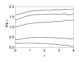
(a) (b) (c) (d) (e) (f) (g)

Figure 6: Oscillations of the monopole moment of a quasistabilized solution. Parameters are $g_{0}=-7.0$, $\Omega=40$, $g_{1}=8\pi$ . Initial frequency of the parabolic trap was chosen to be $\omega(0)=4.0$. (a) Time evolution of the monopole moment on very long time. (b) Detailed picture of the time evolution of the monopole moment of a quasistabilized solution about $t\approx 600$.(c) Detailed picture of the time evolution at $t=1800\sim 2000$. (d) Decaying norm of the solution. (e) Time evolution of the integral quantity $Q_{1}$ (calculated for the core part of the wavefunction) (f) Time evolution of $Q_{2}$. (g)Several snap-shots of the phase factor of the quasi-stabilized solution (made at different moments). Note that typical behavior of the phase factor is not quadratic with $r$ at all.

Similar features can be seen in Fig. 6 where calculations with $g_{0}=-7.0$ are presented. Several snapshots of the phase factor at different moments are presented in order to demonstrate that non-quadratic behavior of the phase factor is typical. Time evolution on very long time is traced. We find that sometimes magnitudes of $Q_{1}$ and $Q_{2}$ of stabilized solutions are almost conserved (undergoing small oscillations about its mean value) despite the strongly non-quadratic behavior of the phase factor. It suggests that the method of moments developed in Garcia might provide useful perspective for studying the problem and it would be fruitful to extend it taking into account non-parabolicity of the phase factor.

V Concluding remarks

Despite there are many publications dedicated to the stabilization of a trapless BEC by the rapidly oscillating scattering length, it seems that the strong non-parabolic behavior of the phase of the stabilized wavefunction has not been brought to attention yet. It should be noted that the role of deviation of the phase profile of NLSE solutions from the parabolic shape was addressed previously in the contexts of solitons in optical fibers in Refs. nonparabolic1 ; nonparabolic2 .

Despite that several independent methods were used previously, we have seen that three of the four theoretical methods used rely on the unwarranted parabolic approximation, while the fourth method (direct averaging of GP equation) is, strictly speaking, incorrect, despite its inspiring motivation (in the sense that the omitted terms has the same order as those responsible for the creation of the effective potential ). Besides, we find that there is no evidence presently for stabilization in a strict sense. It seems that the numerical examples presented so far deal with quasi-stable solutions which slowly decays due to the leaking of atoms from the core pulse as an outgoing cylindrical wave. It means that even from a numerical point of view there are no evidence for true 2D solitons (breathers) yet.

It should be mentioned also that the phenomenon of BEC stabilization has its counterpart in nonlinear optics. As was studied in Ref. Towers , in the periodically alternating Kerr media the stabilization of beams is possible. Mathematically, one deals with a similar NLSE. Instead of the time-dependence of the scattering length of BEC one has dependence of the media nonlinearity coefficient on the coordinate z along which a beam propagates:

$$iu_{z}+\frac{1}{2}\nabla_{tr}^{2}u+\gamma(z)|u|^{2}u=0,$$ (22)

where the diffraction operator $\nabla_{tr}^{2}$ acts on the transverse coordinate $x$ and $y$. Nonlinearity coefficient $\gamma(z)$ jumps between constant values $\gamma_{\pm}$ of opposite signs inside the layers of widths $L_{\pm}$. The analysis of this problem was done using variational approximation based on a natural Sech ansatz $U=A(z)\exp[ib(z)r^{2}+i\phi(z)]\mbox{Sech}[r/w(z)]$. However, behavior of the phase factor was not checked aposteriori . We see that it would be useful to investigate the problem of (2+1)-dimensional solitons in a layered medium with sign-alternating Kerr nonlinearity in a greater detail because behavior of the phase factor of the numerical solution has not been reported yet. Interplay between the phenomenon of stabilization in Kerr media and BEC was addressed also in Ref. Adhikari2 in the context of stabilization of (3+1)- dimensional optical solitons and BEC in periodic optical-lattice potential (without addressing the issue of validity of the parabolic approximation).

Returning back to the BEC stabilization, we note that the two main difficulties should be resolved in the future: the non-trivial behavior of the argument of the stabilized wavefunction, and the possibility to stop the leak of atoms from the tail of the solution.

Using several non-Gaussian variational functions, we were able to determine accurately one of the magnitudes characterizing the stabilization phenomena: critical nonlinearity $g_{cr}$, but not other dynamical properties such as the frequency of slow oscillations.

VI Acknowledgements

Alexander Itin (A.I.) acknowledges support by the JSPS fellowship P04315. A.I. thanks Professor Masahito Ueda and Professor S.V. Dmitriev for helpful discussions.

This work was supported in part by Grants-in-Aid for Scientific Research No. 15540381 and 16-04315 from the Ministry of Education, Culture, Sports, Science and Technology, Japan.

(a) (b) (c) (d) (e)

Figure 1: (a)Oscillations of the monopole moment after turning off the trap. Parameters are $g_{0}=-2\pi$, $g_{1}=8\pi$, $\Omega=30$. The trap was turned off completely at $T_{off}=30$. (b) Time evolution of amplitude of wavefunction at the origin. (c) Oscillations of the monopole moment on longer time scale. (d) Time evolution of amplitude of wavefunction at the origin on longer times. (e) The oscillations of the monopole moment from previous figure on finer scale. Tiny high frequency oscillations are seen.

(a) (b)

Figure 3: Oscillations of the monopole moment. (a) $g_{0}=-6.5$, $\Omega=35$, $g_{1}=10\pi$ . Initial frequency of the parabolic trap is $\omega(0)=0.8$. (b) $g_{0}=-6.5$, $\Omega=30$, $g_{1}=14.5$ . Initial frequency of the parabolic trap is $\omega(0)=1$. Quasistabilized solution is destroyed after several oscillations.

(a) (b) (c) (d)

Figure 4: Time evolution of the integral quantities $Q_{1},Q_{2}$. (a) Oscillations of ”shortened” $\mbox{Q}_{2}$ (designated as $q_{2}$). We integrate expressions entering Eq. (13) from $r=0$ to $r\approx 8$ so that it characterizes the core part of the solution (quasi-stabilized soliton) without the oscillating tail. (b) Time evolution of full $Q_{2}$. The expressions (13) were integrated from $r=0$ to $r\approx 120$ so that it includes large contribution from the oscillating tail. (c) Time evolution of ”shortened” $\mbox{Q}_{1}$ (designated as $\mbox{q}_{1}$). We integrate expressions entering Eq. (13) from $r=0$ to $r\approx 8$ so that it characterizes the core part of the solution. Dynamics of the core soliton for quite a long time is almost independent of the behavior of the tail which after reaching the edge of the grid begin to disappear. (d) Time evolution of the full $Q_{1}$ (including large contribution from the oscillating tail which depends on location of the absorbing potential and the mesh size ).

(a) (b) (c) (d)

Figure 5: Time evolution of the moments ($I_{2},I_{3},I_{4}$). (a) Oscillations of the second moment $<r^{2}>$ of the core soliton (designated as $i_{2}$). The boundary of the core of the quasi-stabilized soliton was taken to be $r\approx 8$. (b) Time evolution of the second moment $I_{2}=<r^{2}>$ of the whole solution including tail (this magnitude depends on mesh size, here $r_{max}\approx$ 120) (c) Time evolution of $I_{4}$. (d) Time evolution of $I_{3}$.