Resonant x-ray scattering spectra from multipole orderings:
Np M_4,5 edges in NpO₂

Abstract

We study resonant x-ray scattering (RXS) at Np M_4,5 edges in the triple-k multipole ordering phase in NpO₂, on the basis of a localized electron model. We derive an expression for RXS amplitudes to characterize the spectra under the assumption that a rotational invariance is preserved in the intermediate state of scattering process. This assumption is justified by the fact that energies of the crystal electric field and the intersite interaction is smaller than the energy of multiplet structures. This expression is found useful to calculate energy profiles with taking account of the intra-Coulomb and spin-orbit interactions. Assuming the $\Gamma_{8}$-quartet ground state, we construct the triple-k ground state, and analyze the RXS spectra. The energy profiles are calculated in good agreement with the experiment, providing a sound basis to previous phenomenological analyses.

I Introduction

Resonant x-ray scattering (RXS) technique has attracted much attention to study spin and orbital properties of 3d transition-metal compounds. RXS at the $K$-edge is described by a second-order optical process that an incident x-ray excites a $1s$ core electron to unoccupied $4p$ states and then the $4p$ electron is recombined with the core hole with emitting x-ray in the dipole process ($E1$). It became widely known after the observation of intensities on orbital-ordering superlattice spots at Mn K-edge in LaMnO₃.Murakami et al. (1998) At the earlier stage, the spectra were interpreted as a direct observation of orbital ordering.Ishihara and Maekawa (1998) However, subsequent theoretical studies based on band structure calculations revealed that the spectra are a direct reflection of lattice distortion,Elfimov et al. (1999); Benfatto et al. (1999); Takahashi et al. (1999) since the $4p$ state in the intermediate state is influenced not by the orbital ordering of $3d$ electrons but by lattice distortion through the hybridization with the $2p$ state at neighboring oxygen sites.

Different from transition-metal compounds, M_4,5 edges are available for forbidden reflection Bragg spots in actinide compounds.Isaacs et al. (1990); Mannix et al. (1999); Longfield et al. (2002) The RXS spectra are more directly reflecting multipole orderings of $5f$ states, since the $E$1 process involves a transition from the $3d$-core to $5f$ states. Each actinide atom usually carries local multipole moments, which can order at low temperatures due to intersite interactions such as exchange interactions. For such localized electron systems, RXS amplitudes are given by summing up contributions at each site. The crystal electric field (CEF) and the intersite interaction can be safely neglected in the intermediate state, because they are much smaller than the intra-atomic Coulomb interaction. Therefore, it may be reasonable to assume that the intermediate state preserves the rotational invariance. Under the assumption, we derive an expression for the RXS amplitude in the $E$1 process to characterize the spectra. Although the expression is essentially the same as the formula by Hannon et al.,Hannon et al. (1989) the present form is useful to calculate energy profiles with taking full account of multiplet structures. Using this expression together with a microscopic model, we calculate the RXS spectra in the triple-k multipole ordering phase in NpO₂.

NpO₂ undergoes a second-order phase transition below $T_{\textrm{0}}=25.5$ K. Osborne and E. F. Westrum (1953); Erdös et al. (1980) Since Np ions are Kramers ions in the $(5f)^{3}$ configuration, a magnetic ground state is naturally expected. However, neither Mössbauer spectroscopyDunlap et al. (1968); Friedt et al. (1985) nor neutron diffraction experimentsCox and Frazer (1967); Heaton et al. (1967) could detect any evidence of the sizable magnetic moment. Actually, the former experiment gave an estimate of the upper limit of the magnitude of the magnetic moment $\sim 0.01\mu_{\textrm{B}}$, which was too small to explain the effective paramagnetic moment $\sim 2.95\mu_{\textrm{B}}$.Ross and Lam (1967) Another complication is that a muon spin relaxation ($\mu$SR) experiment has suggested the low-temperature phase of breaking time-reversal symmetry.Kopmann et al. (1998)

A natural way to reconcile with the above observations is to introduce the higher-rank multipole ordering rather than the dipole moment. Actually, Santini and Amoretti proposed a octupole ordering of $\Gamma_{2}(xyz)$ symmetry.Santini and Amoretti (2000, 2002) However, this phase can be ruled out because it gives rise to no RXS intensity. Recently, Paixão et al. have reported that a longitudinal triple-k octupole ordering accounts well for their RXS experiment.Paixão et al. (2002) The reason for anticipating triple-k orderings is that it excludes a crystal distortion or a shift of oxygen positions, which is consistent with the experiment. Experimental data obtained from the ¹⁷O NMR spectrum, which indicate the existence of two inequivalent oxygen sites, support the occurrence of the triple-k octupole ordering phase.Tokunaga et al. (2005) Some theoretical works also have lent support to realization of this type of the phase.Kiss and Fazekas (2003); Kubo and Hotta (2005)

Assuming the $\Gamma_{8}$-quartet ground state, we explicitly construct a triple-k octupole ordering state. This state is found to simultaneously carry a finite quadrupole moment, which generates the RXS intensity. Since the RXS amplitudes are characterized by three terms, the scalar, dipole, and quadrupole ones, it is not necessary to assume the existence of the hexadecapole moment instead of the quadrupole moment. We calculate the energy profiles with taking full account of multiplet structures in the intermediate state. We obtain spikes-like curves at Np $M_{4}$ edges for smaller values of the core-level width $\Gamma$ as a reflection of multiplet structures. They are found to merge into a single peak with $\Gamma>1$ eV. The energy profile with $\Gamma\sim 2$ eV seems to agree with the experiment. The azimuthal-angle dependence of the RXS spectra is obtained in agreement with the previous analysis.Paixão et al. (2002); Caciuffo et al. (2003) The present analysis provides a sound basis to the previous phenomenological analysis.

The present paper is organized as follows. In Sec. II, we present an expression for the RXS amplitude, which is useful to calculate the energy profiles. In Sec. III, we analyze the RXS spectra in the triple-k octupole ordering of NpO₂ on the basis of a localized electron model. Section IV is devoted to concluding remarks. In Appendix, we derive the general expression of RXS characterizing energy profiles.

II Theoretical Framework of RXS

II.1 Second-order optical process

In the resonant process, an incident photon with energy $\hbar\omega$, wavevector k, and polarization vector $\epsilon$ excites a core electron to an empty valence shell of the intermediate state, then the excited electron falls into the core state emitting a photon having the same energy, wavevector ${\textbf{k}}^{\prime}$, and polarization vector $\mbox{\boldmath{$\epsilon$}}^{\prime}$. For example, at $M_{4,5}$ edges in actinide compounds, a $3d$ core electron is promoted to partially filled $5f$ states at each site by the $E$1 transition. The definition of a geometrical arrangement adopted here is found in Fig. 1. The RXS amplitude is assumed as a sum of contributions from individual ions. Since the dipole matrix element involves well-localized wavefunction of core states, the assumption seems quite reasonable. Accordingly, the RXS intensity observed in the experiment may be expressed for the scattering vector G ($={\textbf{k}}^{\prime}-{\textbf{k}}$) as

$$I(\mbox{\boldmath{$\epsilon$}}^{\prime},\mbox{\boldmath{$\epsilon$}},{\textbf{G}},\omega)\propto\left|\frac{1}{\sqrt{N}}\sum_{j}{\textrm{e}}^{-i{\textbf{G}}\cdot{\textbf{r}}_{j}}M_{j}(\mbox{\boldmath{$\epsilon$}}^{\prime},\mbox{\boldmath{$\epsilon$}},\omega)\right|^{2},$$ (1)

where $M_{j}(\mbox{\boldmath{$\epsilon$}}^{\prime},\mbox{\boldmath{$\epsilon$}},\omega)$ represents the RXS amplitude at site $j$ with $N$ being the number of sites. For the $E$1 transition, it is expressed asBlume (1985); Blume and Gibbs (1988); Hannon et al. (1989); Hill and McMorrow (1996)

$$M_{j}(\mbox{\boldmath{$\epsilon$}}^{\prime},\mbox{\boldmath{$\epsilon$}},\omega)=\sum_{\alpha^{\prime},\alpha}{\bf\epsilon}^{\prime}_{\alpha}{\bf\epsilon}_{\alpha^{\prime}}\sum_{\Lambda}\frac{\langle\psi_{0}|x_{\alpha,j}|\Lambda\rangle\langle\Lambda|x_{\alpha^{\prime},j}|\psi_{0}\rangle}{\hbar\omega-(E_{\Lambda}-E_{0})+i\Gamma},$$ (2)

where the dipole operators $x_{\alpha,j}$’s are defined as $x_{1,j}=x_{j}$, $x_{2,j}=y_{j}$, and $x_{3,j}=z_{j}$ in the coordinate frame fixed to the crystal axes with the origin located at the center of site $j$. The $|\psi_{0}\rangle$ represents the ground state with energy $E_{0}$, while $|\Lambda\rangle$ represents the intermediate state with energy $E_{\Lambda}$. The $\Gamma$ describes the life-time broadening width of the core hole.

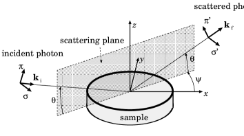
Figure 1: Geometry of the RXS experiment. Photon with polarization $\sigma$ or $\pi$ is scattered into the state of polarization $\sigma^{\prime}$ or $\pi^{\prime}$ at the Bragg angle $\theta$. The azimuthal angle $\psi$ describes the rotation of the sample around the scattering vector G.

II.2 Energy profiles

In localized models, the ground state and the intermediate state at each site are well specified by the eigenfunctions of the angular momentum operator, $|J,m\rangle$. The CEF and the intersite interaction usually lift the degeneracy in the ground state. Thus the ground state at site $j$ may be expressed as $|\psi_{0}\rangle_{j}=\sum_{m}c_{j}(m)|J,m\rangle$. On the other hand, in the intermediate state, we can neglect the CEF and the intersite interaction in a good approximation, since their energies are much smaller than the intra-atomic Coulomb interaction and the spin-orbit interaction (SOI) which give rise to the multiplet structure. Thus the intermediate state preserves the rotational symmetry. Under the assumption, as derived in Appendix, we obtain a general expression of the scattering amplitude at site $j$:

$$M_{j}(\mbox{\boldmath{$\epsilon$}}^{\prime},\mbox{\boldmath{$\epsilon$}},\omega) = \alpha_{0}(\omega)\mbox{\boldmath{$\epsilon$}}^{\prime}\cdot\mbox{\boldmath{$\epsilon$}}$$ (3)

$$- i\alpha_{1}(\omega)(\mbox{\boldmath{$\epsilon$}}^{\prime}\times\mbox{\boldmath{$\epsilon$}})\cdot\langle\psi_{0}|\textbf{J}|\psi_{0}\rangle$$

$$+ \alpha_{2}(\omega)\sum_{\nu}P_{\nu}(\mbox{\boldmath{$\epsilon$}}^{\prime},\mbox{\boldmath{$\epsilon$}})\langle\psi_{0}|z_{\nu}|\psi_{0}\rangle,$$

where

$$z_{1} \equiv Q_{x^{2}-y^{2}}=\frac{\sqrt{3}}{2}(J_{x}^{2}-J_{y}^{2}),$$ (4a)

$$z_{2} \equiv Q_{3z^{2}-r^{2}}=\frac{1}{2}(3J_{z}^{2}-J(J+1)),$$ (4b)

$$z_{3} \equiv Q_{yz}=\frac{\sqrt{3}}{2}(J_{y}J_{z}+J_{z}J_{y}),$$ (4c)

$$z_{4} \equiv Q_{zx}=\frac{\sqrt{3}}{2}(J_{z}J_{x}+J_{x}J_{z}),$$ (4d)

$$z_{5} \equiv Q_{xy}=\frac{\sqrt{3}}{2}(J_{x}J_{y}+J_{y}J_{x}),$$ (4e)

and

$$P_{1}(\mbox{\boldmath{$\epsilon$}}^{\prime},\mbox{\boldmath{$\epsilon$}}) = \frac{\sqrt{3}}{2}(\epsilon^{\prime}_{x}\epsilon_{x}-\epsilon^{\prime}_{y}\epsilon_{y}),$$ (5a)

$$P_{2}(\mbox{\boldmath{$\epsilon$}}^{\prime},\mbox{\boldmath{$\epsilon$}}) = \frac{1}{2}(2\epsilon^{\prime}_{z}\epsilon_{z}-\epsilon^{\prime}_{x}\epsilon_{x}-\epsilon^{\prime}_{y}\epsilon_{y}),$$ (5b)

$$P_{3}(\mbox{\boldmath{$\epsilon$}}^{\prime},\mbox{\boldmath{$\epsilon$}}) = \frac{\sqrt{3}}{2}(\epsilon^{\prime}_{y}\epsilon_{z}+\epsilon^{\prime}_{z}\epsilon_{y}),$$ (5c)

$$P_{4}(\mbox{\boldmath{$\epsilon$}}^{\prime},\mbox{\boldmath{$\epsilon$}}) = \frac{\sqrt{3}}{2}(\epsilon^{\prime}_{z}\epsilon_{x}+\epsilon^{\prime}_{x}\epsilon_{z}),$$ (5d)

$$P_{5}(\mbox{\boldmath{$\epsilon$}}^{\prime},\mbox{\boldmath{$\epsilon$}}) = \frac{\sqrt{3}}{2}(\epsilon^{\prime}_{x}\epsilon_{y}+\epsilon^{\prime}_{y}\epsilon_{x}).$$ (5e)

Here we have suppressed the dependence on $j$ in the right hand side of Eq. (3). The energy profiles are given by only three functions, $\alpha_{0}(\omega)$, $\alpha_{1}(\omega)$, and $\alpha_{2}(\omega)$, whose expressions are explicitly given in Appendix.

Several facts are immediately deduced from Eq. (3). First, since the scalar, dipole, and quadrupole terms exhaust the amplitude, the octupole ordering alone does not give rise to the RXS amplitude. Second, the choice of the CEF parameters in the ground state does not affect the shape of energy profiles $\alpha_{0}(\omega)$, $\alpha_{1}(\omega)$ and $\alpha_{2}(\omega)$, although it affects the expectation values of dipole and/or quadrupole operators. Third, $\alpha_{0}(\omega)$ has no contribution to the forbidden Bragg spots in the antiferro-type structure. In order to calculate the energy profiles, however, we need to know explicitly wavefunctions of the intermediate state, which are discussed in the next section.

II.3 Absorption coefficient

Within the $E1$ transition, the absorption coefficient is given by

$$A(\omega)\propto\sum_{j}\sum_{\alpha}\sum_{\Lambda}|\langle\Lambda|x_{\alpha,j}|\psi_{0}\rangle|^{2}\frac{\Gamma/\pi}{(\hbar\omega-E_{\Lambda}+E_{0})^{2}+\Gamma^{2}},$$ (6)

where $|\Lambda\rangle$ with energy $E_{\Lambda}$ represents the final state, which is equivalent to the intermediate state of RXS. A comparison of Eq. (6) with Eq. (2) leads to

$$A(\omega)\propto-{\rm Im}\,\alpha_{0}(\omega),$$ (7)

where Im $X$ denotes the imaginary part of $X$.

III RXS spectra from NpO₂

III.1 Quartet ground state

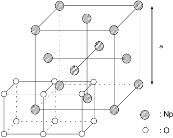
Figure 2: Crystal structure of NpO₂. Gray circles denote Np ions and open circles represent O ions.

NpO₂ has the CaF₂ type structure ($F_{m\overline{3}m}$) with a lattice constant $a=5.431$ Å at room temperature, as schematically shown in Fig. 2.Osborne and E. F. Westrum (1953) Np ions are tetravalent in NpO₂, as confirmed by the isomer shift in Mössbauer spectraDunlap et al. (1968) and by the neutron diffraction experiment.Delapalme et al. (1980) In a localized description, each Np ion is in the $(5f)^{3}$-configuration. The Hamiltonian of Np ions consists of the intra-atomic Coulomb interaction between $5f$ electrons in addition to the SOI of $5f$ electrons. The Slater integrals for the Coulomb interaction and the SOI parameters are evaluated within the Hatree-Fock approximation (HFA),Cowan (1981) and are listed in Table 1. Because the isotropic parts of the Coulomb interaction $F^{0}$’s are known to be well screened in solids compared to those of the anisotropic parts, the former quantities are multiplied by a factor 0.25 while the latter’s are by 0.8. Within the HFA, the ground state has the ten-fold degeneracy corresponding to $J=9/2$ multiplet. The choice of the multiplying factors does not alter this conclusion. Nagao and Igarashi (2003) Note that these states of $J=9/2$ are slightly deviated from those of the perfect Russell-Saunders (RS) coupling scheme with $L=6$ and $S=3/2$ due to the presence of the strong SOI. For instance, ${\textbf{L}}^{2}$ and ${\textbf{S}}^{2}$ take values 39.752 and 3.237 respectively, compared to the RS values 42 and 3.75.

Table 1: Slater integrals and spin-orbit interaction parameters in the $(3d)^{10}(5f)^{3}$ configuration within the HF approximation (in units of eV).Cowan (1981)

$F^{k}(3d,3d)$	$F^{k}(3d,5f)$	$F^{k}(5f,5f)$	$G^{k}(3d,5f)$
$F^{0}$    180.1		$F^{0}$    19.61
$F^{2}$    92.04		$F^{2}$    9.909
$F^{4}$    59.28		$F^{4}$    6.491
		$F^{6}$    4.769
$\zeta_{3d}=$ 76.254	$\zeta_{5f}=$ 0.298

In crystal, the ten-fold degeneracy is lifted by the CEF. Under the cubic symmetry, the CEF Hamiltonian $H_{\textrm{C}EF}$ may be expressed as

$$H_{\textrm{C}EF}=B_{4}(O_{4}^{0}+5O_{4}^{4})+B_{6}(O_{6}^{0}-21O_{6}^{4}),$$ (8)

where $O_{k}^{q}$’s represent Stevens operator equivalence. Thereby the degenerate levels are split into one doublet $\Gamma_{6}$ and two quartets $\Gamma_{8}^{(1)}$ and $\Gamma_{8}^{(2)}$. The level scheme has been analyzed by the inelastic neutron scattering, which yields an estimate of CEF parameters as $B_{4}=-3.03\times 10^{-2}$ meV and $B_{6}=2.36\times 10^{-4}$ meV. Amoretti et al. (1992) The lowest levels are given by the $\Gamma_{8}^{(2)}$, which is separated about 55 meV from another quartet $\Gamma_{8}^{(1)}$. Diagonalizing Eq. (8), we obtain the bases of the lowest quartet as

$$\left|+\uparrow\right\rangle = c_{1}\left|+\frac{9}{2}\right\rangle+c_{2}\left|+\frac{1}{2}\right\rangle+c_{3}\left|-\frac{7}{2}\right\rangle,$$ (9)

$$\left|+\downarrow\right\rangle = c_{1}\left|-\frac{9}{2}\right\rangle+c_{2}\left|-\frac{1}{2}\right\rangle+c_{3}\left|+\frac{7}{2}\right\rangle,$$ (10)

$$\left|-\uparrow\right\rangle = c_{4}\left|+\frac{5}{2}\right\rangle+c_{5}\left|-\frac{3}{2}\right\rangle,$$ (11)

$$\left|-\downarrow\right\rangle = c_{4}\left|-\frac{5}{2}\right\rangle+c_{5}\left|+\frac{3}{2}\right\rangle,$$ (12)

with $c_{1}=0.2757,c_{2}=-0.4483,c_{3}=0.8503,c_{4}=-0.9751$ and $c_{5}=0.2216$. State $|m\rangle$ denotes the eigenstate with $J_{z}=m$. Symbols $\tau$ ($=\pm$) and $\sigma$ ($=\uparrow,\downarrow$) are introduced to represent the state $|\tau,\sigma\rangle$, which distinguish non-Kramers’ and Kramers’ pairs, respectively.

III.2 Triple-k structure

The four-fold degeneracy in the ground $\Gamma_{8}^{(2)}$ quartet may be lifted by the intersite interaction, giving rise to induced multipole moments. Actually, several experiments tell us that the time-reversal symmetry is broken with nearly zero dipole moment in the ordered phase below $T_{0}=25.5$ K.Kopmann et al. (1998); Tokunaga et al. (2005) These observations lead Santini and Amoretti to propose the antiferro ordering of $T_{xyz}$-type ($T_{xyz}\equiv\frac{\sqrt{15}}{6}\overline{J_{x}J_{y}J_{z}}$). Santini and Amoretti (2000, 2002) Here the overline on operators means symmetrization, for example, $\overline{J_{x}J_{y}^{2}}=J_{x}J_{y}^{2}+J_{y}J_{x}J_{y}+J_{y}^{2}J_{x}$.Shiina et al. (1997). Unfortunately, this phase would not give rise to the RXS intensities observed in the experiments.

An important observation is that no external distortion from cubic structure exists in the ordered phase, that is, the unit cell remains cubic below $T_{0}$. This leads us to consider the triple-k ordering, since it allows the crystal to keep the cubic symmetry. As schematically shown in Fig. 3 (c), the triple-k structure is defined by all three members of the star of ${\textbf{k}}=\langle 001\rangle$ simultaneously present on each site of the lattice; there are four sublattices 1, 2, 3 and 4 at $(0,0,0),(\frac{1}{2},\frac{1}{2},0),(0,\frac{1}{2},\frac{1}{2})$ and $(\frac{1}{2},0,\frac{1}{2})$, respectively.

III.2.1 octupole ordering

We start by the octupole ordering of $\Gamma_{5u}$-type proposed by Paixão et al.Paixão et al. (2002) The corresponding octupole operators are defined by

$$T_{x}^{\beta} = \frac{\sqrt{15}}{6}\overline{J_{x}(J_{y}^{2}-J_{z}^{2})},$$ (13a)

$$T_{y}^{\beta} = \frac{\sqrt{15}}{6}\overline{J_{y}(J_{z}^{2}-J_{x}^{2})},$$ (13b)

$$T_{z}^{\beta} = \frac{\sqrt{15}}{6}\overline{J_{z}(J_{x}^{2}-J_{y}^{2})}.$$ (13c)

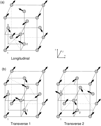
Figure 3: Triple-k antiferro arrangements. (a) a longitudinal pattern and (b) two transverse patterns (1 and 2). Arrows illustrate the direction of the multipole moment and number 1, 2, 3 and 4 specify the sublattices. Oxygen ions are omitted. Arrows indicate vector $(\langle J_{x}\rangle,\langle J_{y}\rangle,\langle J_{z}\rangle)$, $(\langle Q_{yz}\rangle,\langle Q_{zx}\rangle,\langle Q_{xy}\rangle)$, and $(\langle T^{\beta}_{x}\rangle,\langle T^{\beta}_{y}\rangle,\langle T^{\beta}_{z}\rangle)$, corresponding to the dipole, quadrupole, and octupole orderings, respectively.

Defining operators,

$$T_{p}=\left\{\begin{array}[]{lcl}\frac{1}{\sqrt{3}}\left(T_{x}^{\beta}+T_{y}^{\beta}+T_{z}^{\beta}\right)&{\textrm{f}or}&p=111,\\ \frac{1}{\sqrt{3}}\left(T_{x}^{\beta}-T_{y}^{\beta}-T_{z}^{\beta}\right)&{\textrm{f}or}&p=\overline{1}11,\\ \frac{1}{\sqrt{3}}\left(-T_{x}^{\beta}+T_{y}^{\beta}-T_{z}^{\beta}\right)&{\textrm{f}or}&p=1\overline{1}1,\\ \frac{1}{\sqrt{3}}\left(-T_{x}^{\beta}-T_{y}^{\beta}+T_{z}^{\beta}\right)&{\textrm{f}or}&p=11\overline{1},\\ \end{array}\right.$$ (14)

we assign them to each sublattice. Each $T_{p}$ operator has eigenvalues $\pm t_{1}$ ($t_{1}=-6.102$) and doubly degenerated $0$. The eigenstates of eigenvalues $\pm t_{1}$ are connected to each other by the time-reversal operation, and so are two degenerate states of eigenvalue 0. For example, the eigenstate of eigenvalue $-t_{1}$ for $T_{111}$ is explicitly written as

$$|-t_{1}\rangle = \frac{1}{2}{\textrm{e}}^{{\textrm{i}}\left(\theta_{111}-\frac{\pi}{2}\right)}\left[|+\uparrow\rangle+{\textrm{e}}^{-{\textrm{i}}\frac{\pi}{4}}|+\downarrow\rangle\right]$$ (15)

$$-\frac{1}{2}\left[|-\uparrow\rangle+{\textrm{e}}^{{\textrm{i}}\frac{3\pi}{4}}|-\downarrow\rangle\right],$$

with $\theta_{111}$ being an angle between vector $(1,1,1)$ and the $z$ axis, that is, $\cos\theta_{111}=\sqrt{1/3}$, $\sin\theta_{111}=\sqrt{2/3}$. This state is different from a ground state assumed by Lovesey et al, who considered the state deviating from $\Gamma_{8}$ quartet.Lovesey et al. (2003) Using the eigenstates as bases, $T_{p}$ is represented as

$$T_{p}=\left(\begin{array}[]{cccc}-t_{1}&0&0&0\\ 0&+t_{1}&0&0\\ 0&0&0&0\\ 0&0&0&0\\ \end{array}\right).$$ (16)

The ground state is given by assigning either of eigenstates of $\pm t_{1}$ to each sublattice; which eigenstate is relevant depends on the sign of acting mean field. As shown in Fig. 3, one longitudinal order and two transverse orders are possible in the triple-k ordering; for the longitudinal one, eigenstates of $T_{111}$, $T_{\overline{1}11}$, $T_{1\overline{1}1}$ and $T_{11\overline{1}}$ are assigned to sublattices 1, 3, 4 and 2, respectively; for two transverse orders, eigenstates of of $T_{111}$, $T_{\overline{1}11}$, $T_{1\overline{1}1}$, and $T_{11\overline{1}}$, are assigned to sublattices 1, 2, 3 and 4, and to 1, 4, 2 and 3, respectively.

Introducing the quadrupole operators,

$$Q_{p}=\left\{\begin{array}[]{lcl}\frac{1}{\sqrt{3}}\left(Q_{yz}+Q_{zx}+Q_{xy}\right)&{\textrm{f}or}&p=111,\\ \frac{1}{\sqrt{3}}\left(Q_{yz}-Q_{zx}-Q_{xy}\right)&{\textrm{f}or}&p=\overline{1}11,\\ \frac{1}{\sqrt{3}}\left(-Q_{yz}+Q_{zx}-Q_{xy}\right)&{\textrm{f}or}&p=1\overline{1}1,\\ \frac{1}{\sqrt{3}}\left(-Q_{yz}-Q_{zx}+Q_{xy}\right)&{\textrm{f}or}&p=11\overline{1},\\ \end{array}\right.$$ (17)

we can construct the quadrupole ordering state by assigning them to each sublattice in the same way as for octupole orderings. Since $Q_{p}$’s and $T_{p}$’s are simultaneously diagonalized because of commuting with each other, $Q_{p}$ could be represented as

$$Q_{p}=\left(\begin{array}[]{cccc}-q_{1}&0&0&0\\ 0&-q_{1}&0&0\\ 0&0&+q_{1}&0\\ 0&0&0&+q_{1}\\ \end{array}\right),$$ (18)

with $q_{1}=-8.273$.

Let the octupole ordering be primarily realized. Then, each Np ion is in the eigenstate of the eigenvalue $-t_{1}$ (or $t_{1}$). Since the state is also the eigenstate of the eigenvalue $-q_{1}$, the quadrupole ordering is simultaneously induced. On the other hand, if the quadrupole order is primary, each Np ion is in the eigenstate of the eigenvalue $-q_{1}$ or $q_{1}$. For the case of eigenvalue $-q_{1}$, two eigensates are to be degenerate and give eigenvalues $-t_{1}$ and $t_{1}$ to the octupole moment $T_{p}$, and thereby the net octupole moment becomes zero. For the case of $q_{1}$, two eigenstates are also to be degenerate and give the eigenvalue 0 to $T_{p}$. In either case, the quadrupole order carries no octupole order.

III.2.2 dipole ordering

Although the dipole ordering is ruled out in NpO₂, it may be interesting to discuss here what happens in the dipole ordering. Introducing the dipole operators,

$$J_{p}=\left\{\begin{array}[]{lcl}\frac{1}{\sqrt{3}}\left(J_{x}+J_{y}+J_{z}\right)&{\textrm{f}or}&p=111,\\ \frac{1}{\sqrt{3}}\left(J_{x}-J_{y}-J_{z}\right)&{\textrm{f}or}&p=\overline{1}11,\\ \frac{1}{\sqrt{3}}\left(-J_{x}+J_{y}-J_{z}\right)&{\textrm{f}or}&p=1\overline{1}1,\\ \frac{1}{\sqrt{3}}\left(-J_{x}-J_{y}+J_{z}\right)&{\textrm{f}or}&p=11\overline{1},\\ \end{array}\right.$$ (19)

we can construct the dipole ordering state by assigning them to each sublattice in the same way as in the octupole ordering. Note that $J_{p}$ and $Q_{p}$ are simultaneously diagonalized, because both operators commute with each other. Within the bases of simultaneous eigenstates of $J_{p}$ and $Q_{p}$, the relevant operators are represented as

$$J_{p} = \left(\begin{array}[]{cccc}-j_{1}&0&0&0\\ 0&+j_{1}&0&0\\ 0&0&-j_{2}&0\\ 0&0&0&+j_{2}\\ \end{array}\right),$$ (24)

$$Q_{p} = \left(\begin{array}[]{cccc}-q_{1}&0&0&0\\ 0&-q_{1}&0&0\\ 0&0&+q_{1}&0\\ 0&0&0&+q_{1}\\ \end{array}\right),$$ (29)

$$T_{p} = \left(\begin{array}[]{cccc}0&-t_{1}&0&0\\ -t_{1}&0&0&0\\ 0&0&0&0\\ 0&0&0&0\\ \end{array}\right),$$ (34)

where $j_{1}=3.27$, $j_{2}=0.18$ with parameters given in NpO₂. The magnetic moment is evaluated on either of eigenstates of $\pm j_{1}$: $\langle L_{p}+2S_{p}\rangle=2.48$ ($L_{p}$ and $S_{p}$ are defined as in the same way as $J_{p}$).

In the dipole ordering, the ground state is given by assigning one of the eigenstates of $J_{p}$’s to each sublattice. Since $j_{1}$ is much larger than $j_{2}$, the ground state is likely to be either of eigenstates of $\pm j_{1}$. It is obvious from Eqs. (29) and (34) that the dipole ordering induces the quadrupole moment but no octupole moment. Note that, if the quadrupole ordering is primary, no dipole moment is induced, because the doubly-degenerate eigenstates of $Q_{p}$ are the eigenstates of $\pm j_{1}$ of $J_{p}$.

III.3 RXS spectra

Irrespective of whether the octupole or quadrupole ordering is realized, RXS amplitudes are generated at each site, according to Eq. (3). They are proportional to $q_{1}\alpha_{2}(\omega)(P_{3}+P_{4}+P_{5})$ for the simultaneous eigenstate of $T_{111}$ and $Q_{111}$, to $q_{1}\alpha_{2}(\omega)(P_{3}-P_{4}-P_{5})$ for the simultaneous eigenstate of $T_{\overline{1}11}$ and $Q_{\overline{1}11}$, to $q_{1}\alpha_{2}(\omega)(-P_{3}+P_{4}-P_{5})$ for the simultaneous eigenstate of $T_{1\overline{1}1}$ and $Q_{1\overline{1}1}$, and to $q_{1}\alpha_{2}(\omega)(-P_{3}-P_{4}+P_{5})$ for the simultaneous eigenstate of $T_{11\overline{1}}$ and $Q_{11\overline{1}}$. On the scattering vector ${\textbf{G}}=(hh\ell)$ with $h+\ell=odd$, these amplitudes are summed up with a positive sign for sublattices 1 and 2 and with a negative sign for sublattices 3 and 4. Therefore, the total RXS amplitude becomes proportional to $q_{1}\alpha_{2}(\omega)P_{5}$ for the longitudinal order, while they are proportional to $q_{1}\alpha_{2}(\omega)P_{3}$ and $q_{1}\alpha_{2}(\omega)P_{4}$ for the two transverse orders. Note that a similar analysis is applied to the dipole ordering. In this case, both the dipole and quadrupole terms contribute to the amplitude. These results are summarized in Table 2. For the transverse case, our present treatment could be extended applying to the RXS spectra detected at Np $M_{4}$ edges in U_0.75Np₂O₂.Wilkins et al. (2004) In this compound, the spectra may be interpreted as a consequence brought about by the transverse type of triple-k AFO ordering driven by the same ordering pattern at U sites.

Polarization dependences become particularly simple for ${\textbf{G}}=(00\ell)$ ($\ell=$ odd) in the octupole and quadrupole orderings. They are explicitly written in the scattering geometry shown in Fig. 1 as $P_{3}=0$, $P_{4}=0$, $P_{5}=(\sqrt{3}/2)\sin 2\psi$ in the $\sigma-\sigma^{\prime}$ channel, while $P_{3}=(\sqrt{3}/2)\cos\theta\cos\psi$, $P_{4}=(\sqrt{3}/2)\cos\theta\sin\psi$, $P_{5}=(\sqrt{3}/2)\sin\theta\cos 2\psi$ in the $\sigma-\pi^{\prime}$ channel. Figure 4 shows the azimuthal-angle dependence of the spectra ${\textbf{G}}=(003)$ in comparison with the experiment. Paixão et al. (2002); Caciuffo et al. (2003) The experimental data are well fitted by $\sin^{2}2\psi$ in the $\sigma$-$\sigma^{\prime}$ channel, and $\sin^{2}\theta\cos^{2}2\psi$ in the $\sigma$-$\pi^{\prime}$ channel. The two transverse orders cannot reproduce the experimental curves, as seen from panel (b). Paixão et al. and Caciuffo et al. analyzed their experimental data and concluded that the longitudinal order gives rise to this dependence.Paixão et al. (2002); Caciuffo et al. (2003) The present analysis confirms their result. Note that, based on a group theoretical point of view, Nikolaev and Michel have obtained the same result.Nikolaev and Michel (2003)

Table 2: RXS amplitudes in triple-k ordering, for ${\bf G}=(hh\ell)$ with $h+\ell=odd$.

		RXS amplitude
	Longitudinal	Transverse 1	Transverse 2
dipole	-${\rm i}\alpha_{1}(\omega)\langle\psi_{0}|J_{z}|\psi_{0}\rangle(\mbox{\boldmath{$\epsilon$}}^{\prime}\times\mbox{\boldmath{$\epsilon$}})_{z}$	-${\rm i}\alpha_{1}(\omega)\langle\psi_{0}|J_{x}|\psi_{0}\rangle(\mbox{\boldmath{$\epsilon$}}^{\prime}\times\mbox{\boldmath{$\epsilon$}})_{x}$	-${\rm i}\alpha_{1}(\omega)\langle\psi_{0}|J_{y}|\psi_{0}\rangle(\mbox{\boldmath{$\epsilon$}}^{\prime}\times\mbox{\boldmath{$\epsilon$}})_{y}$
	$+\alpha_{2}(\omega)\langle\psi_{0}|Q_{5}|\psi_{0}\rangle P_{5}(\mbox{\boldmath{$\epsilon$}}^{\prime},\mbox{\boldmath{$\epsilon$}})$	$+\alpha_{2}(\omega)\langle\psi_{0}|Q_{3}|\psi_{0}\rangle P_{3}(\mbox{\boldmath{$\epsilon$}}^{\prime},\mbox{\boldmath{$\epsilon$}})$	$+\alpha_{2}(\omega)\langle\psi_{0}|Q_{4}|\psi_{0}\rangle P_{4}(\mbox{\boldmath{$\epsilon$}}^{\prime},\mbox{\boldmath{$\epsilon$}})$
quadrupole	$\alpha_{2}(\omega)\langle\psi_{0}|Q_{5}|\psi_{0}\rangle P_{5}(\mbox{\boldmath{$\epsilon$}}^{\prime},\mbox{\boldmath{$\epsilon$}})$	$\alpha_{2}(\omega)\langle\psi_{0}|Q_{3}|\psi_{0}\rangle P_{3}(\mbox{\boldmath{$\epsilon$}}^{\prime},\mbox{\boldmath{$\epsilon$}})$	$\alpha_{2}(\omega)\langle\psi_{0}|Q_{4}|\psi_{0}\rangle P_{4}(\mbox{\boldmath{$\epsilon$}}^{\prime},\mbox{\boldmath{$\epsilon$}})$
octupole	$\alpha_{2}(\omega)\langle\psi_{0}|Q_{5}|\psi_{0}\rangle P_{5}(\mbox{\boldmath{$\epsilon$}}^{\prime},\mbox{\boldmath{$\epsilon$}})$	$\alpha_{2}(\omega)\langle\psi_{0}|Q_{3}|\psi_{0}\rangle P_{3}(\mbox{\boldmath{$\epsilon$}}^{\prime},\mbox{\boldmath{$\epsilon$}})$	$\alpha_{2}(\omega)\langle\psi_{0}|Q_{4}|\psi_{0}\rangle P_{4}(\mbox{\boldmath{$\epsilon$}}^{\prime},\mbox{\boldmath{$\epsilon$}})$

Figure 4: Azimuthal-angle dependence of the RXS spectra from the triple-k AFO phases with ${\textbf{G}}=(003)$. (a) Longitudinal ordering. The open circles and filled triangles are experimental data, and the solid and broken lines are the calculated results, in the $\sigma$-$\sigma^{\prime}$ and $\sigma$-$\pi^{\prime}$ channels, respectively.Caciuffo et al. (2003) (b) Transverse orderings in the $\sigma$-$\pi^{\prime}$ channel. No RXS signal is expected from these orders in the $\sigma$-$\sigma^{\prime}$ channel. The solid and broken lines are the calculated results for the two transverse orders.

Now we discuss the energy profiles. In order to calculate them, we need the wavefunctions in the intermediate state. We first evaluate the Slater integrals for the Coulomb interaction and the SOI parameters within the HFA, which are shown in Table 3. These values are reduced by taking account of screening effects. The reduction factors are set the same as in the ground state. The Hamiltonian of the intermediate state, consisting of the full intra-atomic Coulomb interactions between $5f$-$5f$, $5f$-$3d$ and $3d$-$3d$ electrons as well as the SOI of $5f$ and $3d$ electrons, is represented by $1001\times(2j_{d}+1)$ microscopic states with the total angular momentum of the core hole $j_{d}=3/2$ and $5/2$ corresponding to the $M_{4}$ and the $M_{5}$ edges, respectively. Diagonalizing the Hamiltonian matrix, we obtain multiplet structures in the intermediate state. The $\alpha_{2}(\omega)$ is calculated by using Eq. (A.8).

Table 3: Slater integrals and spin-orbit interaction parameters in the $(3d)^{9}(5f)^{4}$ configuration within the HFA (in units of eV).Cowan (1981)

$F^{0}$    181.0	$F^{0}$    29.13	$F^{0}$    20.54	$G^{1}$    2.158
$F^{2}$    92.62	$F^{2}$    2.749	$F^{2}$    10.39	$G^{3}$    1.306
$F^{4}$    59.67	$F^{4}$    1.281	$F^{4}$    6.943	$G^{5}$    0.914
		$F^{6}$    5.017
$\zeta_{3d}=$ 77.278	$\zeta_{5f}=$ 0.339

The energy profile is proportional to $|\alpha_{2}(\omega)|^{2}$ in the octupole ordering phase. The calculated spectra around $M_{4}$ and $M_{5}$ edges are displayed with several choices of $\Gamma$ values in Fig. 5. The origin of the energy is adjusted such that the peak of the RXS spectrum is located at the experimental peak position. Since there is no reliable estimation for the $\Gamma$ value, we choose three typical values $\Gamma=0.01,0.5$ and $2.0$ eV. The spike-like curves with $\Gamma=0.01$ eV directly reflect the multiplet splittings of the intermediate states. For the $M_{4}$ edge, the choice $\Gamma=0.5$ eV makes a multi-peak-structure line-shape. It merges into a single-peak structure around $\Gamma\simeq 1.0$ eV. The choice $\Gamma=2.0$ eV corresponds to one of better fittings with the experimental line shape.Paixão et al. (2002); Caciuffo et al. (2003) The core-level energy is adjusted such that the calculated peak at the $M_{4}$ edge with $\Gamma=2$ eV coincides with the experimental one. Paixao et al. reported that the line shape is well fitted by a Lorentzian-squared rather than a Lorentzian one.Paixão et al. (2002) As shown above, the line shape is basically determined by the multiplet structure, which is smeared by the life-time broadening. Whether it looks Lorentzian-squared or Lorentzian seems unimportant. As for the spectra at the $M_{5}$ edge, their shape depends rather sensitively on the value of $\Gamma$ compared to that at the $M_{4}$ edge.

Figure 5: Energy profiles $|\alpha_{2}(\omega)|^{2}$ at the Np $M_{4}$ (right panels) and $M_{5}$ (left panels) edges. The lines represent the calculated results for $\Gamma=0.01,0.5$ and $2.0$ eV, respectively, from bottom to top panels. In the top right panel, The open circles and crosses are experimental data in NpO₂.Paixão et al. (2002); Caciuffo et al. (2003) The peak heights of them are adjusted to that of the calculated value.

The energy profile in the dipole ordering is given by the sum of the dipole and quadrupole terms. However, $|\alpha_{1}(\omega)|^{2}$ is about two orders of magnitude larger than $|\alpha_{2}(\omega)|^{2}$. For instance, $|\alpha_{1}(\omega)|^{2}\sim 192\times|\alpha_{2}(\omega)|^{2}$ when $\Gamma=2.0$ eV. Thus the dipole term usually dominates the quadrupole term. Although the dipole ordering is ruled out from experiments, we show $|\alpha_{1}(\omega)|^{2}$ in Fig. 6 as a reference. The peak at the $M_{4}$ edge with $\Gamma=2$ eV is at 3847.5 eV, 0.7 eV higher than the peak position of $|\alpha_{2}(\omega)|^{2}$. Note that the spectral shape at the $M_{5}$ edge depends on $\Gamma$ more sensitive than that at the $M_{4}$ edge.

Figure 6: Energy profiles $|\alpha_{1}(\omega)|^{2}$ at the Np $M_{4}$ (right panels) and $M_{5}$ (left panels) edges. The lines represent the calculated results for $\Gamma=0.01,0.5$ and $2.0$ eV, respectively, from bottom to top panels.

III.4 Absorption coefficient

The absorption coefficient is proportional to $-{\rm Im}\ \alpha_{0}(\omega)$. We calculate $\alpha_{0}(\omega)$ from Eq. (A.4) in the same way as in the calculation of $\alpha_{1}(\omega)$ and $\alpha_{2}(\omega)$. The calculated results are shown in Fig. 7 at the $M_{4}$ and $M_{5}$ edges. The present calculation confirms the previous multiplet calculation by Lovesey et al., in which $-\textrm{Im}\ \alpha_{0}(\omega)$ has been calculated at the $M_{\textrm{4}}$ edge for $\Gamma=0.7$ eV.Lovesey et al. (2003) With increasing values of $\Gamma$, the multiplet structure merges into a single peak. The peak position at the $M_{4}$ edge with $\Gamma=2$ eV is about $0.35$ eV higher than that in $|\alpha_{2}(\omega)|^{2}$.

Figure 7: Absorption coefficients as functions of the photon energy at the Np $M_{4}$ (right panel) and $M_{5}$ (left panel) edges. The bold solid and dotted lines represent the calculated results for $\Gamma=0.5$ and $2.0$ eV, respectively. The vertical bars represent $\delta$-functions with $\Gamma=0$.

IV Concluding remarks

In this paper, we have studied the RXS spectra at the Np M_4,5 edges in the triple-k multipole ordering phase of NpO₂, on the basis of a localized electron model. We have derived an expression of scattering amplitudes in the $E$1 process, assuming that the rotational invariance is preserved in the intermediate states of the scattering process. This is a reasonable assumption when the multiplet energy is larger than those of the CEF and the intersite interaction. On the basis of this expression, we have analyzed the RXS spectra in NpO₂. Assuming the $\Gamma_{8}$-quartet ground state, we have constructed the triple-k ordering ground state. The energy profiles have been calculated by taking full account of the multiplet structure in the intermediate state, in agreement with the experiment.

RXS signals on multipole ordering superlattice spots have also been observed and analyzed at L_2,3 edges of rare-earth metals in their compounds such as CeB₆ and DyB₂C₂.Nakao et al. (2001); Yakhou et al. (2001); Tanaka et al. (1999); Hirota et al. (2000); Matsumura et al. (2005); Nagao and Igarashi (2001); Igarashi and Nagao (2002, 2003) The intermediate state is created by the transition from the $2p$-core to $5d$ states. Since the $5d$ states are considerably delocalized with forming energy bands, the assumption that the intermediate state preserves the rotational invariance becomes less accurate. An extension of the formula is left in future study.

Appendix A Derivation of Eq. (3)

We derive a general expression of RXS amplitude under the assumption that the intermediate state keeps the rotational symmetry at each site. The following derivation emphasizes the multiplet structure in the intermediate state. Thereby it is more general than the previous analyses, in which the fast collision approximation was adopted by replacing the multiplets with a single level.Hannon et al. (1989); Luo et al. (1993); Lovesey and Balcar (1996) A part of the results found in this Appendix were used in Ref. Nagao and Igarashi, 2005 when we analyzed the RXS spectra form URu₂Si₂.

Let the core hole be created at site $j$ in the intermediate state. We express the intermediate state as $|\Lambda\rangle=|J^{\prime},M,i\rangle$, where the magnitude $J^{\prime}$ and the magnetic quantum number $M$ of total angular momentum (including a core-hole angular momentum) are good quantum numbers. To distinguish multiplets having the same $J^{\prime}$ value but having the different energy, we introduce the index $i$. Defining $M_{\alpha\alpha^{\prime}}$ by $M_{j}(\mbox{\boldmath{$\epsilon$}}^{\prime},\mbox{\boldmath{$\epsilon$}},\omega)=\sum_{\alpha\alpha^{\prime}}\epsilon^{\prime}_{\alpha}\epsilon_{\alpha^{\prime}}M_{\alpha\alpha^{\prime}}(j,\omega)$, we rewrite Eq. (2) as

$$M_{\alpha\alpha^{\prime}}(j,\omega) = \sum_{J^{\prime},M,i}E_{i}(\omega,J^{\prime})\langle\psi_{0}|x_{\alpha,j}|J^{\prime},M,i\rangle$$ (35)

$$\times\langle J^{\prime},M,i|x_{\alpha^{\prime},j}|\psi_{0}\rangle,$$

with

$$E_{i}(\omega,J^{\prime})=\frac{1}{\hbar\omega-(E_{J^{\prime},i}-E_{0})+i\Gamma}.$$ (36)

Assuming that the ground-state wavefunction is expressed as a linear combination of $|J,m\rangle$ at each site,

$$|\psi_{0}\rangle=\sum_{m}c_{j}(m)|J,m\rangle,$$ (37)

and inserting this equation into Eq. (35), we obtain

$${M}_{\alpha\alpha^{\prime}}(j,\omega)=\sum_{m,m^{\prime}}c^{\ast}_{j}(m)c_{j}(m^{\prime}){M}_{\alpha\alpha^{\prime}}^{m,m^{\prime}}(\omega),,$$ (38)

with

$${M}_{\alpha\alpha^{\prime}}^{m,m^{\prime}}(\omega) = \sum_{J^{\prime}}\sum_{i=1}^{N_{J^{\prime}}}E_{i}(\omega,J^{\prime})\sum_{M=-J^{\prime}}^{J^{\prime}}$$ (39)

$$\times\langle J,m|x_{\alpha}|J^{\prime},M,i\rangle\langle J^{\prime},M,i|x_{\alpha^{\prime}}|J,m^{\prime}\rangle,$$

where the number of the multiplets having the value $J$ is denoted by $N_{J}$. We have suppressed the index $j$ specifying the core-hole site. The selection rule for the $E$1 process confines the range of the summation over $J^{\prime}$ to $J^{\prime}=J,J\pm 1$. The matrix element of the type $\langle J,m|x_{\alpha}|J^{\prime},M\rangle$ is analyzed by utilizing the Wigner-Eckart theorem for a vector operator with the use of the Wigner’s $3j$ symbol;Tinkham (1964)

$$\langle J,m|s_{\mu}|J^{\prime}M\rangle=(-1)^{J^{\prime}+m-1}\left(\begin{array}[]{ccc}J^{\prime}&1&J\\ M&\mu&-m\end{array}\right)(J||V_{1}||J^{\prime})$$ (40)

with $s_{\pm 1}=\mp(1/\sqrt{2})(x\pm iy)$, $s_{0}=z$. The symbol $(J||V_{1}||J^{\prime})$ denotes the reduced matrix element of the set of irreducible tensor operator of the first rank. Because of the nature of the dipole operators, ${M}^{m,m^{\prime}}(\omega)\neq{\textbf{0}}$ only when $|m-m^{\prime}|\leq 2$. After lengthy calculation, we obtain

$$M^{m,m}_{\alpha,\alpha^{\prime}}(\omega) = \left[\frac{1}{3}J(J+1)-m^{2}\right]\alpha_{2}(\omega)M^{3z^{2}-r^{2}}_{\alpha,\alpha^{\prime}}$$ (41a)

$$- {\textrm{i}}m\alpha_{1}(\omega)M^{z}_{\alpha,\alpha^{\prime}}+\alpha_{0}(\omega)\delta_{\alpha,\alpha^{\prime}},$$

$$M^{m,m+1}_{\alpha,\alpha^{\prime}}(\omega) = \frac{1}{2}f_{m}(2m+1)\alpha_{2}(\omega)(M^{zx}+{\textrm{i}}M^{yz})_{\alpha,\alpha^{\prime}}$$ (41b)

$$- {\textrm{i}}\frac{1}{2}f_{m}\alpha_{1}(\omega)(M^{x}+{\textrm{i}}M^{y})_{\alpha,\alpha^{\prime}},$$

$$M^{m+1,m}_{\alpha,\alpha^{\prime}}(\omega) = \frac{1}{2}f_{m}(2m+1)\alpha_{2}(\omega)(M^{zx}-{\textrm{i}}M^{yz})_{\alpha,\alpha^{\prime}}$$ (41c)

$$- {\textrm{i}}\frac{1}{2}f_{m}\alpha_{1}(\omega)(M^{x}-{\textrm{i}}M^{y})_{\alpha,\alpha^{\prime}},$$

$$M^{m,m+2}_{\alpha,\alpha^{\prime}}(\omega) = a_{m}^{\prime\prime}\alpha_{2}(\omega)(M^{x^{2}-y^{2}}+{\textrm{i}}M^{xy})_{\alpha,\alpha^{\prime}},$$ (41d)

$$M^{m+2,m}_{\alpha,\alpha^{\prime}}(\omega) = a_{m}^{\prime\prime}\alpha_{2}(\omega)(M^{x^{2}-y^{2}}-{\textrm{i}}M^{xy})_{\alpha,\alpha^{\prime}},$$ (41e)

where

$$f_{m} = \sqrt{(J-m)(J+m+1)},$$ (42)

$$a_{m}^{\prime\prime} = \frac{1}{2}f_{m}f_{m+1},$$ (43)

and the $3\times 3$ matrices, $M^{x}$, $M^{y}$, $M^{z}$, $M^{xy}$, $M^{yz}$, $M^{zx}$, $M^{x^{2}-y^{2}}$, and $M^{3z^{2}-r^{2}}$ are tabulated in Table 4.

Table 4: Antisymmetric matrices, $M^{x}$, $M^{y}$, $M^{z}$, and symmetric matrices $M^{yz}$, $M^{zx}$, $M^{xy}$, $M^{3z^{2}-r^{2}}$, $M^{x^{2}-y^{2}}$.

Antisymmetric	$M^{x}$	$M^{y}$	$M^{z}$
	$\left(\begin{array}[]{ccc}0&0&0\\ 0&0&1\\ 0&-1&0\\ \end{array}\right)$	$\left(\begin{array}[]{ccc}0&0&-1\\ 0&0&0\\ 1&0&0\\ \end{array}\right)$	$\left(\begin{array}[]{ccc}0&1&0\\ -1&0&0\\ 0&0&0\\ \end{array}\right)$
Symmetric	$M^{yz}$	$M^{zx}$	$M^{xy}$
	$\left(\begin{array}[]{ccc}0&0&0\\ 0&0&1\\ 0&1&0\\ \end{array}\right)$	$\left(\begin{array}[]{ccc}0&0&1\\ 0&0&0\\ 1&0&0\\ \end{array}\right)$	$\left(\begin{array}[]{ccc}0&1&0\\ 1&0&0\\ 0&0&0\\ \end{array}\right)$
	$M^{3z^{2}-r^{2}}$	$M^{x^{2}-y^{2}}$
	$\left(\begin{array}[]{ccc}-1&0&0\\ 0&-1&0\\ 0&0&2\\ \end{array}\right)$	$\left(\begin{array}[]{ccc}1&0&0\\ 0&-1&0\\ 0&0&0\\ \end{array}\right)$

The energy profiles are given by

$$\alpha_{0}(\omega) = \frac{2}{3}J(2J-1)F_{J-1}(\omega)+\frac{2}{3}J(J+1)F_{J}(\omega)$$ (44a)

$$+ \frac{2}{3}(2J^{2}+5J+3)F_{J+1}(\omega),$$

$$\alpha_{1}(\omega) = -(2J-1)F_{J-1}(\omega)-F_{J}(\omega)$$ (44b)

$$+ (2J+3)F_{J+1}(\omega),$$

$$\alpha_{2}(\omega) = \frac{4}{3}\left[-F_{J-1}(\omega)+F_{J}(\omega)-F_{J+1}(\omega)\right],$$ (44c)

with

$$F_{J^{\prime}}(\omega)=(-)^{J-J^{\prime}}|(J||V_{1}||J^{\prime})|^{2}\sum_{i=1}^{N_{J^{\prime}}}E_{i}(\omega,J^{\prime}).$$ (45)

Substituting Eqs. (41) into Eq. (38), we obtain the final expression Eq. (3).

References

• Murakami et al. (1998) Y. Murakami, J. P. Hill, D. Gibbs, M. Blume, I. Koyama, M. Tanaka, H. Kawata, T. Arima, Y. Tokura, K. Hirota, et al., Phys. Rev. Lett. 81, 582 (1998).
• Ishihara and Maekawa (1998) S. Ishihara and S. Maekawa, Phys. Rev. Lett. 80, 3799 (1998).
• Elfimov et al. (1999) I. S. Elfimov, V. I. Anisimov, and G. A. Sawatzky, Phys. Rev. Lett. 82, 4264 (1999).
• Benfatto et al. (1999) M. Benfatto, Y. Joly, and C. R. Natoli, Phys. Rev. Lett. 83, 636 (1999).
• Takahashi et al. (1999) M. Takahashi, J. Igarashi, and P. Fulde, J. Phys. Soc. Jpn. 68, 2530 (1999).
• Isaacs et al. (1990) E. D. Isaacs, D. B. McWhan, R. N. Kleiman, D. J. Bishop, G. E. Ice, P. Zschack, B. D. Gaulin, T. E. Mason, J. D. Garrett, and W. J. L. Buyers, Phys. Rev. Lett. 65, 3185 (1990).
• Mannix et al. (1999) D. Mannix, G. H. Lander, J. Rebizant, R. Caciuffo, N. Bernhoeft, E. Lidström, and C. Vettier, Phys. Rev. B 60, 15187 (1999).
• Longfield et al. (2002) M. J. Longfield, J. A. Paixão, N. Bernhoeft, G. H. Lander, F. Wastin, and J. Rebizant, Phys. Rev. B 66, 134421 (2002).
• Hannon et al. (1989) J. P. Hannon, G. T. Trammell, M. Blume, and D. Gibbs, Phys. Rev. Lett. 61, 1245 (1988); ibid. 62, 2644(E) (1989).
• Osborne and E. F. Westrum (1953) D. W. Osborne and J. E. F. Westrum, J. Chem. Phys. 21, 1884 (1953).
• Erdös et al. (1980) P. Erdös, G. Solt, Z. Żołnierek, A. Blaise, and J. M. Fournier, Physica 102B, 164 (1980).
• Dunlap et al. (1968) B. D. Dunlap, G. M. Kalvius, D. J. Lam, and B. Brodsky, J. Phys. Chem. Solids 29, 1365 (1968).
• Friedt et al. (1985) J. M. Friedt, F. J. Litterst, and J. Rebizant, Phys. Rev. B 32, 257 (1985).
• Cox and Frazer (1967) D. E. Cox and B. Frazer, J. Phys. Chem. Solids 28, 1649 (1967).
• Heaton et al. (1967) L. Heaton, M. H. Mueller, and J. M. Williams, J. Phys. Chem. Solids 28, 1651 (1967).
• Ross and Lam (1967) J. W. Ross and D. J. Lam, J. Appl. Phys. 38, 1451 (1967).
• Kopmann et al. (1998) W. Kopmann, F. J. Litterst, H. H. Klauß, M. Hillberg, W. Wagener, G. M. Kalvius, E. Schreier, F. J. Burghart, J. Rebizant, and G. H. Lander, J. Alloys Compd. 271-273, 463 (1998).
• Santini and Amoretti (2000) P. Santini and G. Amoretti, Phys. Rev. Lett. 85, 2188, 5481(E) (2000).
• Santini and Amoretti (2002) P. Santini and G. Amoretti, J. Phys. Soc. Jpn. Suppl. 71, 11 (2002).
• Paixão et al. (2002) J. A. Paixão, C. Detlefs, M. J. Longfield, R. Caciuffo, P. Santini, N. Bernhoeft, J. Rebizant, and G. H. Lander, Phys. Rev. Lett. 89, 187202 (2002).
• Tokunaga et al. (2005) Y. Tokunaga, Y. Homma, S. Kambe, D. Aoki, H. Sakai, E. Yamamoto, A. Nakamura, Y. Shiokawa, R. E. Walstedt, and H. Yasuoka, Phys. Rev. Lett. 94, 137209 (2005).
• Kiss and Fazekas (2003) A. Kiss and P. Fazekas, Phys. Rev. B 68, 174425 (2003).
• Kubo and Hotta (2005) K. Kubo and T. Hotta, Phys. Rev. B 71, 140404(R) (2005).
• Caciuffo et al. (2003) R. Caciuffo, J. A. Paixão, M. J. Longfield, P. Santini, N. Bernhoeft, and G. H. Lander, J. Phys.: Condens. Matter 15, S2287 (2003).
• Blume (1985) M. Blume, J. Appl. Phys. 57, 3615 (1985).
• Blume and Gibbs (1988) M. Blume and D. Gibbs, Phys. Rev. B 37, 1779 (1988).
• Hill and McMorrow (1996) J. P. Hill and D. F. McMorrow, Acta Cryst. A 52, 236 (1996).
• Delapalme et al. (1980) A. Delapalme, M. Forte, J. M. Fournier, J. Rebizant, and J. C. Spirlet, Physica 102B, 171 (1980).
• Cowan (1981) R. Cowan, The Theory of Atomic Structure and Spectra (University of California Press, Berkeley, 1981).
• Nagao and Igarashi (2003) T. Nagao and J. Igarashi, J. Phys. Soc. Jpn. 72, 2381 (2003).
• Amoretti et al. (1992) G. Amoretti, A. Blaise, R. Caciuffo, D. Cola, J. M. Fournier, M. T. Hutchings, G. H. Lander, R. Osborn, A. Severing, and A. D. Taylor, J. Phys.: Condens. Matter 4, 3459 (1992).
• Shiina et al. (1997) R. Shiina, H. Shiba, and P. Thalmeier, J. Phys. Soc. Jpn. 66, 1741 (1997).
• Lovesey et al. (2003) S. W. Lovesey, E. Balcar, C. Deltefs, G. van der Laan, D. S. Sivia, and U. Staub, J. Phys.: Condens. Matter 15, 4511 (2003).
• Wilkins et al. (2004) S. B. Wilkins, J. A. Paixão, R. Caciuffo, P. Javorsky, F. Wastin, J. Rebizant, C. Detlefs, N. Bernhoeft, P. Santini, and G. H. Lander, Phys. Rev. B 70, 214402 (2004).
• Nikolaev and Michel (2003) A. V. Nikolaev and K. H. Michel, Phys. Rev. B 68, 054112 (2003).
• Nakao et al. (2001) H. Nakao, K. Magishi, Y. Wakabayashi, Y. Murakami, K. Koyama, K. Hirota, Y. Endoh, and S. Kunii, J. Phys. Soc. Jpn. 70, 1857 (2001).
• Yakhou et al. (2001) F. Yakhou, V. Plakhty, H. Suzuki, S. Gavrilov, P. Burlet, L. Paolasini, C. Vettier, and S. Kunii, Phys. Lett. A 285, 191 (2001).
• Tanaka et al. (1999) Y. Tanaka, T. Inami, T. Nakamura, H. Yamauchi, H. Onodera, K. Ohyama, and Y. Yamaguchi, J. Phys.: Condens. Matter 11, L505 (1999).
• Hirota et al. (2000) K. Hirota, N. Oumi, T. Matsumura, H. Nakao, Y. Wakabayashi, Y. Murakami, and Y. Endoh, Phys. Rev. Lett. 84, 2706 (2000).
• Matsumura et al. (2005) T. Matsumura, D. Okuyama, N. Oumi, K. Hirota, H. Nakao, Y. Murakami, and Y. Wakabayashi, J. Phys. Soc. Jpn. 74, 1500 (2005).
• Nagao and Igarashi (2001) T. Nagao and J. Igarashi, J. Phys. Soc. Jpn. 70, 2892 (2001).
• Igarashi and Nagao (2002) J. Igarashi and T. Nagao, J. Phys. Soc. Jpn. 71, 1771 (2002).
• Igarashi and Nagao (2003) J. Igarashi and T. Nagao, J. Phys. Soc. Jpn. 72, 1279 (2003).
• Lovesey and Balcar (1996) S. W. Lovesey and E. Balcar, J. Phys.: Condens. Matter 8, 10983 (1996).
• Luo et al. (1993) J. Luo, G. T. Trammell, and J. P. Hannon, Phys. Rev. Lett. 71, 287 (1993).
• Nagao and Igarashi (2005) T. Nagao and J. Igarashi, J. Phys. Soc. Jpn. 74, 765 (2005).
• Tinkham (1964) M. Tinkham, Group Theory and Quantum Mechanics (McGraw-Hill, New York, 1964).