Gutzwiller study of spin-1 bosons in an optical lattice under a magnetic field

Abstract

We study spin-1 bosons in an optical lattice under a magnetic field by the Gutzwiller approximation. Our results thus obtained join the discontinuous phase boundary curves obtained by perturbative studies through a first-order transition. On the phase boundary curve, we also find a peculiar cusp structure originating from the degeneracy between different spin Mott states under a magnetic field. The magnetic field dependence of both fluctuation in the total number of bosons and the spin magnetization clarifies that the superfluid phase is divided into two regions reflecting the coexisting first- and second-order superfluid transitions.

Superfluid (SF) and Mott insulators (MI) are very interesting subjects in condensed matter physics. Recently, the transition between the SF and MI of spinless Bose atoms has been experimentally demonstrated in an optical lattice system Greiner closely following the theoretical proposal based on a Bose-Hubbard model (BHM) Fisher ; BHM due to Jaksch et al. Jaksch . In contrast to the case of fermions Review , the Gutzwiller approximation (GA) BoseGutz describes an accurate second-order SF-MI transition of spinless bosons, which is supported by quantum Monte Carlo simulations QMC .

Trapped spinor bosons have also been investigated both theoretically spintheory and experimentally spinorexp . In an optical lattice, MIDemlerZhou ; nematic1 and SFDemlerZhou ; Cheng phases of spinor bosons have been studied. MI phases under a magnetic field have also been studied recently magMI . The SF-MI transition in a spin-1 BHM has also been studied by a perturbative mean-field approximation (PMFA) Oosten , which treats the hopping process between adjacent sites as a perturbation Tsuchiya , by the GA Kimura , by a conventional mean-field approximation (CMFA) Krutitsky , and by density-matrix renormalization group in one dimension Rizzi . The GA and CMFA results show a possible first-order transition (FOT) at a part of the phase boundary curve, where the critical value of hopping matrix element just on the phase boundary is smaller than that obtained by the PMFA, which describes a second-order transition (SOT). On the other hand, the results obtained by the PMFA can also be obtained by the GA, which assumes a partial set of the full wave functions Kimura . Hence, generally speaking, the results obtained by the GA improve those obtained by the PMFA.

The PMFA approach has also been applied to the SF-MI transition in the spin-1 BHM under a magnetic field Uesugi ; Svidzinsky . However, the phase boundary curve obtained by the PMFA in the limit of a weak magnetic field ($B\rightarrow 0$) Uesugi ; Svidzinsky does not agree with that obtained by initially assuming zero magnetic field ($B=0$) Tsuchiya when the MI phase has an odd number of bosons. Moreover, the phase boundary obtained by the PMFA Uesugi ; Svidzinsky is a discontinuous function of magnetic field. These features might be attributed to the PMFA itself.

In this paper, we study the spin-1 BHM by the GA. In contrast to the PMFA, the GA shows that the SF-MI phase boundary is a continuous function of magnetic field even around a zero magnetic field. In the phase diagram, we also find a special point where a degeneracy of MI states with different spins plays an important role. We also investigate superfluid properties in terms of magnetization and fluctuation in the total number of bosons (FTNB) in the system. Both quantities, which are experimentally observable, have interesting magnetic field dependence originating from the coexisting FOT and SOT in the present system.

The BHM of spin-1 bosons DemlerZhou ; Tsuchiya ; Kimura ; nematic1 ; Uesugi ; Svidzinsky is given by $H=H_{\mathrm{h}op}+H_{\mathrm{i}nt}+H_{\rm mag}$ in standard notation Tsuchiya

$$H_{\mathrm{h}op} = -t\sum_{\langle i,j\rangle}\sum_{\alpha=0,\pm 1}({\hat{a}}_{i\alpha}^{\dagger}{\hat{a}}_{j\alpha}+{\hat{a}}_{j\alpha}^{\dagger}{\hat{a}}_{i\alpha}),$$

$$H_{\mathrm{i}nt} = \sum_{i}\big{[}-\mu{n}_{i}+\frac{U_{0}}{2}{n}_{i}({n}_{i}-1)+\frac{U_{2}}{2}({\mathbf{S}}_{i}^{2}-2n_{i})\big{]},$$

$$H_{\mathrm{m}ag} =- g\mu_{B}B\sum_{i}{S_{zi}}\equiv-b\sum_{i}{S_{zi}}.$$ (1)

Here, for simplicity, we assume that a magnetic field is parallel to the $z$ axis and that the system is uniform. In this paper, we use $U_{0}$ as a unit of energy and assume an antiferromagnetic interaction $U_{2}=0.04$, which corresponds to ${}^{23}{\mathrm{N}a}$ atoms.

The Gutzwiller variational wave function for a site is defined as $\Phi=\sum_{N}g(N)|N\rangle$, $|N\rangle=\sum_{S}f(N,S)|N,S\rangle$, and $|N,S\rangle=\sum_{S_{z}}l(N,S,S_{z})|N,S,S_{z}\rangle$. Here, $|N,S,S_{z}\rangle$ has $N$ bosons, a total spin $S$, and a magnetic quantum number $S_{z}$, where $S$ must be odd (even) for an odd (even) $N$ DemlerZhou . The variational parameters must satisfy the normalization condition $\sum_{N}|g(N)|^{2}=\sum_{S}|f(N,S)|^{2}=\sum_{S_{z}}|l(N,S,S_{z})|^{2}=1$. In this paper, we take the complete set from $N=0$ to $N=6$, which is sufficient for a numerical convergence. We employ a standard definition such that the MI phase has zero FTNB $\langle({N_{\mathrm{t}ot}}-\langle{N}_{\mathrm{t}ot}\rangle)^{2}\rangle/\langle{N}_{\mathrm{t}ot}\rangle$ (${N}_{\mathrm{t}ot}\equiv\sum_{i}{n}_{i}$), while the SF phase has a finite one totalnumber . In an SF phase close to an MI phase with $N$ bosons, we consider $g(M)$ for $M\neq N$ as an SF-order parameter because finite $g(M)$ results in finite FTNB. The SF order parameters have finite (no) jumps at the SF-MI phase boundary for a FOT (SOT).

Superfluid-Mott-insulator transition— Figure 1 shows phase boundary curves on the $zt$-$\mu$ plane ($z$: the number of adjacent sites) under a very weak magnetic field $b=0.001$. In addition to the results obtained by the PMFA and the GA, we also plot those obtained by the PMFA under zero magnetic field (dot-dashed curves).

Figure 1: Phase boundary curves as a function of chemical potential $\mu$. SF and MI indicate the superfluid and the Mott-insulating phases, respectively. The solid and dashed curves are obtained for $b=0.001$ using the GA and the PMFA, respectively. The dot-dashed curves around the MI phase with $N=1,3$ are obtained by the PMFA under zero magnetic field and are not visible around the MI phase with $N=2,4$ because they are indistinguishably close to the dashed curves.

We can easily see that the results obtained by the PMFA for $b=0$ and $b=0.001$ are clearly different from each other around an MI phase with an odd number of bosons. This difference originates from the calculation procedure. Namely, a degenerate PMFA is employed to lift the degeneracy among $S_{z}=\pm 1,0$ states under zero magnetic field Tsuchiya , while the degeneracy has already been lifted under a finite magnetic field Uesugi ; Svidzinsky . Because the PMFA neglects low-spin states even under a weak magnetic field, the PMFA overestimates the antiferromagnetic interaction energy in a possible SF phase, resulting in a large critical value of $zt$ for the SF-MI transition. The results obtained by the GA fall in between the two results obtained by the PMFA. The SF-MI transition is a FOT at a part of the phase boundary, where the results obtained by the GA do not completely agree with those obtained by the PMFA. In the limit of $b\rightarrow 0$, the results obtained by the GA are not below those obtained by the PMFA initially assuming $b=0$, but completely agree with them. This is consistent with the previous result under zero magnetic field Kimura such that a FOT only occurs for very small $U_{2}$ around MI phases with odd $N$ bosons and does not occur for any $U_{2}$ when $N=1$.

On the other hand, around the MI phases with an even number of bosons, the phase boundary curves obtained by the GA (the PMFA) for $b=0.001$ are almost indistinguishably close to those for $b=0$, which are from Ref. Kimura (Ref. Tsuchiya ). This shows that the singlet MI phases are robust under a weak magnetic field.

Figure 2 shows the magnetic field dependence of the phase boundaries for $\mu=2.5$ and $\mu=1.85$. For $\mu=2.5$, the PMFA assumes an MI state with $N=3$ has a spin ($S=1$ or $S=3$) that discontinuously depends on whether $b$ is smaller or larger than 0.1 nonzero . This results in a curious jump of the critical value of $zt$ for the SF-MI transition just for $b=0.1$. The solid curve obtained by the GA gives a continuous phase boundary by joining the separated dashed curves and exactly agrees with the dashed curves except for a finite region $0.0838<b<0.1$, where the transition is a FOT.

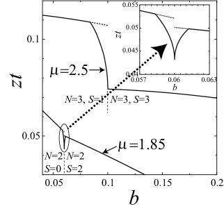
Figure 2: Phase boundary curves on a $b$-$zt$ plane for $\mu=2.5$ and for $\mu=1.85$. The dashed (solid) curves are obtained by the PMFA (GA). The inset is an enlargement around $b=0.06$ for $\mu=1.85$.

On the other hand, for $\mu=1.85$, the solid curve obtained by the GA has a sharp cusp structure around $b=0.06$ where the MI states with $S=0$ and $S=2$ are degenerated. The critical value of $zt$ just for $b=0.06$ is different from both of the two limiting values from the weak or strong magnetic field region obtained by the PMFA. The transition is a FOT near (but not just for) $b=0.06$. However, the SF order parameters become smaller when $b$ becomes closer to $0.06$, and finally the transition becomes a SOT just for $b=0.06$. In fact, by using a degenerate PMFA that assumes two MI states such that $|N,S-2\rangle$ and $|N,S\rangle$ as zeroth-order states, we obtain the critical value of $zt$ as $(zt_{\mathrm{d}eg})^{-1}=\frac{1}{2}\Big{[}a_{+}-\frac{a_{-}c}{2b_{-}}+\frac{1}{2}(1+\frac{a_{-}^{2}}{|b_{-}|})\sqrt{\frac{c^{2}-4b_{-}b_{+}}{a_{-}^{2}-b_{-}}}\Big{]}$, where $a_{\pm}\equiv(\alpha_{S,+}\pm\alpha_{S,-}+\alpha_{S-2,+}\pm\alpha_{S-2,-})/2$, $b_{\pm}\equiv[\alpha_{S,+}\pm\alpha_{S,-}-(\alpha_{S-2,+}\pm\alpha_{S-2,-})]^{2}/4\pm\beta^{2}$, and $c\equiv[(\alpha_{S,+}-\alpha_{S-2,+})^{2}-(\alpha_{S,-}-\alpha_{S-2,-})^{2}]/2$. Here, $\alpha_{S,\pm}\equiv f_{N,S,S}^{N+1,S+1,S\pm 1}+f_{N,S,S}^{N\mp 1,S\pm 1,S-1}+f_{N,S,S}^{N-1,S\mp 1,S\mp 1}$ and $\beta=\frac{{\langle N+1,S-1,S-1|{\hat{a}}_{-1}^{\dagger}|N,S,S\rangle}\langle N,S-2,S-2|{\hat{a}}_{1}|N+1,S-1,S-1\rangle}{E(N+1,S-1,S-1)-E(N,S,S)}+\frac{{\langle N-1,S-1,S-1|{\hat{a}}_{1}|N,S,S\rangle}\langle N,S-2,S-2|{\hat{a}}_{-1}^{\dagger}|N-1,S-1,S-1\rangle}{E(N+1,S-1,S-1)-E(N,S,S)}$. Here, $E(i,j,k)$ is the energy per site of an MI state $\Phi=|i,j,k\rangle$ and $f_{l,m,n}^{i,j,k}\equiv\frac{|\langle l,m,n|{\tilde{a}}|i,j,k\rangle|^{2}}{E(i,j,k)-E(l,m,n)}$, where ${\tilde{a}}$ is a creation or an annihilation operator which joins $|l,m,n\rangle$ and $|i,j,k\rangle$ matrix . The PMFA chooses $zt_{\mathrm{d}eg}$ as the critical value only when $zt_{\mathrm{d}eg}$ is smaller than the two limiting values from the weak or strong magnetic field. Furthermore, another condition $\Big{|}\big{[}c-a_{-}{\rm sgn}(b_{-})\sqrt{(c^{2}-4b_{-}b_{+})/(a_{-}^{2}-b_{-})}\big{]}/(2b_{-})\Big{|}<1$ must also be satisfied because the absolute values of the SF-order parameters must be non-negative. The latter condition is not satisfied in the case of $\mu=2.5$ in Fig. 2. It should also be noted that the same critical value as $zt_{\mathrm{d}eg}$ can be not only numerically but also analytically obtained by the GA including the states that emerge as zeroth-order or intermediate states in the degenerate PMFA calculation.

Superfluid properties— Figure 3 shows magnetization per site and FTNB as a function of magnetic field for $\mu=1.92$ and for a constant $zt=0.02$ parametersets . The FTNB is proportional to the experimental observables, such as the compressibility and the inverse square of the sound velocity Fisher . Both the magnetization and the FTNB curves can be clearly divided into four parts depending on the magnetic field. There are always discontinuous jumps of the differential magnetic susceptibility and the derivative of the FTNB on the boundaries between the four parts.

To clearly understand the magnetization and the FTNB curves, we also show phase boundary curves in Fig. 4, where the SF-MI transition is a SOT (FOT) under a magnetic field $b\leq 0.06$ or $0.0670<b$ ($0.06<b<0.0670$). The MI states $|N=2,S=0\rangle$ and $|N=2,S=2\rangle$ are degenerated at $b=0.06$ and the former (latter) is more favored under a weaker (stronger) magnetic field. For $zt=0.02$ in Fig. 4, the first region ($b<0.0462$) and the fourth region ($0.0612<b$) correspond to the MI phases $|N=2,S=0\rangle$ and $|N=2,S=2\rangle$, respectively, where the magnetization is constant and the FTNB is zero as shown in Fig. 3.

The SF phase in the second region $0.0462<b<0.0596$ has a perturbative character: The SF state is continuously connected to the nearest MI state, and the spin property of the system is close to that of the MI state. The inset of Fig. 4 indeed shows that $|f(2,2)|^{2}$, which is the amplitude of a high spin state $|N=2,S=2\rangle$ normalized as $|f(2,0)|^{2}+|f(2,2)|^{2}=1$, is almost negligible and that the lowest spin state $|N=2,S=0\rangle$ is dominant in the second region. This perturbative character originates from a SOT between the SF phase in the second region and the MI phase in the first region.

On the other hand, the SF in the third region has a non-perturbative character such that states with high spins are largely included, resulting in the large $\langle S_{z}\rangle$ as shown in Fig. 3. The inset of Fig. 4 shows that $|f(2,2)|^{2}$ is indeed large in the third region. This change of the SF character also affects the FTNB as shown in Fig. 3. It should also be noted the non-perturbative SF phase can also be characterized as a coherent-state-like character with a large kinetic energy as in the case of a zero magnetic field Kimura . This non-perturbative character is related to a FOT between the SF phase in the third region and the MI phase in the fourth region.

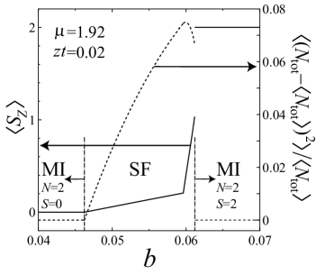
Figure 3: Magnetization per site $\langle S_{z}\rangle$ (solid curves) and fluctuation in the total number of bosons $\langle(N_{\mathrm{t}ot}-\langle N_{\mathrm{t}ot}\rangle)^{2}\rangle/\langle N_{\mathrm{t}ot}\rangle$ (dashed curves) as a function of magnetic field for $\mu=1.92$.

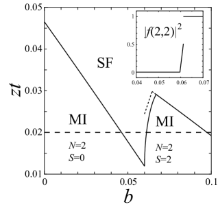
Figure 4: Phase boundary curves for $\mu=1.92$. The solid (short dashed) curve is obtained by the GA (PMFA). The long dashed line, which shows the $zt=0.02$ assumed in Fig. 3, intersects with the solid curve at $b=0.0462$ and $b=0.0612$. The inset shows $|f(2,2)|^{2}$ as a function of magnetic field (See text for the definition).

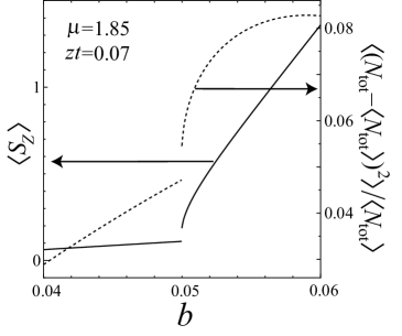
Figure 5: The same plot as in Fig. 3 for $\mu=1.85$ and $zt=0.07$.

We can see the crossover between the two SF phases in a wide parameter region when the SOT and FOT phase boundary curves coexist. For instance, the critical value of $zt$ for the SF-MI transition just at the boundary between MI phases with different spins has not to be necessary a local minimum as a function of magnetic field. Although not shown here, we indeed found a clear crossover between the non-perturbative and perturbative SF phases for $zt>0.075$ and $\mu=2.5$ around $b=0.1$ (See Fig. 2 for the phase boundary curve). Here, the critical value of $zt=0.075$ for $b=0.1$ is not a local minimum as a function of magnetic field.

Let us explain some details. There are no gaps on the curves of the magnetization and the FTNB at the boundary between the perturbative and non-perturbative SF phases in Fig. 3. On the other hand, there are gaps in the parameter region as shown in Fig. 5 for $\mu=1.85$ and $zt=0.07$, for which the phase boundary curves are shown in Fig 2. For $\mu=1.85$ and $zt=0.07$, the SF-MI transition occurs only once for $b\simeq 0.0274$ through a SOT. However, a FOT also occurs for a slightly larger $b$ and a slightly smaller $zt$, resulting in a crossover between the two kinds of SF phases for $zt=0.07$ gap .

We finally note that the GA neglects inter-site correlation effects, which could be important when $U_{2}$ is smaller than or comparable with $zt^{2}/U_{0}$ and/or when the dimension of the lattice is low. Although $zt^{2}/U_{0}$ is somewhat smaller or much smaller than $U_{2}$ in the typical parameter sets we have assumed in this paper parameter , a somewhat larger $U_{2}$ would more clearly justify the GA. A larger $U_{2}$ is also favorable from the experimental point of view. This is because both Zeeman energy and antiferromagnetic interaction energy become comparable under a stronger magnetic field and the interesting features clarified in this paper can be easily observed.

This work was supported by a Grant-in-Aid for the 21st Century COE Program of Waseda University (Physics of Systems with Self-Organization Composed of Multi-Elements).

References

- (1) M. Greiner et al., Nature 415, 918 (2002).
- (2) M.P.A. Fisher et al., Phys. Rev. B 40, 546 (1989).
- (3) K. Sheshadri et al. Europhys. Lett. 22, 257 (1993); J.K. Freericks and H. Monien, Phys. Rev. B 53, 2691 (1996).
- (4) D. Jaksch et al., Phys. Rev. Lett. 81, 3108 (1998).
- (5) For reviews, D. Vollhardt, Rev. Mod. Phys. 56, 99 (1984); A. Georges et al., ibid. 68, 13 (1996).
- (6) D.S. Rokhsar and B.G. Kotliar, Phys. Rev. B 44, 10328 (1991); W. Krauth, M. Caffarel and J.-P. Bouchaud, Phys. Rev. B 45, 3137 (1992); C. Schroll, F. Marquardt, and C. Bruder, Phys. Rev. A 70, 053609 (2004).
- (7) G.G. Batrouni, R.T. Scalettar and G.T Zimanyi, Phys. Rev. Lett. 65, 1765 (1990); W. Krauth and N. Trivedi, Europhys. Lett. 14, 627 (1991). See for bosons in harmonic traps, V.A. Kashurnikov, N.V. Prokof’ev, and B.V. Svistunov, Phys. Rev. A 66, 031601(R) (2002); G.G. Batrouni, et al., Phys. Rev. Lett. 89, 117203 (2002); S. Wessel et al, Phys. Rev. A 70, 053615 (2004).
- (8) T.-L. Ho, Phys. Rev. Lett. 81, 742 (1998); T. Ohmi and K. Machida, J. Phys. Soc. Jpn. 67, 1822 (1998); F. Zhou, Phys. Rev. Lett. 87, 080401 (2001); J.J. Garcia-Ripoll, M.A. Martin-Delgado, and J.I. Cirac Phys. Rev. Lett. 93, 250405 (2004); and references therein.
- (9) D.M. Stamper-Kurn et al., Phys. Rev. Lett. 80, 2027 (1998).
- (10) E. Demler and F. Zhou, Phys. Rev. Lett. 88, 163001 (2002).
- (11) A. Imambekov, M. Lukin, and E. Demler, Phys. Rev. A 68, 063602 (2003); M. Snoek and F. Zhou, Phys. Rev. B 69, 094410 (2004);
- (12) R. Cheng and J.-Q. Liang, unpublished (cond-mat/0506099).
- (13) A. Imambekov, M. Lukin, and E. Demler, Phys. Rev. Lett. 93, 120405 (2004); F. Zhou et al., Phys. Rev. B 70, 184434 (2004); H. Zhai and F. Zhou, unpublished (cond-mat/0501490).
- (14) D. van Oosten, P. van der Straten, and H.T.C. Stoof, Phys. Rev. A 63, 053601 (2001).
- (15) S. Tsuchiya, S. Kurihara, and T. Kimura, Phys. Rev. A 70, 043628 (2004).
- (16) T. Kimura, S. Tsuchiya, and S. Kurihara, Phys. Rev. Lett. 94, 110403 (2005).
- (17) K.V. Krutitsky and R. Graham, Phys. Rev. A 70, 063610 (2004); K.V. Krutitsky, M. Timmer, and R. Graham, Phys. Rev. A 71, 033623 (2005).
- (18) M. Rizzi et al., unpublished (cond-mat/0506098).
- (19) N. Uesugi and M. Wadati, J. Phys. Soc. Jpn. 72, 1041 (2003).
- (20) A.A. Svidzinsky and S.T. Chui, Phys. Rev. A 68, 043612 (2003).
- (21) The FTNB is equal to the fluctuation of number of bosons in a single site as within the GA.
- (22) The critical value of is generally finite at the phase boundary between MI states with the same and with different spins as shown in Fig. 2 because the FTNB is zero for sufficiently small .
- (23) For the matrix elements, see Refs. Uesugi ; Svidzinsky ; Tsuchiya .
- (24) The situation is simplified in this parameter set; there is no FOT under a weak magnetic field: the degenerate PMFA is not needed in order to determine the phase boundary.
- (25) As far as the authors know, the gaps can be finite only when the SOT and FOT coexist on the phase boundary around the same MI state as in the case for and .
- (26) We have typically assumed in this paper. This leads to for a three-dimensional cubic lattice ().