Simulations of Dense Atomic Hydrogen in the Wigner Crystal Phase

Abstract

Path integral Monte Carlo simulations are applied to study dense atomic hydrogen in the regime where the protons form a Wigner crystal. The interaction of the protons with the degenerate electron gas is modeled by Thomas-Fermi screening, which leads to a Yukawa potential for the proton-proton interaction. A numerical technique for the derivation of the corresponding action of the paths is described. For a fixed density of $r_{s}=200$, the melting is analyzed using the Lindemann ratio, the structure factor and free energy calculations. Anharmonic effects in the crystal vibrations are analyzed.

Proceedings article of the Study of Matter at Extreme Conditions (SMEC) conference in Miami, Florida
submitted to Journal of Physics and Chemistry of Solids (2005)

1 Introduction

Recent advances in high pressure experiments and computer simulations techniques have led to substantial progress in our understanding of the melting properties of solid hydrogen at high pressure. Using diamond anvil cell experiments, E. Gregoryanz et al. [1] extended the experimental determination of the melting line from 15 GPa [2] to 40 GPa. Bonev et al. combined the two-phase melting technique with ab initio simulations [3] and predicted that there is a maximum in the melting temperature around 80 GPa [4]. At these pressures, hydrogen is still in molecular form. The question of interest is whether the melting temperature keeps decreasing as the pressure is increased further, or if another phase appears and the melting temperature again increases.

From theoretical arguments, we know that atomic hydrogen eventually transforms into a Wigner crystal where the protons form a body centered cubic (b.c.c.) lattice. The focus of this work is to characterize this regime more accurately, to determine its melting line and to analyze by how much the known molecular solids phase and the Wigner crystal phase are separated on the pressure or density scale.

In this article, we study the Wigner crystal of protons using path integral Monte Carlo (PIMC). This technique allows us to characterize the quantum effects of the protons. The anharmonic effects in the lattice vibrations are also included accurately. While at much higher temperature and lower density, one can describe the electrons from first principles [5]. For this work, we instead approximate the electron-proton interaction using Thomas-Fermi theory. This leads to an effective Yukawa potential for the proton-proton interaction,

$$V_{Y}(r)=\frac{\mathbf{e}^{2}}{r}e^{-r/D_{s}}\;,$$ (1)

where the screening length $D_{s}$ is given by [6],

$$D_{s}=\left(\frac{\pi}{12}\right)^{1/3}\left(\frac{r_{s}}{a_{0}}\right)^{1/2}\,a_{0}\;,$$ (2)

and $r_{s}$ is the Wigner-Seitz radius, $\frac{4}{3}\pi r_{s}^{3}=V/N$. Throughout this work, we will use units of nuclear Bohr radii, $a_{0}=4\pi\epsilon_{0}\hbar^{2}/m_{p}\mathbf{e}^{2}$ = 2.9$\times$$10^{-14}$ m and nuclear Hartrees, Ha = $\mathbf{e}^{2}/(4\pi\epsilon_{0}a_{0})$ = 8.0$\times$$10^{-15}$ J = $5.8\times 10^{8}$ K $k_{b}$, which are by a factor by $m_{p}/m_{e}=1836$ shorter, or larger respectively, than the usual atomic units.

Jones and Ceperley [7] used PIMC to study quantum melting in Coulomb systems where the electrons were assumed to form a rigid background. We extend their work by introducing the Yukawa potential in order to understand how the electronic screening affects the stability of the Wigner crystal.

2 Path integral Monte Carlo

The thermodynamic properties of a many-body quantum system at finite temperature can be computed by averaging over the density matrix, $\hat{\rho}=e^{-\beta\hat{H}},\beta=1/k_{\rm b}T$. Path integral formalism [8] is based on the identity,

$$\hat{\rho}\equiv e^{-\beta\hat{H}}=\left[e^{-\frac{\beta}{M}\hat{H}}\right]^{M}\;,$$ (3)

where $M$ is a positive integer. Insertion of complete sets of states between the $M$ factors leads to the usual imaginary time path integral formulation, written here in real space,

$$\rho({\bf R},{\bf R}^{\prime};\beta)=\int\ldots\int d{\bf R}_{1}\ldots d{\bf R}_{M-1}\;\rho({\bf R},{\bf R}_{1};\tau)\ldots\rho({\bf R}_{M-1},{\bf R}^{\prime};\tau)\;,$$ (4)

where $\tau=\beta/M$ is the time step, and ${\bf R}$ is a collective coordinate including all particles, ${\bf R}=\{{\bf r}_{1},\ldots,{\bf r}_{N}\}$. Each of the $M$ steps in the path now has a high temperature density matrix $\rho({\bf R}_{k},{\bf R}_{k+1};\tau)$ associated with it. The integrals are evaluated by Monte Carlo methods. For the densities under consideration, we can neglect exchange effects of the protons and represent them by distinguishable particles. Given these constraints, PIMC is an exact technique and free of uncontrolled approximations (assuming the Yukawa potential is valid). This technique includes the correct phonon excitations in the presence of anharmonic effects, which we will discuss later.

2.1 Action for an Isolated Pair of Particles

The action plays a central role in PIMC since it determines the weights of paths. We will describe a novel approach for its derivation, which we found to be more accurate for Yukawa systems than previous techniques. First we discuss the action for an isolated pair of particles, and then we introduce periodic boundary conditions commonly used in many-body simulations.

Typically, one approximates the high-temperature many-body density matrix,
$\rho({\bf R},{\bf R}^{\prime};\tau)$, as a product of exact pair density matrices which can be motivated using the Feynman-Kac (FK) formula,

$$\frac{\rho({\bf R},{\bf R}^{\prime};\tau)}{\rho_{0}({\bf R},{\bf R}^{\prime};\tau)} = \left<e^{-\int_{0}^{\tau}dt\sum_{i<j}V_{Y}({\bf r}_{ij})}\right>_{\rm{\bf R}\to{\bf R}^{\prime}}=\left<\prod_{i<j}e^{-\int_{0}^{\tau}dtV_{Y}({\bf r}_{ij})}\right>_{\rm{\bf R}\to{\bf R}^{\prime}}$$ (5)

$$\approx \prod_{i<j}\left<e^{-\int_{0}^{\tau}dtV_{Y}({\bf r}_{ij})}\right>_{\rm{\bf r}_{ij}\to{\bf r}_{ij}^{\prime}}\equiv e^{-\sum_{i<j}U_{Y}({\bf r}_{ij},{\bf r}_{ij}^{\prime};\tau)},$$ (6)

where $\rho_{0}({\bf R},{\bf R}^{\prime};\tau)$ is the free particle density matrix. $U_{Y}({\bf r}_{ij},{\bf r}_{ij}^{\prime};\tau)$ is the pair action corresponding to all paths separated by ${\bf r}_{ij}$ at imaginary time $t=0$ and by ${\bf r}^{\prime}_{ij}$ at $t=\tau$. An approximation is introduced when one makes the assumption that the different pair interactions can be averaged by independent Brownian random walks, denoted by brackets $\left<\ldots\right>$. The pair action approximation is exact for two particle problem. However, higher-order correlations are left out, which must be recovered in the many-body PIMC simulations using a sufficiently small time step $\tau$.

The pair action, $U_{Y}$, can be computed by three different methods. 1) For certain potentials where the eigenstates are known in analytical form, e.g. for the Coulomb potential, the action can be derived from the sum of state [9]. However to our knowledge, for the Yukawa potential they are not known analytically. 2) In the matrix squaring technique [10], one represents the density matrix on a grid and successively lowers the temperature by performing a one-step path integration. This method can be applied to arbitrary potentials. 3) For the Yukawa potential, we found it advantageous to use the FK formula to derive the pair action. Computationally, it is a bit more expansive than matrix squaring but it does not introduce grid errors that we found difficult to control in case of the Yukawa potential. The FK approach is also applicable to arbitrary potentials unless they exhibit an attractive singularity, which is discussed further in [11].

In FK approach one derives the action $U_{Y}({\bf r},{\bf r}^{\prime};\beta)$ stochastically by generating an ensemble of random paths according to the free particle action $U_{0}({\bf r},{\bf r}^{\prime};\beta)$ that begin at ${\bf r}$ and terminate at ${\bf r}^{\prime}$,

$$e^{-(U_{Y}-U_{0})}=\left<e^{-\tau/2\sum_{i=1}^{M}[V_{Y}({\bf r}_{i-1})+V_{Y}({\bf r}_{i})]}\right>_{U_{0}({\bf r},{\bf r}^{\prime};\beta)}\;.$$ (7)

The free-particle paths can be generated by a bisection algorithm [12]. We found that $M=\beta/\tau=32$ time steps was sufficient for the Yukawa potential.

To determine the kinetic energy in simulations, one also needs the derivative of the action with respect to $\beta$, which can be evaluated from the same set of paths,

$$\frac{\partial}{\partial\beta}(U_{Y}-U_{0})=\left<e^{-\sum_{i}\tau V_{Y}({\bf r}_{i})}\frac{1}{M}\sum_{i=1}^{M}\left[V_{Y}({\bf r}_{i})+\frac{1}{2}({\bf r}_{i}-{\bf r}_{i}^{\rm Cl})\cdot\nabla V_{Y}({\bf r}_{i})\right]\right>_{U_{0}({\bf r},{\bf r}^{\prime};\beta)}.$$ (8)

where ${\bf r}_{i}^{\rm Cl}$ represents the classical path between the two end points.

The FK formula yields the action for only one specific pair of ${\bf r}$ to ${\bf r}^{\prime}$. For the diagonal action, ${\bf r}={\bf r}^{\prime}$, we map out a whole grid of points beginning from a small value near the origin to large values (several times the thermal de Broglie wavelength given by $\sqrt{2\pi\hbar^{2}\beta/m}$). Typically, we use a logarithmic grid with about 500 points. For large $r$, the action approaches the classical limit given by the primitive approximation,

$$U_{Y}({\bf r},{\bf r}^{\prime};\beta)\approx\frac{\beta}{2}\left[V_{Y}({\bf r})+V_{Y}({\bf r}^{\prime})\right]\;,$$ (9)

which is shown in Fig. 1.

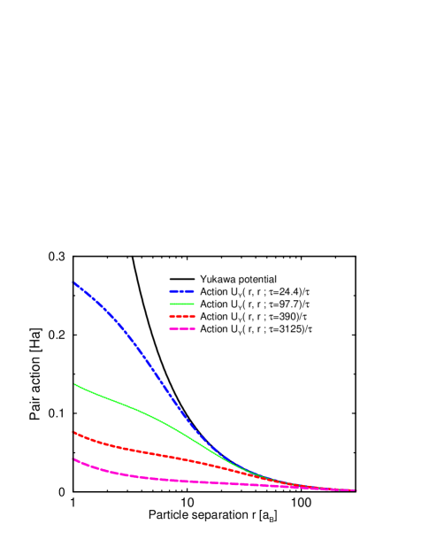
Figure 1: The pair action $U_{Y}(r,r^{\prime}=r;\tau)$ scaled by by $1/\tau$ is compared with the corresponding Yukawa potential as a function path separation, $r$. The Yukawa screening length of $D_{s}=387$ represents the electronic screening of the proton interaction in hydrogen at a density of $r_{s}=200$. The action converges to the primitive approximation, Eq. 9, for large $r$ and small $\tau$. At small $r$, quantum fluctuations remove the singularity present in the Yukawa potential and lead to a linear dependence on $r$, which is known as the cusp condition.

Statistical uncertainties in the resulting action are intrinsic to the FK approach. We found that $10^{6}$ paths yield sufficiently small error bars. However, any noise in tabulated action values is impractical for the subsequent interpolation in PIMC simulations. To eliminate this problem, we use the same random paths for all grid points in the table. This does not remove the uncertainty but prevents noise in the tables.

Including off-diagonal density matrix elements in PIMC simulations allows one to use larger time steps, which makes the simulation more efficient. However, the off-diagonal terms are more difficult to obtain with the FK approach, which is one of the limitations of the approach. Here, we only consider the leading term in an expansion of the action [12],

$$U_{Y}({\bf r},{\bf r}^{\prime};\beta)\approx U_{Y}(q,q;\beta)+s^{2}\>\xi(q;\beta)\;+\;\ldots$$ (10)

where $q=\frac{1}{2}(|{\bf r}|+|{\bf r}^{\prime}|)$ and $s=|{\bf r}-{\bf r}^{\prime}|$. It turns out that it is more efficient to derive $\xi$ from finite differences in $s$ rather than evaluating an analytical expression. Having completed our derivation for the action of an isolated pair of particles, we now consider a system with periodic boundary conditions.

2.2 Pair Action in Periodic Boundary Conditions

In our PIMC simulations, we use $N=250$ particles, which are initially placed on the sites of a b.c.c. lattice. For the density under consideration ($r_{s}=200$), the corresponding screening length for hydrogen ($D_{s}=387.667$) is comparable in magnitude to the length of the simulation cell $L=1218.59$. Consequently, long-range effects from periodic image particles are far from negligible, and significant care must be taken to derive results in the thermodynamic limit.

The total potential energy for a system of $N$ particles interacting via the Yukawa potential $V_{Y}(r)$ is given by [13],

$$V=\sum_{i>j}\sum_{\mathbf{L}}V_{Y}({\bf r}_{ij}+{\mathbf{L}})\;+\;\frac{1}{2}\sum_{i}\sum_{{\mathbf{L}}\neq 0}V_{Y}({\mathbf{L}})\;,$$ (11)

where ${\bf r}_{ij}={\bf r}_{i}-{\bf r}_{j}$ and ${\mathbf{L}}$ is a lattice vector. Instead of representing long-range terms, $V_{P}({\bf r})=\sum_{\mathbf{L}}V_{Y}({\bf r}+{\mathbf{L}})$, on a 3D table [14], we adopt the optimized Ewald [15], technique by Natoli and Ceperley [16] and express the potential as a sum of one real-space image, $W(|{\bf r}|)$, and a number of Fourier components,

$$V_{P}({\bf r})\equiv\sum_{\mathbf{L}}V_{Y}({\bf r}+{\mathbf{L}})\approx W(|{\bf r}|)+\sum_{|\mathbf{k}|\leq k_{c}}y_{\mathbf{k}}e^{+i\mathbf{k}{\bf r}}.$$ (12)

Following Natoli and Ceperley [16], we express $W$ as a linear combination of fifth-order polynomials, $W(|{\bf r}|)=\sum_{n}a_{n}f_{n}(|{\bf r}|)$, which is known as a locally piecewise-quintic Hermite interpolant. The fit coefficients $a_{n}$ and $y_{\mathbf{k}}$ can be derived by minimizing the $\chi^{2}$ deviation,

$$\chi^{2}=\frac{1}{\Omega}\int_{\Omega}d^{3}{\bf r}\left[V_{P}({\bf r})-\sum_{n}a_{n}f_{n}(|{\bf r}|)-\sum_{|\mathbf{k}|\leq k_{c}}y_{\mathbf{k}}e^{+i\mathbf{k}{\bf r}}\right]^{2}\;,$$ (13)

where $\Omega=L^{3}$ is the volume of the unit cell. For the Fourier coefficients this directly yields,

$$y_{\mathbf{k}}=v_{\mathbf{k}}-\sum_{n}a_{n}f_{n\mathbf{k}}\;,~{}~{}~{}~{}~{}~{}\mbox{with}~{}~{}~{}~{}~{}~{}v_{\mathbf{k}}=\frac{1}{\Omega}\int_{\Omega}d^{3}{\bf r}V_{P}({\bf r})e^{-i\mathbf{k}{\bf r}}\;,$$ (14)

where $v_{\mathbf{k}}$ and $f_{n\mathbf{k}}$ are the corresponding Fourier transforms. Deviating from [16], we derive the coefficients $a_{n}$ from the following set of linear equations, $m=\{1,\ldots,n\}$,

$$\left[v_{m}-\sum_{|\mathbf{k}|\leq k_{c}}v_{\mathbf{k}}f_{m\mathbf{k}}\right]=\sum_{n}a_{n}\left[f_{nm}-\sum_{|\mathbf{k}|\leq k_{c}}f_{n\mathbf{k}}f_{m\mathbf{k}}\right].$$ (15)

$v_{m}$ and $f_{nm}$ are overlap integrals, $f_{nm}=\frac{1}{\Omega}\int_{\Omega}d^{3}{\bf r}f_{n}({\bf r})f_{m}({\bf r})$, and

$$v_{m} = \frac{1}{\Omega}\int_{\Omega}d^{3}{\bf r}\;V_{P}({\bf r})\,f_{m}(|{\bf r}|)=\frac{1}{\Omega}\sum_{\mathbf{L}}\int_{\Omega}d^{3}{\bf r}\;V_{Y}({\bf r})\,f_{m}(|{\bf r}|)$$ (16)

$$= \frac{4\pi}{\Omega}\int dr\,r^{2}\,V_{Y}(r)f_{m}(r)\;+\;\sum_{{\mathbf{L}}\neq 0}\frac{2\pi}{\Omega L}\int dr\,r\,f_{m}(r)\int_{L-r}^{L+r}dq\,q\,V_{Y}(q)\;.$$ (17)

In the last expression, one must sum over a sufficiently large number of images until the interaction is completely screened, $|{\mathbf{L}}|\gg D_{s}$. Computing the coefficients $a_{n}$ using the real-space integration in Eq. 17 is more efficient and accurate than the Fourier integration employed in [16]. Our approach also works well for the Coulomb problem, which was the motivation for the [16] work. In this case, the Ewald potential replaces $V_{P}$ in Eq. 13.

This optimized Ewald approach provides us with an accurate representation of the periodic functions leading to efficient many-body simulations. We apply it to the Yukawa potential, $V_{Y}$, to the corresponding pair action, $U_{Y}$, and also to the kinetic energy term, $\left(\frac{dU_{Y}}{d\beta}-V_{Y}\right)$, unless it is very small for $r=L/2$. Typically, we use between 10 and 20 shells of $k$ vectors.

3 Results

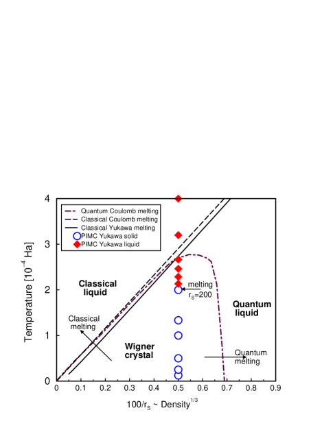
Figure 2: Phase diagram for Wigner crystal. The dashed lines show the classical melting line, $\Gamma=172$, and quantum melting line for Coulomb systems computed by Jones and Ceperley [7] with PIMC. The solid lines show the classical melting line for the Yukawa system with the screening length chosen for hydrogen. Our PIMC simulations at $r_{s}=200$ ($\circ$ and $\diamond$) show a significant reduction in the melting temperature below the classical value due to the quantum effects of the protons.

The phase diagram in Fig. 2 relates our simulations at a fixed density of $r_{s}=200$ to the classical Yukawa melting computed by Hamaguchi, the classical Coulomb melting line given by $\Gamma=\frac{\mathbf{e^{2}}}{r_{s}k_{b}T}=172$, and the quantum melting for Coulomb systems [7].

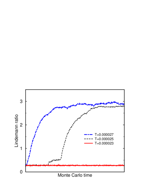
Figure 3: The evolution of the Lindemann ratio is shown for the three Monte Carlo simulations in the vicinity of the melting temperature.

The most straightforward way to detect melting in the simulation is to monitor the instantaneous value of the Lindemann ratio, $\gamma=\sqrt{\left<u^{2}\right>}/r_{NN}$, which relates the average displacement of a particle from its original lattice site to the nearest neighbor distance. Fig. 3 shows the Lindemann ratio for three Monte Carlo simulations. At the beginning of each simulation, the particles are in the classical b.c.c. ground state. For temperatures sufficiently above the melting line, the system melts instantly. For temperatures only slightly above the melting line, the simulation shows a meta-stable superheated solid, which might melt at some point during the MC simulation, as the black dashed line indicates. The time it takes to melt depends not only on temperature, but also on system size, the type of MC moves, and the MC random numbers, thereby making this criterion impractical for determining the melting temperature.

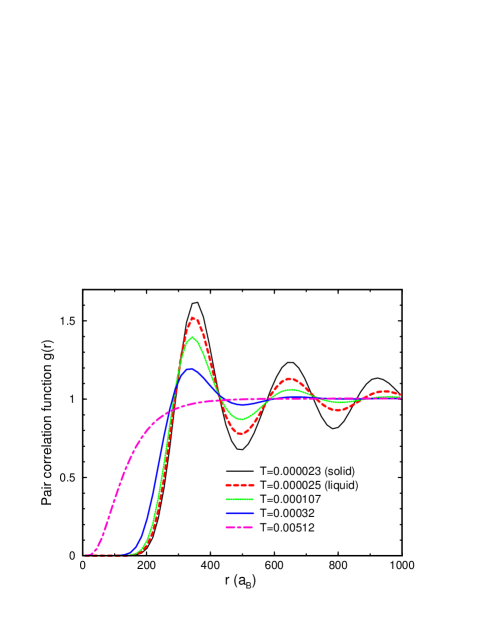
Figure 4: Pair correlation functions, $g(r)$, for different temperatures.

Fig. 4 shows a series of pair correlation functions, $g(r)$, for simulations at different temperatures. The magnitude of the oscillations in the $g(r)$ show a significant temperature dependence in the liquid phase. However, there is only a small change upon melting and all $g(r)$ functions in the solid phase are practically identical to the example shown for T=2.3$\times$10^-5.

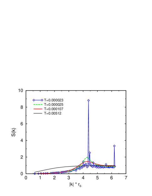
Figure 5: The sharp peaks in the structure factor, $S(k)$, disappear when the system melts and a pattern typical for a liquid appears. This transition coincides with the increase in the Lindemann ratio.

Compared to the pair correlation function, the structure factor, $S(k)$, shows significant changes upon melting (Fig. 5). The disappearance of the peaks coincides with the increase in the Lindemann ratio beyond stable value of approximately 0.28. However, neither method can determine whether a simulation is in the meta-stable state. They only lead to an upper bound of the melting temperature. To determine the thermodynamic phase boundary, one needs the free energy in both phases, which can be obtained through thermodynamic integration of the internal energies.

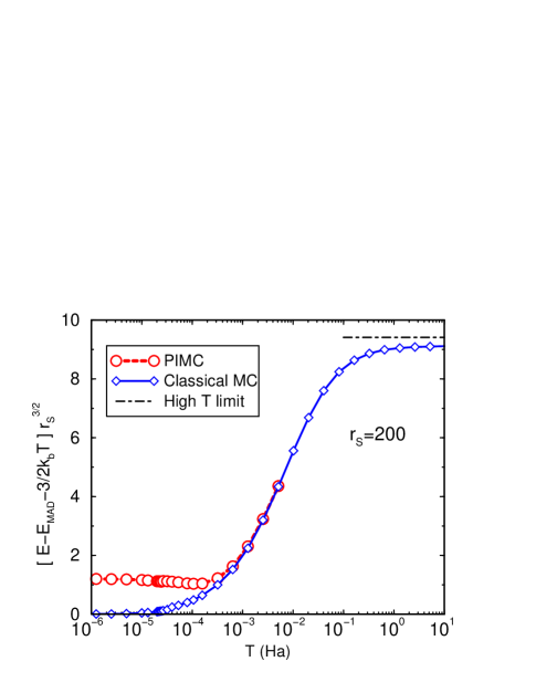
Figure 6: The internal energy per particle is shown as a function of temperature. The classical kinetic energy and the Madelung term have been removed.

Fig. 6 compares PIMC internal energies with results from corresponding classical MC that we have performed. At high temperature when the thermal de Broglie wavelength is short compared to the inter-particle spacing, the protons behave classically and the PIMC energies approach results from classical MC simulations. At low T, both result differ substantially due to the zero point motion. The analytical high T limit [14] is not reached exactly, due to finite size effects.

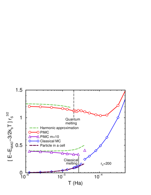
Figure 7: Low temperature region of Fig. 6. Results from the harmonic lattice approximation and from a classical particle-in-a-cell model have been added. Furthermore, PIMC and harmonic results for particles with mass=10 instead of 1 have been included to demonstrate that the harmonic approximation becomes more accurate as zero point fluctuations are reduced.

In Fig. 7, we compare MC results with our results derived from the harmonic lattice approximation and the particle-in-a-cell (PIC) model. In the PIC approximation, one assumes that the thermal motion of the particles are uncorrelated. One freezes all particles in the supercell except one and derives all thermodynamic variables from the motion of this single classical particle. The PIC internal energies agree remarkably well with the corresponding classical MC results. A generalization to the quantum case is not straightforward. If one simply considers a quantum particle, represented by a path in a lattice of frozen particles then the resulting kinetic energies are far too high (worse than the harmonic approximation) because the remaining classical particles provide too high of a confining force due to the missing quantum fluctuations.

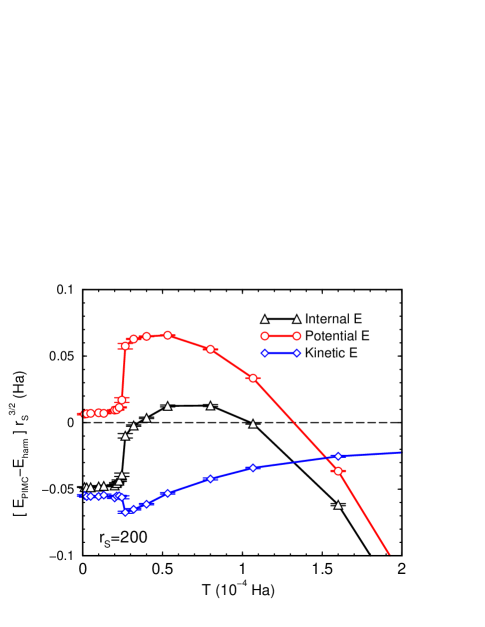
Figure 8: Difference in internal, kinetic, and potential energy between PIMC and the harmonic lattice approximation. The sharp kinks near T=2.5$\times$10^-5 indicate the melting transition.

Fig. 7 also shows results from the harmonic lattice approximation for a unit cell of corresponding size. Harmonic internal energies are significantly overestimated, primarily due to errors in the kinetic energy as demonstrated in Fig. 8. The zero point motion of the protons is large enough so that paths travel into regions of the potential where the harmonic approximation is not longer valid. A comparison of the PIMC Lindemann ratios and the harmonic values shows that the harmonic approximation localizes the particles too much, thereby increasing the kinetic energy.

To further support this conclusion, we perform PIMC and harmonic calculation with particles 10 times as heavy. Fig. 7 shows that the agreement improves substantially.

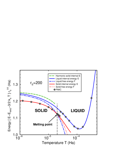
Figure 9: Internal and free energies, $E$ and $F$, are shown for the solid and liquid phase.

Fig. 9 shows the internal PIMC energies along with the free energies obtained from thermodynamic integration. The solid free energies agree very well with solid internal energies until melting, which suggest that each phonon mode is in its ground state, and excitation in the phonon spectra leads directly to melting. At low T, the free energies of the crystalline state are lower than the extrapolated values for the liquid, which means the solid phase is stable and the density of $r_{s}=200$ is not yet high enough to reach the quantum melting transition (see Fig. 2).

At T=2.0$\times$10^-5 the free energies of both phases match, which determines the thermodynamic melting point. This corresponds to a temperature of 11,700 K and a hydrogen mass density of 2,100 g cm^-3.

Fig. 9 also shows that a number of simulations that appeared to be stable were actually meta-stable, which can also occur in classical simulations (Fig. 7). The melting temperature of 2.0$\times$10^-5 is significantly below the corresponding classical value of 2.7$\times$10^-5, which suggests that quantum effects are important. However, a finite size extrapolation remains to be done.

4 Conclusions

In this article, we used many-body computer simulations of protons interacting via a Yukawa potential to model dense atomic hydrogen in the regime of the Wigner crystal. Path integral Monte Carlo simulations were employed to capture the quantum effects of the protons. Electronic screening effects were treated in the Thomas-Fermi approximation, which distinguishes our results from the earlier work by Jones and Ceperley [7].

We use the Lindemann ratio, pair correlation functions, and the structure factor to study the stability of the Wigner crystal and to detect melting. We observed that the system can remain in a meta-stable state of a super-heated crystal during the entire course of a PIMC simulation, which makes a direct determination of the melting temperature very difficult.

Instead, a reliable melting temperature can be obtained by matching of the free energies of both phases, which were derived by thermodynamic integration of the PIMC internal energies. For the density under consideration, $r_{s}=200$, we found that the quantum Yukawa systems melts at significantly lower temperatures than the corresponding classical system.

Furthermore, we compared our PIMC results with other more approximate techniques. The harmonic lattice approximation overestimates the kinetic energies significantly because the zero point motion of the protons is strong enough so that anharmonic effects in the crystal field become relevant. We also compared with a classical particle-in-a-cell model and found good agreement with classical MC simulation. However this method cannot be generalized easily to the case of quantum protons.

We plan to extend our analysis to other densities and to derive a phase diagram that indicates the stability of the Wigner crystal of nuclei in the presence of electronic screening effects. A careful analysis of finite size effects also remains to be done. Future theoretical work on dense atomic hydrogen will need to describe the electronic properties on a more fundamental level. Coupled ion-electron Monte Carlo is one promising approach [17].

5 Acknowledgments

We would like to acknowledge stimulating discussions with J. Kohanoff and M. Magnitskaya. R.L.G. received support from the National Science Foundation’s Research Experiences for Undergraduates program at the Carnegie Institution of Washington.

References

- [1] E. Gregoryanz, A. F. Goncharov, K. Matsuishi, H. Mao, and R. J. Hemley. Phys. Rev. Lett., 90:175701, 2003.
- [2] F. Datchi, P. Loubeyre, and R. LeToullec. Phys. Rev. B, 61:6535, 2000.
- [3] Tadashi Ogitsu, Eric Schwegler, Francois Gygi, and Giulia Galli. Nature, 91:175502, 2003.
- [4] S.A. Bonev, E. Schwegler, T. Ogitsu, and G. Galli. Nature, 431:669, 2004.
- [5] B. Militzer and D. M. Ceperley. Phys. Rev. Lett., 85:1890, 2000.
- [6] N. W. Ashcroft and N. D. Mermin. Solid State Physics. Harcourt, Inc., Orlando, FL, 1976.
- [7] M. D. Jones and D. M. Ceperley. Phys. Rev. Lett., 76:4572, 1996.
- [8] R. P. Feynman. Phys. Rev., 90:1116, 1953.
- [9] E. L. Pollock. Comp. Phys. Comm., 52 :49, 1988.
- [10] R. G. Storer. J. Math. Phys., 9:964, 1968.
- [11] B. Militzer and E. L. Pollock. Phys. Rev. B, 71:134303, 2005.
- [12] D. M. Ceperley. Rev. Mod. Phys., 67:279, 1995.
- [13] M.P. Allen and D.J. Tildesley. Computer Simulation of Liquids. Oxford University Press, New York, 1987.
- [14] S. Hamaguchi, R. T. Farouki, and D. H. E. Dubin. Phys. Rev. E, 56:4671, 1997.
- [15] P.P. Ewald. Ann. Phys., 54:557, 1917.
- [16] V. Natoli and D. M. Ceperley. J. Comp. Phys., 117:171–178, 1995.
- [17] C. Pierleoni, D. M. Ceperley, and M. Holzmann. Phys. Rev. Lett., 93:146402, 2004.