Introduction to the Keldysh Formalism and Applications to Time-Dependent Density-Functional theory

Abstract

This paper gives an introduction to the Keldysh formalism, with emphasis on its usefulness in time-dependent density functional theory. In the first part we introduce the Keldysh contour and the one-particle Green function defined on this contour. We then discuss how to combine and manipulate functions with time-arguments on the contour. The effects of electron-electron interaction can be taken systematically into account, as we illustrate by propagating the Kadanoff-Baym equations for the second-order self-energy approximation. It is important to use conserving approximations such that the evolution of the electron density, momentum, and total energy agrees with the macroscopic conservation laws. One of the main topics in this paper is the non-interacting Green function, which is the relevant quantity for time-dependent density functional theory. We discuss this Green function in detail, and show how the Keldysh contour in a simple way allows us to derive the time-dependent Kohn-Sham potential from an action functional. The formalism in a similar way leads to response functions that obey the causality principle. To illustrate these points, we discuss the time-dependent optimized effective potential equations.

I Introduction

We will in this paper give an introduction to the Keldysh formalism, which is an extremely useful tool for first-principles studies of nonequilibrium many-particle systems. Of particular interest for TDDFT is the relation to non-equilibrium Green functions (NEGF), which allows us to construct exchange-correlation potentials with memory by using diagrammatic techniques. For many problems, such as, e.g., quantum transport or atoms in intense laser pulses, one needs exchange-correlation functionals with memory, and Green function techniques offer a systematic method for developing these. The Keldysh formalism is also necessary for defining response functions in TDDFT and for defining an action functional needed for deriving TDDFT from a variational principle. We will in this section give an introduction to the nonequilibrium Green function formalism, intended to illustrate the usefulness of the theory. The formalism does not differ much from ordinary equilibrium theory, the main difference being that all time-dependent functions are definied for time-arguments on a contour, known as the Keldysh contour.

The Green function, $G(\vec{r},t;\vec{r}^{\prime},t^{\prime})$ is a function of two space- and time-coordinates, and is obviously more complicated than the one-particle density $n(\vec{r},t)$, which is the main ingredient in TDDFT. However, the advantage of the NEGF methods is that we can systematically improve the approximations by taking into account particular physical processes (represented in the form of Feynman diagrams) that we believe to be important. The Green function provides us directly with all expectation values of one-body operators (such as the density and the current), and also the total energy, ionization potentials, response functions, spectral functions, etc.. In relation to TDDFT, this is useful not only for developing orbital functionals and exchange-correlation functionals with memory, but also for providing insight in the exact properties of the non-interacting Kohn-Sham system.

In the following, we shall focus on systems that are initially in thermal equilibrium. We will start by introducing the Keldysh contour and the nonequilbrium Green functions, and then explain how to combine and manipulate functions with time variables on the contour. While we in TDDFT take exchange- and correlation-effects into account through $v_{\mathrm{xc}}[n]$, the corresponding quantity in Green function theory is the self-energy $\Sigma[G]$. Just like $v_{\mathrm{xc}}$, the self-energy functional must be approximated. For a given functional $\Sigma[G]$, it is important that the resulting observables obey the macroscopic conservation laws, such as, e.g., the continuity equation. These approximations are known as conserving, and will be discussed briefly. In the last part of this section we will discuss the applications of the Keldysh formalism in TDDFT, including the relation between $\Sigma$ and $v_{\mathrm{xc}}$, the derivation of the Kohn-Sham equations from an action functional, and the derivation of an $f_{\mathrm{xc}}$ functional. As an illustrative example, we will discuss the time-dependent exchange-only optimized effective potential approximation.

II The Keldysh Contour

In quantum mechanics we associate with any observable quantity $O$ a hermitean operator $\hat{O}$. The expectation value ${\rm Tr}\,\{\hat{\rho}_{0}\hat{O}\}$ gives the value of $O$ when the system is described by the density operator $\hat{\rho}_{0}$ and the trace denotes a sum over a complete set of states in Hilbert space. For an isolated system the Hamiltonian $\hat{H}_{0}$ does not depend on time, and the expectation value of any observable quantity is constant, provided $[\hat{\rho}_{0},\hat{H}_{0}]=0$. In these notes we want to discuss how to describe systems that are isolated for times $t<0$, such that $\hat{H}(t<0)=\hat{H}_{0}$, but disturbed by an external time-dependent field at $t>0$. The expectation value of $\hat{O}$ at $t>0$ is then given by the average on the initial density operator $\hat{\rho}_{0}$ of the operator $\hat{O}$ in the Heisenberg representation,

$$O(t)=\langle\hat{O}_{H}(t)\rangle\equiv{\rm Tr}\,\{\hat{\rho}_{0}\hat{O}_{H}(t)\}={\rm Tr}\,\{\hat{\rho}_{0}\hat{S}(0;t)\hat{O}\hat{S}(t;0)\},$$ (1)

where the operator in the Heisenberg picture has a time-dependence according to $\hat{O}_{H}(t)=\hat{S}(0;t)\hat{O}\hat{S}(t;0)$. The evolution operator $\hat{S}(t;t^{\prime})$ is the solution of the equations

$$i\frac{\mathrm{d}}{\mathrm{d}t}\hat{S}(t;t^{\prime})=\hat{H}(t)\hat{S}(t;t^{\prime})\qquad\mbox{and}\qquad i\frac{\mathrm{d}}{\mathrm{d}t^{\prime}}\hat{S}(t;t^{\prime})=-\hat{S}(t;t^{\prime})\hat{H}(t^{\prime}),$$ (2)

with the boundary condition $\hat{S}(t;t)=1$. It can be formally written as

$$\hat{S}(t;t^{\prime})=\left\{\begin{array}[]{ll}T\,e^{-i\int_{t^{\prime}}^{t}d\bar{t}\,\hat{H}(\bar{t})}&\quad t>t^{\prime}\\ \overline{T}\,e^{-i\int_{t^{\prime}}^{t}d\bar{t}\,\hat{H}(\bar{t})}&\quad t<t^{\prime}\end{array}\right..$$ (3)

In Eq. (3), $T$ is the time-ordering operator that rearranges the operators in chronological order with later times to the left; $\overline{T}$ is the anti-chronological time-ordering operator. The evolution operator satisfies the group property $\hat{S}(t;t_{1})\hat{S}(t_{1};t^{\prime})=\hat{S}(t;t^{\prime})$ for any $t_{1}$. Notice that if the Hamiltonian is time-independent in the interval between $t$ and $t^{\prime}$, then the evolution operator becomes $\hat{S}(t;t^{\prime})=e^{-i\hat{H}(t-t^{\prime})}$. If we now let the system be initially in thermal equilibrium, with an inverse temperature $\beta\equiv 1/k_{B}T$ and chemical potential $\mu$, the initial density matrix is $\hat{\rho}_{0}=e^{-\beta(\hat{H}_{0}-\mu\hat{N})}/{\rm Tr}\,\{e^{-\beta(\hat{H}_{0}-\mu\hat{N})}\}$. Assuming that $\hat{H}_{0}$ and $\hat{N}$ commute, $\hat{\rho}_{0}$ can be rewritten using the evolution operator $\hat{S}$ with a complex time-argument, $t=-i\beta$, according to $\hat{\rho}_{0}=e^{\beta\mu\hat{N}}\hat{S}(-i\beta;0)/{\rm Tr}\,\{e^{\beta\mu\hat{N}}\hat{S}(-i\beta;0)\}$. Inserting this expression in (1), we find

$$O(t)=\frac{{\rm Tr}\,\left[e^{\beta\mu\hat{N}}\hat{S}(-i\beta;0)\hat{S}(0;t)\hat{O}\hat{S}(t;0)\right]}{{\rm Tr}\,\left[e^{\beta\mu\hat{N}}\hat{S}(-i\beta;0)\right]}.$$ (4)

Reading the arguments in the numerator from the right to the left, we see that we can design a time-contour $\gamma$ with a forward branch going from $0$ to $t$, a backward branch coming back from $t$ and ending in $0$, and a branch along the imaginary time-axis from $0$ to $-i\beta$. This contour is illustrated in Fig. 1. Note that the group property of $\hat{S}$ means that we are free to extend this contour up to infinity. We can now generalize (4), and let $z$ be a time-contour variable on $\gamma$. Letting the variable $\bar{z}$ run along this same contour, (4) can be formally recast as

$$O(z)=\frac{{\rm Tr}\,\left[e^{\beta\mu\hat{N}}T_{\mathrm{c}}\left\{e^{-i\int_{\gamma}\mathrm{d}\bar{z}\,\hat{H}(\bar{z})}\;\hat{O}(z)\right\}\right]}{{\rm Tr}\,\left[e^{\beta\mu\hat{N}}T_{\mathrm{c}}\left\{e^{-i\int_{\gamma}\mathrm{d}\bar{z}\,\hat{H}(\bar{z})}\right\}\right]}.$$ (5)

The contour ordering operator $T_{\mathrm{c}}$ moves the operators with “later” contour variable to the left. In (5), $\hat{O}(z)$ is not the operator in the Heisenberg representation [the latter is denoted with $\hat{O}_{H}(t)$]. The contour-time argument in $\hat{O}$ is there only to specify the position of the operator $\hat{O}$ on $\gamma$. A point on the real axis can be either on the forward (we denote these points $t_{-}$), or on the backward branch (denoted $t_{+}$), and a point which is earlier in real time, can therefore be later on the contour, as illustrated in Fig. 1.

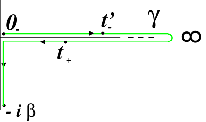
Figure 1: The Keldysh contour, starting at $t=0$, and ending at $t=-i\beta$, with $t$ on the backward branch and $t^{\prime}$ on the forward branch. By definition, any point lying on the vertical track is later than a point lying on the forward or backward branch.

If $z$ lies on the vertical track, then there is no need to extend the contour along the real axis. Instead, we have

$$O(z)=\frac{{\rm Tr}\,\left[e^{\beta\mu\hat{N}}e^{-i\int_{z}^{-i\beta}\mathrm{d}\bar{z}\hat{H}_{0}}\hat{O}e^{-i\int_{0}^{z}\mathrm{d}\bar{z}\hat{H}_{0}}\right]}{{\rm Tr}\,\left[e^{-\beta(\hat{H}_{0}-\mu\hat{N})}\right]}=\frac{{\rm Tr}\,\left[e^{-\beta(\hat{H}_{0}-\mu\hat{N})}\hat{O}\right]}{{\rm Tr}\,\left[e^{-\beta(\hat{H}_{0}-\mu\hat{N})}\right]},$$

where the cyclic property of the trace has been used. The right hand side is independent of $z$ and coincides with the thermal average ${\rm Tr}\,\{\hat{\rho}_{0}\hat{O}\}$. It is easy to verify that (5) would give exactly the same result for $O(t)$, where $t$ is real, if the Hamiltonian was time-independent, i.e. $\hat{H}(t)=\hat{H}_{0}$ also for $t>0$.

To summarize, in (5) the variable $z$ lies on the contour of Fig. 1; the r.h.s. gives the time-dependent statistical average of the observable $O$ when $z$ lies on the forward or backward branch, and the statistical average before the system is disturbed when $z$ lies on the vertical track.

III Nonequilibrium Green Functions

We now introduce the nonequilibrium Green function (NEGF), which is a function of two contour time-variables. In order to keep the notation as light as possible, we here discard the spin degree of freedom; the spin index may be restored later as needed. The field operators $\hat{\psi}(\vec{r})$, $\hat{\psi}^{{\dagger}}(\vec{r})$ destroy and create an electron in $\vec{r}$ and obey the anticommutation relations $\{\hat{\psi}(\vec{r}),\hat{\psi}^{{\dagger}}(\vec{r}^{\prime})\}=\delta(\vec{r}-\vec{r}^{\prime})$. We write the Hamiltonian $\hat{H}(t)$ as the sum of a quadratic term

$$\hat{h}(t)=\int\mathrm{d}\vec{r}\mathrm{d}\vec{r}^{\prime}\;\hat{\psi}^{{\dagger}}(\vec{r})\langle\vec{r}|\mathbf{h}(t)|\vec{r}^{\prime}\rangle\hat{\psi}(\vec{r}^{\prime})$$ (6)

and the interaction operator

$$\hat{H}_{w}=\frac{1}{2}\int\mathrm{d}\vec{r}\mathrm{d}\vec{r}^{\prime}\;\hat{\psi}^{{\dagger}}(\vec{r})\hat{\psi}^{{\dagger}}(\vec{r}^{\prime})w(\vec{r},\vec{r}^{\prime})\hat{\psi}(\vec{r}^{\prime})\hat{\psi}(\vec{r}).$$ (7)

We use boldface to indicate matrices in one-electron labels, e.g., $\mathbf{h}$ is a matrix and $\langle\vec{r}|\mathbf{h}|\vec{r}^{\prime}\rangle$ is the $(\vec{r},\vec{r}^{\prime})$ matrix element of $\mathbf{h}$. When describing electrons in an electro-magnetic field, the quadratic term is given by $\langle\vec{r}|\mathbf{h}(t)|\vec{r}^{\prime}\rangle=\delta(\vec{r}-\vec{r}^{\prime})\left\{[\nabla/i+\vec{A}(\vec{r},t)]^{2}/2+v(\vec{r},t)\right\}$.

The definition of an expectation value in (1) can be generalized to the expectation value of two operators. The Green function is defined as

$$G(\vec{r},z;\vec{r}^{\prime},z^{\prime})=\langle\vec{r}|\mathbf{G}(z;z^{\prime})|\vec{r}^{\prime}\rangle\equiv-i\langle T_{\mathrm{c}}[\hat{\psi}_{H}(\vec{r},z)\hat{\psi}_{H}^{{\dagger}}(\vec{r}^{\prime},z^{\prime})]\rangle,$$ (8)

where the contour variable in the field operators specifies the position in the contour ordering. The operators have a time-dependence according to the definition of the Heisenberg picture, e.g. $\hat{\psi}_{H}^{{\dagger}}(\vec{r},z)=\hat{S}(0;z)\hat{\psi}^{{\dagger}}(\vec{r})\hat{S}(z;0)$. Notice that if the time-argument $z$ is located on the real axis, then $\hat{\psi}_{H}(\vec{r},t_{+})=\hat{\psi}_{H}(\vec{r},t_{-})$. If the time-argument is on the imaginary axis, then $\hat{\psi}(\vec{r},-i\tau)$ is not the adjoint of $\hat{\psi}(\vec{r},-i\tau)$ since $\hat{S}^{\dagger}(-i\tau;0)\neq\hat{S}(0;-i\tau)$. The Green function can be written

$$\mathbf{G}(z;z^{\prime})=\theta(z,z^{\prime})\mathbf{G}^{>}(z;z^{\prime})+\theta(z^{\prime},z)\mathbf{G}^{<}(z;z^{\prime}).$$ (9)

The function $\theta(z,z^{\prime})$ is defined to be 1 if $z$ is later on the contour than $z^{\prime}$, and 0 otherwise. From the definition of the time-dependent expectation value in Eq. (4), it follows that the greater Green function $\mathbf{G}^{>}(z;z^{\prime})$, where $z$ is later on the contour than $z^{\prime}$, is

$$G^{>}(\vec{r},z;\vec{r}^{\prime},z^{\prime})=\frac{1}{i}\frac{{\rm Tr}\,\left[e^{\beta\mu\hat{N}}\hat{S}(-i\beta;0)\hat{\psi}_{H}(\vec{r},z)\hat{\psi}^{{\dagger}}_{H}(\vec{r}^{\prime},z^{\prime})\right]}{{\rm Tr}\,\left[e^{\beta\mu\hat{N}}\hat{S}(-i\beta;0)\right]}.$$ (10)

If $z^{\prime}$ is later on the contour than $z$, then the Green function equals

$$G^{<}(\vec{r},z;\vec{r}^{\prime},z^{\prime})=-\frac{1}{i}\frac{{\rm Tr}\,\left[e^{\beta\mu\hat{N}}\hat{S}(-i\beta;0)\hat{\psi}^{{\dagger}}_{H}(\vec{r}^{\prime},z^{\prime})\hat{\psi}_{H}(\vec{r},z)\right]}{{\rm Tr}\,\left[e^{\beta\mu\hat{N}}\hat{S}(-i\beta;0)\right]}.$$ (11)

The extra minus sign on the right hand side comes from the contour ordering. More generally, rearranging the field operators $\hat{\psi}$ and $\hat{\psi}^{{\dagger}}$ (later arguments to the left), we also have to multiply by $(-1)^{P}$, where $P$ is the parity of the permutation. From the definition of the Green function, it is easily seen that the electron density, $n(\vec{r},z)=\langle\hat{\psi}_{H}^{{\dagger}}(\vec{r},z)\hat{\psi}_{H}(\vec{r},z)\rangle$ and current is obtained according to

$$n(\vec{r},z)=-iG(\vec{r},z;\vec{r},z^{+})$$ (12)

$$\vec{j}(\vec{r},z)=-i\left\{\left[\frac{\nabla}{2i}-\frac{\nabla^{\prime}}{2i}+\vec{A}(\vec{r},z)\right]G(\vec{r},z;\vec{r}^{\prime},z^{\prime})\right\}_{z^{\prime}=z^{+}}.$$ (13)

where $z^{+}$ indicates that this time-argument is infinitesimally later on the contour.

The Green function $\mathbf{G}(z;z^{\prime})$ obeys an important cyclic relation on the Keldysh contour. Choosing $z=0_{-}$, which is the earliest time on the contour, we find $\mathbf{G}(0_{-};z^{\prime})=\mathbf{G}^{<}(0;z^{\prime})$, given by (11) with $\hat{\psi}_{H}(\vec{r},0)=\hat{\psi}(\vec{r})$. Inside the trace we can move $\hat{\psi}(\vec{r})$ to the left. Furthermore, we can exchange the position of $\hat{\psi}(\vec{r})$ and $e^{\beta\mu\hat{N}}$ by noting that $\hat{\psi}(\vec{r})e^{\beta\mu\hat{N}}=e^{\beta\mu(\hat{N}+1)}\hat{\psi}(\vec{r})$. Using the group identity $\hat{S}(-i\beta;0)\hat{S}(0;-i\beta)=1$, we obtain

$$G(\vec{r},0_{-};\vec{r}^{\prime},z^{\prime}) = -\frac{1}{i}\frac{{\rm Tr}\,\left[\hat{\psi}_{H}(\vec{r})e^{\beta\mu\hat{N}}\hat{S}(-i\beta;0)\hat{\psi}_{H}^{{\dagger}}(\vec{r}^{\prime},z^{\prime})\right]}{{\rm Tr}\,\left[e^{\beta\mu\hat{N}}\hat{S}(-i\beta;0)\right]}.$$ (14)

$$= -\frac{e^{\beta\mu}}{i}\frac{{\rm Tr}\,\left[e^{\beta\mu\hat{N}}\hat{S}(-i\beta;0)\hat{\psi}_{H}(\vec{r},-i\beta)\hat{\psi}_{H}^{{\dagger}}(\vec{r}^{\prime},z^{\prime})\right]}{{\rm Tr}\,\left[e^{\beta\mu\hat{N}}\hat{S}(-i\beta;0)\right]}.$$

The r.h.s. equals $-e^{\beta\mu}\langle\vec{r}|\mathbf{G}(-i\beta;z^{\prime})|\vec{r}^{\prime}\rangle$. Together with a similar analysis for $\mathbf{G}(z;0_{-})$, we conclude that

$$\mathbf{G}(0_{-};z^{\prime})=-e^{\beta\mu}\mathbf{G}(-i\beta;z^{\prime})\quad\mbox{and}\quad\mathbf{G}(z;0_{-})=-e^{-\beta\mu}\mathbf{G}(z;-i\beta).$$ (15)

These equations constitute the so called Kubo-Martin-Schwinger (KMS) boundary conditions kubo ; martin . From the definition of the Green function in (8), it is easily seen that the $\mathbf{G}(z;z)$ has a discontinuity in $z=z^{\prime}$,

$$\mathbf{G}^{>}(z;z)=\mathbf{G}^{<}(z;z)-i\mathbf{1}.$$ (16)

Furthermore, for both time-arguments on the real axis we have the important symmetry $\left[\mathbf{G}^{\lessgtr}(t^{\prime};t)\right]^{\dagger}=-\mathbf{G}^{\lessgtr}(t;t^{\prime})$. As we shall see, these relations play a crucial role in solving the equation of motion.

IV The Keldysh Book-Keeping

The Green function belongs to a larger class of functions of two time-contour variables that we will refer to as Keldysh space. These functions can be written on the form

$$k(z;z^{\prime})=\delta(z,z^{\prime})k^{\delta}(z)+\theta(z,z^{\prime})k^{>}(z;z^{\prime})+\theta(z^{\prime},z)k^{<}(z;z^{\prime}),$$ (17)

where the $\delta$-function on the contour is defined as $\delta(z,z^{\prime})=\mathrm{d}\theta(z,z^{\prime})/\mathrm{d}z$ . These functions are somewhat complicated due to the fact that each of the time-arguments can be located on three different brances of the contour, as illustrated in Fig. 1. Below we systematically derive a set of identities that are commonly used for dealing with such functions and will be used extensively in the following sections. Most of the relations are well known langreth , while others, equally important wagner , are not. Our aim is to provide a self-contained derivation of all of them. A table at the end of the Section summarizes the main results. For those who are not familiar with the Keldysh contour, we strongly recommend to scan what follows with pencil and paper.

It is straightforward to show that if $a(z;z^{\prime})$ and $b(z;z^{\prime})$ belong to the Keldysh space, then

$$c(z;z^{\prime})=\int_{\gamma}\mathrm{d}\bar{z}\;a(z;\bar{z})b(\bar{z};z^{\prime})$$ (18)

also belongs to the Keldysh space. For any $k(z;z^{\prime})$ in the Keldysh space we define the greater and lesser functions on the physical time axis

$$k^{>}(t;t^{\prime})\equiv k(t_{+};t^{\prime}_{-}),\quad k^{<}(t,t^{\prime})\equiv k(t_{-};t^{\prime}_{+}).$$

We also define the following two-point functions with one argument $t$ on the physical time axis and the other $\tau$ on the vertical track

$$k^{\rceil}(t;\tau)\equiv k(t_{\pm};\tau),\quad k^{\lceil}(\tau,t)\equiv k(\tau;t_{\pm}).$$ (19)

In the definition of $k^{\rceil}$ and $k^{\lceil}$ we can arbitrarily choose $t_{+}$ or $t_{-}$ since $\tau$ is later than both of them. The symbols “$\rceil$” and “$\lceil$” have been chosen in order to help the visualization of the time arguments. For instance, “$\rceil$” has a horizontal segment followed by a vertical one; correspondingly, $k^{\rceil}$ has a first argument which is real (and thus lies on the horizontal axis) and a second argument which is imaginary (and thus lies on the vertical axis). We will also use the convention of denoting the real time with latin letters and the imaginary time with greek letters.

If we write out the contour integral in (18) in detail, we see with the help of Fig. 1 that the integral consists of four main parts. First, we must integrate along the real axis from $\bar{z}=0_{-}$ to $\bar{z}=t^{\prime}_{-}$, for which $a=a^{>}$ and $b=b^{<}$. Then, the integral goes from $\bar{z}=t^{\prime}_{-}$ to $\bar{z}=t_{+}$, where $a=a^{>}$ and $b=b^{>}$. The third part of the integral goes along the real axis from $\bar{z}=t_{+}$ to $\bar{z}=0_{+}$, with $a=a^{<}$ and $b=b^{>}$. The last integral is along the imaginary track, from $0_{+}$ to $-i\beta$, where $a=a^{\rceil}$ and $b=b^{\lceil}$. In addition, we have the contribution from the singular parts, $a^{\delta}$ and $b^{\delta}$, which is trivial since these integrals involve a $\delta$-function. With these specifications, we can drop the $\pm$-subscripts on the time-arguments and write

$$c^{>}(t;t^{\prime}) = a^{>}(t,t^{\prime})b^{\delta}(t^{\prime})+a^{\delta}(t)b^{>}(t,t^{\prime})+\int_{0}^{t^{\prime}}\mathrm{d}\bar{t}\;a^{>}(t;\bar{t})b^{<}(\bar{t};t^{\prime})$$

$$+\int_{t^{\prime}}^{t}\mathrm{d}\bar{t}\;a^{>}(t;\bar{t})b^{>}(\bar{t};t^{\prime})+\int_{t}^{0}\mathrm{d}\bar{t}\;a^{<}(t;\bar{t})b^{>}(\bar{t};t^{\prime})+\int_{0}^{-i\beta}\mathrm{d}\bar{\tau}\;a^{\rceil}(t;\bar{\tau})b^{\lceil}(\bar{\tau};t^{\prime}).$$

The second integral on the r.h.s. is an ordinary integral on the real axis of two well defined functions and may be rewritten as

$$\int_{t^{\prime}}^{t}\mathrm{d}\bar{t}\;a^{>}(t;\bar{t})b^{>}(\bar{t};t^{\prime})=\int_{t^{\prime}}^{0}\mathrm{d}\bar{t}\;a^{>}(t;\bar{t})b^{>}(\bar{t};t^{\prime})+\int_{0}^{t}\mathrm{d}\bar{t}\;a^{>}(t;\bar{t})b^{>}(\bar{t};t^{\prime}).$$

Using this relation, the expression for $c^{>}$ becomes

$$c^{>}(t;t^{\prime}) = a^{>}(t,t^{\prime})b^{\delta}(t^{\prime})+a^{\delta}(t)b^{>}(t,t^{\prime})-\int_{0}^{t^{\prime}}\mathrm{d}\bar{t}\;a^{>}(t;\bar{t})[b^{>}(\bar{t};t^{\prime})-b^{<}(\bar{t};t^{\prime})]$$ (20)

$$+ \int_{0}^{t}\mathrm{d}\bar{t}\;[a^{>}(t;\bar{t})-a^{<}(t;\bar{t})]b^{>}(\bar{t};t^{\prime})+\int_{0}^{-i\beta}\mathrm{d}\bar{\tau}\;a^{\rceil}(t;\bar{\tau})b^{\lceil}(\bar{\tau};t^{\prime}).$$

Next, we introduce two other functions on the physical time axis

$$k^{\mathrm{R}}(t;t^{\prime}) \equiv \delta(t,t^{\prime})k^{\delta}+\theta(t-t^{\prime})[k^{>}(t;t^{\prime})-k^{<}(t;t^{\prime})],$$ (21)

$$k^{\mathrm{A}}(t;t^{\prime}) \equiv \delta(t,t^{\prime})k^{\delta}-\theta(t^{\prime}-t)[k^{>}(t;t^{\prime})-k^{<}(t;t^{\prime})].$$ (22)

The retarded function $k^{\mathrm{R}}(t;t^{\prime})$ vanishes for $t<t^{\prime}$, while the advanced function $k^{\mathrm{A}}(t;t^{\prime})$ vanishes for $t>t^{\prime}$. The retarded and advanced functions can be used to rewrite (20) in a more compact form

$$c^{>}(t;t^{\prime})=\int_{0}^{\infty}\mathrm{d}\bar{t}\,[a^{>}(t;\bar{t})b^{\mathrm{A}}(\bar{t};t^{\prime})+a^{\mathrm{R}}(t;\bar{t})b^{>}(\bar{t};t^{\prime})]+\int_{0}^{-i\beta}\mathrm{d}\bar{\tau}\,a^{\rceil}(t;\bar{\tau})b^{\lceil}(\bar{\tau};t^{\prime}).$$

It is convenient to introduce a short hand notation for integrals along the physical time axis and for those between 0 and $-i\beta$. The symbol “$\cdot$” will be used to write $\int_{0}^{\infty}\mathrm{d}\bar{t}f(\bar{t})g(\bar{t})$ as $f\cdot g$, while the symbol “$\star$” will be used to write $\int_{0}^{-i\beta}\mathrm{d}\bar{\tau}f(\bar{\tau})g(\bar{\tau})$ as $f\star g$. Then

$$c^{>}=a^{>}\cdot b^{\mathrm{A}}+a^{\mathrm{R}}\cdot b^{>}+a^{\rceil}\star b^{\lceil}.$$ (23)

Similarly, one can prove that

$$c^{<}=a^{<}\cdot b^{\mathrm{A}}+a^{\mathrm{R}}\cdot b^{<}+a^{\rceil}\star b^{\lceil}.$$ (24)

Equations (23-24) can be used to extract the retarded and advanced component of $c$. By definition

$$c^{\mathrm{R}}(t;t^{\prime}) = \delta(t-t^{\prime})c^{\delta}(t)+\theta(t-t^{\prime})[c^{>}(t;t^{\prime})-c^{<}(t;t^{\prime})]$$

$$= a^{\delta}(t)b^{\delta}(t^{\prime})\delta(t-t^{\prime})+\theta(t-t^{\prime})\int_{0}^{\infty}\mathrm{d}\bar{t}\,a^{\mathrm{R}}(t;\bar{t})[b^{>}(\bar{t};t^{\prime})-b^{<}(\bar{t};t^{\prime})]$$

$$+\theta(t-t^{\prime})\int_{0}^{\infty}\mathrm{d}\bar{t}\,[a^{>}(t;\bar{t})-a^{<}(t;\bar{t})]b^{\mathrm{A}}(\bar{t};t^{\prime}).$$

Using the definitions (21) and (22) to expand the integrals on the r.h.s. of this equation, it is straightforward to show that

$$c^{\mathrm{R}}=a^{\mathrm{R}}\cdot b^{\mathrm{R}}.$$ (25)

Proceeding along the same lines, one can show that the advanced component is given by $c^{\mathrm{A}}=a^{\mathrm{A}}\cdot b^{\mathrm{A}}$. It is worth noting that in the expressions for $c^{\mathrm{R}}$ and $c^{\mathrm{A}}$ no integration along the imaginary track is required.

Next, we show how to extract the components $c^{\rceil}$ and $c^{\lceil}$. We first define the Matzubara function $k^{\mathrm{M}}(\tau;\tau^{\prime})$ with both the arguments in the interval $(0,-i\beta)$:

$$k^{\mathrm{M}}(\tau;\tau^{\prime})\equiv k(z=\tau;z^{\prime}=\tau^{\prime}).$$

Let us focus on $k^{\rceil}$. Without any restrictions we may take $t_{-}$ as the first argument in (19). In this case, we find

$$c^{\rceil}(t;\tau)=a^{\delta}(t)b^{\rceil}(t;\tau)+\int_{0_{-}}^{t_{-}}\mathrm{d}\bar{z}a^{>}(t_{-};\bar{z})b^{<}(\bar{z};\tau)+\int_{t_{+}}^{0_{+}}\mathrm{d}\bar{z}a^{<}(t_{-};\bar{z})b^{<}(\bar{z};\tau)+\int_{0_{+}}^{-i\beta}\;\mathrm{d}\bar{z}\;a^{<}(t_{-};\bar{z})b(\bar{z};\tau).$$ (26)

Converting the contour integrals in integrals along the real time axis and along the imaginary track, and taking into account the definition in (21)

$$c^{\rceil}=a^{\mathrm{R}}\cdot b^{\rceil}+a^{\rceil}\star b^{\mathrm{M}}.$$ (27)

The relation for $c^{\lceil}$ can be obtained in a similar way and reads $c^{\lceil}=a^{\lceil}\cdot b^{\mathrm{A}}+a^{\mathrm{M}}\star b^{\lceil}$. Finally, it is straightforward to prove that the Matzubara component of $c$ is simply given by $c^{\mathrm{M}}=a^{\mathrm{M}}\star b^{\mathrm{M}}$.

There is another class of identities we want to discuss for completeness. We have seen that the convolution (18) of two functions belonging to the Keldysh space also belongs to the Keldysh space. The same holds true for the product

$$c(z;z^{\prime})=a(z;z^{\prime})b(z^{\prime};z).$$

Omitting the arguments of the functions, one readily finds (for $z\neq z^{\prime}$)

$$c^{>}=a^{>}b^{<},\;\;\;c^{<}=a^{<}b^{>},\quad c^{\rceil}=a^{\rceil}b^{\lceil},\;\;\;c^{\lceil}=a^{\lceil}b^{\rceil},\quad c^{\mathrm{M}}=a^{\mathrm{M}}b^{\mathrm{M}}.$$ (28)

The retarded function is then obtained exploiting the identities in (28). We have (for $t\neq t^{\prime}$)

$$c^{\mathrm{R}}(t;t^{\prime})=\theta(t-t^{\prime})[a^{>}(t;t^{\prime})b^{<}(t^{\prime};t)-a^{<}(t;t^{\prime})b^{>}(t^{\prime};t)].$$

We may get rid of the $\theta$-function by adding and subtracting $a^{<}b^{<}$ or $a^{>}b^{>}$ to the above relation and rearranging the terms. The final result is

$$c^{\mathrm{R}}=a^{\mathrm{R}}b^{<}+a^{<}b^{\mathrm{A}}=a^{\mathrm{R}}b^{>}+a^{>}b^{\mathrm{A}}.$$

Similarly one finds $c^{\mathrm{A}}=a^{\mathrm{A}}b^{<}+a^{<}b^{\mathrm{R}}=a^{\mathrm{A}}b^{>}+a^{>}b^{\mathrm{R}}$. The time-ordered and anti-time-ordered functions can be obtained in a similar way and the reader can look at Table 1 for the complete list of definitions and identities.

For later purposes, we also consider the case of a Keldysh function $k(z;z^{\prime})$ multiplied on the left by a scalar function $l(z)$. The scalar function is equivalent to the singular part of a function belonging to Keldysh space, $\tilde{l}(z;z^{\prime})=l(z)\delta(z,z^{\prime})$, meaning that $\tilde{l}^{\mathrm{R}/\mathrm{A}}=\tilde{l}^{\mathrm{M}}=\tilde{l}$ and $\tilde{l}^{\lessgtr}=\tilde{l}^{\rceil}=\tilde{l}^{\lceil}=0$. Using Table 1, one immediately realizes that the function $l$ is simply a prefactor: $\int_{\gamma}d\bar{z}\,\tilde{l}(z;\bar{z})k^{\mathrm{x}}(\bar{z};z^{\prime})=l(z)k^{\mathrm{x}}(z;z^{\prime})$, where $\mathrm{x}$ is one of the Keldysh components ($\lessgtr$, $\mathrm{R,\;A}$, $\rceil,\;\lceil$, $\mathrm{M}$). The same is true for $\int_{\gamma}\,k^{\mathrm{x}}(z;\bar{z})\tilde{r}(\bar{z};z^{\prime})=k^{\mathrm{x}}(z;z^{\prime})r(z^{\prime})$, where $\tilde{r}(z;z^{\prime})=r(z)\delta(z,z^{\prime})$ and $r(z)$ is a scalar function.

Table 1: Table of definitions of Keldysh functions and identities for the convolution and the product of two functions in the Keldysh space.

Definition	$c(z;z^{\prime})=\int_{\gamma}\mathrm{d}\bar{z}\;a(z;\bar{z})b(\bar{z};z^{\prime})$	$c(z;z^{\prime})=a(z;z^{\prime})b(z^{\prime};z)$
$k^{>}(t;t^{\prime})=k(t_{+};t^{\prime}_{-})$	$c^{>}=a^{>}\cdot b^{\mathrm{A}}+a^{\mathrm{R}}\cdot b^{>}+a^{\rceil}\star b^{\lceil}$	$c^{>}=a^{>}b^{<}$
$k^{<}(t;t^{\prime})=k(t_{-};t^{\prime}_{+})$	$c^{<}=a^{<}\cdot b^{\mathrm{A}}+a^{\mathrm{R}}\cdot b^{<}+a^{\rceil}\star b^{\lceil}$	$c^{<}=a^{<}b^{>}$
$\begin{array}[]{l}k^{\mathrm{R}}(t;t^{\prime})=\delta(t-t^{\prime})k^{\delta}(t)\\ \hskip 28.45274pt+\theta(t-t^{\prime})[k^{>}(t;t^{\prime})-k^{<}(t;t^{\prime})]\end{array}$	$c^{\mathrm{R}}=a^{\mathrm{R}}\cdot b^{\mathrm{R}}$	$c^{\mathrm{R}}=\left\{\begin{array}[]{l}a^{\mathrm{R}}b^{<}+a^{<}b^{\mathrm{A}}\\ a^{\mathrm{R}}b^{>}+a^{>}b^{\mathrm{A}}\end{array}\right.$
$\begin{array}[]{l}k^{\mathrm{A}}(t;t^{\prime})=\delta(t-t^{\prime})k^{\delta}(t)\\ \hskip 28.45274pt-\theta(t^{\prime}-t)[k^{>}(t;t^{\prime})-k^{<}(t;t^{\prime})]\end{array}$	$c^{\mathrm{A}}=a^{\mathrm{A}}\cdot b^{\mathrm{A}}$	$c^{\mathrm{A}}=\left\{\begin{array}[]{l}a^{\mathrm{A}}b^{<}+a^{<}b^{\mathrm{R}}\\ a^{\mathrm{A}}b^{>}+a^{>}b^{\mathrm{R}}\end{array}\right.$
$k^{\rceil}(t;\tau)=k(t_{\pm};\tau)$	$c^{\rceil}=a^{\mathrm{R}}\cdot b^{\rceil}+a^{\rceil}\star b^{\mathrm{M}}$	$c^{\rceil}=a^{\rceil}b^{\lceil}$
$k^{\lceil}(\tau,t)=k(\tau;t_{\pm})$	$c^{\lceil}=a^{\lceil}\cdot b^{\mathrm{A}}+a^{\mathrm{M}}\star b^{\lceil}$	$c^{\lceil}=a^{\lceil}b^{\rceil}$
$k^{\mathrm{M}}(\tau;\tau^{\prime})=k(z=\tau;z^{\prime}=\tau^{\prime})$	$c^{\mathrm{M}}=a^{\mathrm{M}}\star b^{\mathrm{M}}$	$c^{\mathrm{M}}=a^{\mathrm{M}}b^{\mathrm{M}}$

V The Kadanoff-Baym equations

The Green function, as defined in (9), satisfies the equation of motion

$$i\frac{\mathrm{d}}{\mathrm{d}z}\mathbf{G}(z;z^{\prime})={\bf 1}\delta(z,z^{\prime})+\mathbf{h}(z)\mathbf{G}(z;z^{\prime})+\int_{\gamma}d\bar{z}\,\mathbf{\Sigma}(z,\bar{z})\mathbf{G}(\bar{z};z^{\prime}),$$ (29)

as well as the adjoint equation

$$-i\frac{\mathrm{d}}{\mathrm{d}z^{\prime}}\mathbf{G}(z;z^{\prime})={\bf 1}\delta(z,z^{\prime})+\mathbf{G}(z;z^{\prime})\mathbf{h}(z^{\prime})+\int_{\gamma}d\bar{z}\,\mathbf{G}(z;\bar{z})\mathbf{\Sigma}(\bar{z},z^{\prime}).$$ (30)

The external potential is included in $\mathbf{h}$, while the self-energy $\mathbf{\Sigma}$ is a functional of the Green function, and describes the effects of the electron interaction. The self-energy belongs to Keldysh space and can therefore be written on the form $\mathbf{\Sigma}(z,z^{\prime})=\delta(z,z^{\prime})\mathbf{\Sigma}^{\delta}(z)+\theta(z,z^{\prime})\mathbf{\Sigma}^{>}(z,z^{\prime})+\theta(z^{\prime},z)\mathbf{\Sigma}^{<}(z,z^{\prime})$. The singular part of the self-energy can be identified as the Hartree–Fock potential, $\mathbf{\Sigma}^{\delta}(z)=\mathbf{v}_{\mathrm{H}}(z)+\mathbf{\Sigma}_{\mathrm{x}}(z)$. The self-energy obeys the same anti-periodic boundary conditions at $z=0_{-}$ and $z=-i\beta$ as $\mathbf{G}$. We will discuss self-energy approximations in more detail below.

Calculating the Green function on the time-contour now consists of two steps: 1) First one has to find the Green function for imaginary times, which is equivalent to finding the equilibrium Matzubara Green function $\mathbf{G}^{\mathrm{M}}(\tau,\tau^{\prime})$. This Green function depends only on the difference between the time-coordinates, and satisfies the KMS boundary conditions according to $\mathbf{G}^{\mathrm{M}}(\tau+i\beta,\tau^{\prime})=-e^{\beta\mu N}\mathbf{G}^{\mathrm{M}}(\tau,\tau^{\prime})$. Since the self-energy depends on the Green function, this amounts to solving the finite-temperature Dyson equation to self-consistency. 2) The Green function with one or two time-variables on the real axis can now be found by propagating according to (29) and (30). Starting from $t=0$, this procedure corresponds to extending the time-contour along the real time-axis. The process is illustrated in Fig. 2.

Figure 2: Propagating the Kadanoff-Baym equations means that one first determines the Green function for time-variables along the imaginary track. One then calculates the Green function with one or two variables on an expanding time-contour.

Writing out the equations for the components of $\mathbf{G}$ using Table 1, we obtain the equations known as the Kadanoff-Baym equations kb-book ,

$$i\frac{\mathrm{d}}{\mathrm{d}t}\mathbf{G}^{\lessgtr}(t;t^{\prime})=\mathbf{h}(t)\mathbf{G}^{\lessgtr}(t;t^{\prime})+\left[\mathbf{\Sigma}^{\mathrm{R}}\cdot\mathbf{G}^{\lessgtr}\right](t;t^{\prime})+\left[\mathbf{\Sigma}^{\lessgtr}\cdot\mathbf{G}^{\mathrm{A}}\right](t;t^{\prime})+\left[\mathbf{\Sigma}^{\rceil}\star\mathbf{G}^{\lceil}\right](t,t^{\prime}),$$ (31)

$$-i\frac{\mathrm{d}}{\mathrm{d}t^{\prime}}\mathbf{G}^{\lessgtr}(t;t^{\prime})=\mathbf{G}^{\lessgtr}(t;t^{\prime})\mathbf{h}(t^{\prime})+\left[\mathbf{G}^{\lessgtr}\cdot\mathbf{\Sigma}^{\mathrm{A}}\right](t;t^{\prime})+\left[\mathbf{G}^{\mathrm{R}}\cdot\mathbf{\Sigma}^{\lessgtr}\right](t;t^{\prime})+\left[\mathbf{G}^{\rceil}\star\mathbf{\Sigma}^{\lceil}\right](t,t^{\prime}),$$ (32)

$$i\frac{\mathrm{d}}{\mathrm{d}t}\mathbf{G}^{\rceil}(t;\tau)=\mathbf{h}(t)\mathbf{G}^{\rceil}(t;\tau)+\left[\mathbf{\Sigma}^{\mathrm{R}}\cdot\mathbf{G}^{\rceil}\right](t;\tau)+\left[\mathbf{\Sigma}^{\rceil}\star\mathbf{G}^{\mathrm{M}}\right](t,\tau),$$ (33)

and

$$-i\frac{\mathrm{d}}{\mathrm{d}t}\mathbf{G}^{\lceil}(\tau;t)=\mathbf{G}^{\lceil}(\tau;t)\mathbf{h}(t)+\left[\mathbf{\Sigma}^{\lceil}\cdot\mathbf{G}^{\mathrm{A}}\right](\tau,t)+\left[\mathbf{\Sigma}^{\mathrm{M}}\star\mathbf{G}^{\lceil}\right](\tau;t).$$ (34)

It is easily seen that if we denote by $T$ the largest of the two time-arguments $t$ and $t^{\prime}$, then the right hand sides of (31) and (32) depend on $\mathbf{G}^{\lessgtr}(t_{1};t_{2})$, $\mathbf{G}^{\lceil}(\tau_{1},t_{2})$ and $\mathbf{G}^{\rceil}(t_{1},\tau_{2})$ for $t_{1},t_{2}\leq T$. When propagating the Kadanoff-Baym equations one therefore starts at $t=t^{\prime}=0$, with the initial conditions given by $\mathbf{G}^{<}(0;0)=\lim_{\eta\to 0}\mathbf{G}^{\mathrm{M}}(0;-i\eta)$, $\mathbf{G}^{>}(0;0)=\lim_{\eta\to 0}\mathbf{G}^{\mathrm{M}}(-i\eta;0)$, $\mathbf{G}^{\lceil}(\tau,0)=\mathbf{G}^{M}(\tau,0)$ and $\mathbf{G}^{\rceil}(0,\tau)=\mathbf{G}^{M}(0,\tau)$. One then calculates $\mathbf{G}^{\lessgtr}(t,t^{\prime})$ for time-arguments within the expanding square given by $t,t^{\prime}\leq T$. Simultaneously, one calculates $\mathbf{G}^{\lceil}(t,\tau)$ and $\mathbf{G}^{\rceil}(\tau,t)$ for $t\leq T$. The resulting $\mathbf{G}$ then automatically satisfies the KMS boundary conditions. The Kadanoff-Baym equations (31) and (33) can both be written in the form

$$i\frac{\mathrm{d}}{\mathrm{d}t}\mathbf{G}^{\mathrm{x}}(t;z^{\prime})=\mathbf{h}^{\mathrm{HF}}(t)\mathbf{G}^{\mathrm{x}}(t;z^{\prime})+\mathbf{I}^{\mathrm{x}}(t;z^{\prime}),$$ (35)

while (32) and (34) can be written as the adjoint equations. The term proportional to $\mathbf{h}^{\mathrm{HF}}\equiv\mathbf{h}+\mathbf{\Sigma}^{\delta}$ describes a free-particle propagation, while $\mathbf{I}^{\mathrm{x}}$ is a collision term, which introduces memory effects and dissipation. As can be seen from (31–34), the only contribution to $\mathbf{I}^{\mathrm{x}}(0;0)$ comes from terms containing time-arguments on the imaginary axis. These terms therefore contain the effect of initial correlations, since the time-derivative of $\mathbf{G}$ would otherwise correspond to that of a non-interacting system, i.e., $\mathbf{I}^{\mathrm{x}}(0;0)=0$.

An example of a time-propagation is given in Fig. 3, which shows the Green function for an H₂ molecule. In this example, the Green function is represented in a basis of Hartree–Fock molecular orbitals, $\langle\vec{r}|\mathbf{G}(z,z^{\prime})|\vec{r}^{\prime}\rangle=\sum_{ij}\phi_{i}(\vec{r})G_{ij}(z,z^{\prime})\phi^{*}_{j}(\vec{r}^{\prime})$, where $\phi_{i}(\vec{r})=\langle\vec{r}|\phi_{i}\rangle$.

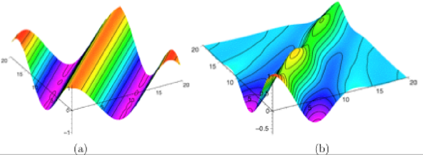
Figure 3: The figures show the Green function $\mathrm{Im}\,G^{<}_{\sigma_{g},\sigma_{g}}(t_{1},t_{2})$, where the matrix indices refer to the groundstate $\sigma_{g}$ Hartree–Fock orbital of the molecule. The figure on the left shows the system in equilibrium, while the system on the right has an additional electric field, $\theta(t)E_{0}z$. The times $t_{1}$ and $t_{2}$ on the axes are given in atomic units.

We have here propagated the Kadanoff-Baym equations using the second Born approximation, illustrated in Fig. 4b. The plots show the imaginary part of the matrix element $G^{<}_{\sigma_{g},\sigma_{g}}(t,t^{\prime})$ calculated for time-variables within the square $t_{1},t_{2}\leq T=20.0$ atomic units. In the plot to the left, there is no added external potential and the molecule remains in equilibrium. This means that the Green function only depends on the difference $t_{2}-t_{1}$, and the oscillations in this time-coordinate has a frequency given by the ionization potential of the molecule, in agreement with equilibrium Green function theory fetterwalecka . The figure on the right shows the same matrix element, but now in the presence of an additional electric field which is switched on at $t=0$. The oscillations along the ridge $t_{1}=t_{2}$ can be interpreted as oscillations in the occupation number.

VI Conserving approximations

In the Dyson-Schwinger equations (29) and (30), we introduced the electronic self-energy functional $\mathbf{\Sigma}$, which accounts for the effects of the electron interaction. The self-energy is a functional of the Green function, and will have to be approximated in practical calculations. Diagrammatic techniques provide a natural scheme for generating approximate self-energies and for systematically improving the approximations. There are no general prescriptions for how to select the relevant diagrams, which means that this selection must be guided by physical intuition. There are, however, important conservation laws, like the number conservation law or the energy conservation law, that should always be obeyed. We will in the following discuss an exact framework for generating such conserving approximations.

Let us first discuss the conservation laws obeyed by a system of interacting electrons, in an external field given by the electrostatic potential $v(\vec{r},t)$ and vector potential $\vec{A}(\vec{r},t)$. An important relation between these two quantities is provided by the continuity equation

$$\frac{\mathrm{d}}{\mathrm{d}t}n(\vec{r},t)+\nabla\cdot\vec{j}(\vec{r},t)=0.$$ (36)

The density and the current density can be calculated from the Green function using (12) and (13). Whether these quantities will agree with the continuity equation will depend on whether the Green function is obtained from a conserving self-energy approximation. If we know the current density we can also calculate the total momentum and angular momentum expectation values in the system from the equations

$$\vec{P}(t)=\int d\vec{r}\,\vec{j}(\vec{r},t)\\ \qquad\mbox{and}\qquad\vec{L}(t)=\int d\vec{r}\,\vec{r}\times\vec{j}(\vec{r},t).$$ (37)

For these two quantities the following relations should be satisfied

$$\frac{\mathrm{d}}{\mathrm{d}t}\vec{P}(t) = -\int d\vec{r}\Big{[}n(\vec{r},t)\,\vec{E}(\vec{r},t)+\vec{j}(\vec{r},t)\times\vec{B}(\vec{r},t)\Big{]}$$ (38)

$$\frac{\mathrm{d}}{\mathrm{d}t}\vec{L}(t) = -\int d\vec{r}\Big{[}n(\vec{r},t)\vec{r}\times\vec{E}(\vec{r},t)+\vec{r}\times(\vec{j}(\vec{r},t)\times\vec{B}(\vec{r},t))\Big{]}.$$ (39)

where $\vec{E}$ and $\vec{B}$ are the electric and magnetic fields calculated from

$$\vec{E}(\vec{r},t)=\nabla v(\vec{r},t)-\partial_{t}\vec{A}(\vec{r},t)\qquad\mbox{and}\qquad\vec{B}(\vec{r},t)=\nabla\times\vec{A}(\vec{r},t).$$ (40)

The equations (38) and (39) tell us that the change in momentum and angular momentum is equal to the total force and total torque on the system. In the absence of external fields these equations express momentum and angular momentum conservation. Since the right hand sides of (38) and (39) can also directly be calculated from the density and the current and therefore from the Green function, we may wonder whether they are satisfied for a given approximation to the Green function.

Finally we will consider the case of energy conservation. Let $E(t)=\langle\hat{H}(t)\rangle$ be the energy expectation value of the system, then we have

$$\frac{\mathrm{d}}{\mathrm{d}t}E(t)=-\int d\vec{r}\,\vec{j}(\vec{r},t)\cdot\vec{E}(\vec{r},t)$$ (41)

This equation tells us that the energy change of the system is equal to the work done on the system. The total energy is calculated from the Green function using the expression

$$E(t)=-\frac{i}{2}\int d\vec{r}\left.\langle\vec{r}|\left[i\frac{\mathrm{d}}{\mathrm{d}t}+\mathbf{h}(t)\right]\mathbf{G}^{<}(t,t^{\prime})|\vec{r}\rangle\right|_{t^{\prime}=t}.$$ (42)

The question is now whether the energy and the current calculated from an approximate Green function satisfy the relation in (41).

Baym and Kadanoff baym1 ; baym2 showed that conserving approximations follow immediately if the self-energy is obtained as the functional derivative,

$$\Sigma(1;2)=\frac{\delta\Phi}{\delta G(2;1)}.$$ (43)

Here, and in the following discussion, we use numbers to denote the contour coordinates, such that $1=(\vec{r}_{1},z_{1})$. A functional $\Phi$ can be constructed, as first shown in a seminal paper by Luttinger and Ward lw , by summing over irreducible self-energy diagrams closed with an additional Green function line and multiplied by appropriate numerical prefactors,

$$\Phi[G]=\sum_{n,k}\frac{1}{2n}\int d\bar{1}d\bar{2}\,\Sigma_{n}^{(k)}(\bar{1};\bar{2})G(\bar{2};\bar{1}).$$ (44)

In this summation, $\Sigma_{n}^{(k)}$ denotes a self-energy diagram of $n$-th order, i.e. containing $n$ interaction lines. The time-integrals go along the contour, but the rules for constructing Feynman diagrams are otherwise exactly the same as those in the ground-state formalism fetterwalecka . Notice that the functional derivative in (43) may generate other self-energy diagrams in addition to those used in the construction of $\Phi$ in (44).

Figure 4: Diagrams for the generating functional $\Phi$, and the corresponding self-energy diagrams. In (a) we have the exchange diagram, and (b) the second Born approximation. The diagrams in (c) and (d) belong to the $GW$ approximation and the $T$-matrix approximation respectively.

In Fig. 4 we show some examples of typical $\Phi$ diagrams. Examples of $\Phi$-derivable approximations include Hartree–Fock, the second Born approximation, the $GW$ approximation and the $T$-matrix approximation.

When the Green function is calculated from a conserving approximation, the resulting observables agree with the conservation laws of the underlying Hamiltonian, as given in (36), (38), (39), and (41). This guarantees the conservation of particles, energy, momentum, and angular momentum. All these conservation laws follow from the invariance of $\Phi$ under specific changes in $G$. We will here only outline the principles of the proofs, without going into the details, which can be found in baym1 ; baym2 . 1) Number conservation follows from the gauge invariance of $\Phi$. A gauge transformation $\vec{A}(1)\to\vec{A}(1)+\nabla\Lambda(1)$, where $\Lambda(\vec{r},0_{-})=\Lambda(\vec{r},-i\beta)$ leaves $\Phi$ unchanged. A consequence of the gauge invariance is that a pure gauge cannot induce a change in the density or current. The invariance is therefore closely related to the Ward-identities and to the $f$-sum rule for the density response function vanleeuwen04 . 2) Momentum conservation follows from the invariance of $\Phi$ under spatial translations, $\vec{r}\to\vec{r}+\vec{R}(z)$. The invariance is a consequence of the electron interaction $v(1,2)=\delta(z_{1},z_{2})/|\vec{r}_{1}-\vec{r}_{2}|$ being instantaneous and only depending on the difference between the spatial coordinates. 3) Angular momentum conservation follows from the invariance of $\Phi$ under a rotation of the spatial coordinates. 4) Energy conservation follows from the invariance of $\Phi$ when described by an observer using a ”rubbery clock”, measuring time according to the function $s(z)$. The invariance relies on the electron interaction being instantaneous.

VII Non-interacting Electrons

In this Section we focus on non-interacting electrons. This is particularly relevant for TDDFT, where the electrons are described by the non-interacting Kohn-Sham system. While the Kohn-Sham Green function differs from the true Green function, they both produce the same time-dependent density. This is important since the density is not only an important observable in, e.g., quantum transport, but also since the density is the central ingredient in TDDFT. The use of NEGFs in TDDFT is therefore important due to the relation between $v_{\mathrm{xc}}$ and the self-energy.

For a system of non-interacting electrons $\hat{H}_{v}=0$ and it is straightforward to show that the Green function obeys the equations of motion (29) and (30), with $\mathbf{\Sigma}=0$. For any $z\neq z^{\prime}$, the equations of motion can be solved by using the evolution operator on the contour,

$$\mathbf{S}(z,z^{\prime})=T_{\mathrm{c}}\left\{e^{-i\int_{z^{\prime}}^{z}\mathrm{d}\bar{z}\;\mathbf{h}(\bar{z})}\right\},$$

which solves $i\frac{\mathrm{d}}{\mathrm{d}z}\mathbf{S}(z,z^{\prime})=\mathbf{h}(z)\mathbf{S}(z,z^{\prime})$ and $-i\frac{\mathrm{d}}{\mathrm{d}z^{\prime}}\mathbf{S}(z,z^{\prime})=\mathbf{S}(z,z^{\prime})\mathbf{h}(z^{\prime})$. Therefore, any Green function

$$\mathbf{G}(z;z^{\prime})=\theta(z,z^{\prime})\mathbf{S}(z,0_{-})\vec{f}^{>}\mathbf{S}(0_{-},z^{\prime})+\theta(z^{\prime},z)\mathbf{S}(z,0_{-})\vec{f}^{<}\mathbf{S}(0_{-},z^{\prime}),$$ (45)

satisfying the constraint (16) on the form

$$\vec{f}^{>}-\vec{f}^{<}=-i{\bf 1},$$ (46)

is a solution of the (29-30). In order to fix the matrix $\vec{f}^{>}$ or $\vec{f}^{<}$ we impose the KMS boundary conditions. The matrix $\mathbf{h}(z)=\mathbf{h}_{0}$ for any $z$ on the vertical track, meaning that $\mathbf{S}(-i\beta,0_{-})=e^{-\beta\mathbf{h}_{0}}$. Equation (15) then implies $\vec{f}^{<}=-e^{-\beta(\mathbf{h}_{0}-\mu)}\vec{f}^{>}$, and taking into account the constraint (46) we conclude that

$$\vec{f}^{<}=\frac{i}{e^{\beta(\mathbf{h}_{0}-\mu)}+1}=if(\mathbf{h}_{0}),$$

where $f(\omega)=1/[e^{\beta(\omega-\mu)}+1]$ is the Fermi distribution function. The matrix $\vec{f}^{>}$ takes the form $\vec{f}^{>}=i[f(\mathbf{h}_{0})-{\bf 1}]$.

The Green function $\mathbf{G}(z;z^{\prime})$ for a system of non-interacting electrons is now completely fixed. Both $\mathbf{G}^{>}$ and $\mathbf{G}^{<}$ depend on the initial distribution function $f(\mathbf{h}_{0})$, as it should according to the discussion of Section III. Another way of writing $-i\mathbf{G}^{<}$ is in terms of the eigenstates $|\varphi_{n}\rangle\equiv|\varphi_{n}(0)\rangle$ of $\mathbf{h}_{0}$ with eigenvalues $\varepsilon_{n}$. From the time-evolved eigenstate $|\varphi_{n}(t)\rangle=\mathbf{S}(t,0)|\varphi_{n}\rangle$ we can calculate the time-dependent wavefunction $\varphi_{n}(\vec{r},t)=\langle\vec{r}|\varphi_{n}(t)\rangle$. Inserting $\sum_{n}|\varphi_{n}(0)\rangle\langle\varphi_{n}(0)|$ in the expression for $\mathbf{G}^{<}$ we find

$$-iG^{<}(\vec{r},t;\vec{r}^{\prime},t^{\prime})=-i\sum_{m,n}\langle\vec{r}|\mathbf{S}(t;0)|\varphi_{m}\rangle\langle\varphi_{m}|\vec{f}^{<}|\varphi_{n}\rangle\langle\varphi_{n}|\mathbf{S}(0;t)\vec{r}^{\prime}\rangle=\sum_{n}f(\varepsilon_{n})\varphi_{n}(\vec{r},t)\varphi_{n}^{\ast}(\vec{r}^{\prime},t^{\prime}),$$ (47)

which for $t=t^{\prime}$ reduces to the time-dependent density matrix. The Green function $\mathbf{G}^{>}$ becomes

$$-iG^{>}(\vec{r},t;\vec{r}^{\prime},t^{\prime})=-\sum_{n}[1-f(\varepsilon_{n})]\varphi_{n}(\vec{r},t)\varphi_{n}^{\ast}(\vec{r}^{\prime},t^{\prime}),$$ (48)

Knowing the greater and lesser Green functions we can also calculate $\mathbf{G}^{\mathrm{R},\mathrm{A}}$. By definition we have

$$\mathbf{G}^{\mathrm{R}}(t;t^{\prime})=\theta(t-t^{\prime})[\mathbf{G}^{>}(t;t^{\prime})-\mathbf{G}^{<}(t;t^{\prime})]=-i\theta(t-t^{\prime})\mathbf{S}(t,t^{\prime}),$$

and similarly

$$\mathbf{G}^{\mathrm{A}}(t;t^{\prime})=i\theta(t^{\prime}-t)\mathbf{S}(t,t^{\prime})=[\mathbf{G}^{\mathrm{R}}(t^{\prime};t)]^{{\dagger}}.$$ (49)

In the above expressions the Fermi distribution function has disappeared. The information carried by $\mathbf{G}^{\mathrm{R},\mathrm{A}}$ is the same contained in the one-particle evolution operator. There is no information on how the system is prepared (how many particles, how they are distributed, etc). We use this observation to rewrite $\mathbf{G}^{\lessgtr}$ in terms of $\mathbf{G}^{\mathrm{R},\mathrm{A}}$

$$\mathbf{G}^{\lessgtr}(t;t^{\prime})=\mathbf{G}^{\mathrm{R}}(t;0)\mathbf{G}^{\lessgtr}(0;0)\mathbf{G}^{\mathrm{A}}(0;t^{\prime}).$$ (50)

Thus, $\mathbf{G}^{\lessgtr}$ is completely known once we know how to propagate the one-electron orbitals in time and how they are populated before the system is perturbed blandin ; cini ; stefanucci . We also observe that an analogous relation holds for $\mathbf{G}^{\rceil,\lceil}$

$$\mathbf{G}^{\rceil}(t;\tau)=i\mathbf{G}^{\mathrm{R}}(t;0)\mathbf{G}^{\rceil}(0;\tau),\quad\mathbf{G}^{\lceil}(\tau;t)=-i\mathbf{G}^{\lceil}(\tau;0)\mathbf{G}^{\mathrm{A}}(0;\tau).$$

Let us now focus on a special kind of disturbance, namely $\mathbf{h}(t)=\mathbf{h}_{0}+\theta(t)\mathbf{h}_{1}$. In this case

$$\mathbf{G}^{\mathrm{R}}(t;t^{\prime})=-i\theta(t-t^{\prime})e^{-i(\mathbf{h}_{0}+\mathbf{h}_{1})(t-t^{\prime})}$$ (51)

depends only on the difference between the time arguments. Let us define the Fourier transform of $\mathbf{G}^{\mathrm{R},\mathrm{A}}$ from

$$\mathbf{G}^{\mathrm{R},\mathrm{A}}(t;t^{\prime})=\int\frac{\mathrm{d}\omega}{2\pi}e^{-i\omega(t-t^{\prime})}\mathbf{G}^{\mathrm{R},\mathrm{A}}(\omega).$$

The step function can be written as $\theta(t-t^{\prime})=\int\frac{\mathrm{d}\omega}{2\pi i}\frac{e^{i\omega(t-t^{\prime})}}{\omega-i\eta}$, with $\eta$ an infinitesimally small positive constant. Substituting this representation of the $\theta$-function into (51) and shifting the $\omega$ variable one readily finds

$$\mathbf{G}^{\mathrm{R}}(\omega)=\frac{1}{\omega-\mathbf{h}_{0}-\mathbf{h}_{1}+i\eta},$$

and therefore $\mathbf{G}^{\mathrm{R}}(\omega)$ is analytic in the upper half plane. On the other hand, from (49) it follows that $\mathbf{G}^{\mathrm{A}}(\omega)=[\mathbf{G}^{\mathrm{R}}(\omega)]^{{\dagger}}$ is analytic in the lower half plane. What can we say about the greater and lesser component? Do they also depend only on the difference $t-t^{\prime}$? The answer to the latter question is negative. Indeed, we recall that they contain information on how the system is prepared before $\mathbf{h}_{1}$ is switched on. In particular the original eigenstates are eigenstates of $\mathbf{h}_{0}$ and in general are not eigenstates of the Hamiltonian $\mathbf{h}_{0}+\mathbf{h}_{1}$ at positive times. From (50) one can see that $\mathbf{G}^{\lessgtr}(t;t^{\prime})$ cannot be expressed only in terms of the time difference $t-t^{\prime}$. For instance

$$\mathbf{G}^{<}(t;t^{\prime})=e^{-i(\mathbf{h}_{0}+\mathbf{h}_{1})t}if(\mathbf{h}_{0})e^{i(\mathbf{h}_{0}+\mathbf{h}_{1})t^{\prime}},$$

and unless $\mathbf{h}_{0}$ and $\mathbf{h}_{1}$ commute, it is a function of $t$ and $t^{\prime}$ separately.

It is sometimes useful to split $\mathbf{h}(t)$ in two parts and treat one of them perturbatively. Let us think, for instance, of a system composed of two connected subsystems $A+B$. In case we know how to calculate the Green function of the isolated subsystems $A$ and $B$, it is convenient to treat the connecting part as a perturbation. Thus, we write $\mathbf{h}(t)=\mbox{\boldmath${\cal E}$}(t)+\mbox{\boldmath${\cal V}$}(t)$, and we define $\mathbf{g}$ as the Green function when $\mbox{\boldmath${\cal V}$}=0$. The $\mathbf{g}$ is a solution of

$$\left\{i\frac{\mathrm{d}}{\mathrm{d}z}-\mbox{\boldmath${\cal E}$}(z)\right\}\mathbf{g}(z;z^{\prime})={\bf 1}\delta(z,z^{\prime}),$$

and of the corresponding adjoint equation of motion. Furthermore, the Green function $\mathbf{g}$ obeys the KMS boundary conditions. With these we can use $\mathbf{g}$ to convert the equations of motion for $\mathbf{G}$ into integral equations

$$\mathbf{G}(z;z^{\prime})=\mathbf{g}(z;z^{\prime})+\int_{\gamma}\mathrm{d}\bar{z}\;\mathbf{g}(z;\bar{z})\mbox{\boldmath${\cal V}$}(\bar{z})\mathbf{G}(\bar{z};z^{\prime})=\mathbf{g}(z;z^{\prime})+\int_{\gamma}\mathrm{d}\bar{z}\;\mathbf{G}(z;\bar{z})\mbox{\boldmath${\cal V}$}(\bar{z})\mathbf{g}(\bar{z};z^{\prime});$$ (52)

the integral on $\bar{z}$ is along the generalized Keldysh contour of Fig. 1. One can easily check that this $\mathbf{G}$ satisfies both (29) and (30). $\mathbf{G}$ also obeys the KMS boundary conditions since the integral equation is defined on the contour of Fig. 1.

In order to get some familiarity with the above perturbation scheme, we consider explicitly the system $A+B$ already mentioned. We partition the one-electron Hilbert space in states of the subsystem $A$ and states of the subsystem $B$. The “unperturbed” system is described by ${\cal E}$, while the connecting part by ${\cal V}$ and

$$\mbox{\boldmath${\cal E}$}=\left[\begin{array}[]{cc}\mbox{\boldmath${\cal E}$}_{AA}&0\\ 0&\mbox{\boldmath${\cal E}$}_{BB}\end{array}\right],\quad\quad\mbox{\boldmath${\cal V}$}=\left[\begin{array}[]{cc}0&\mbox{\boldmath${\cal V}$}_{AB}\\ \mbox{\boldmath${\cal V}$}_{BA}&0\end{array}\right].$$

Taking into account that $\mathbf{g}$ has no off-diagonal matrix elements, the Green function projected on one of the two subsystems, e.g., $\mathbf{G}_{BB}$, is

$$\mathbf{G}_{BB}(z;z^{\prime})=\mathbf{g}_{BB}(z;z^{\prime})+\int_{\gamma}\mathrm{d}\bar{z}\;\mathbf{g}_{BB}(z;\bar{z})\mbox{\boldmath${\cal V}$}_{BA}(\bar{z})\mathbf{G}_{AB}(\bar{z};z^{\prime})$$

and

$$\mathbf{G}_{AB}(z;z^{\prime})=\int_{\gamma}\mathrm{d}\bar{z}\;\mathbf{g}_{AA}(z;\bar{z})\mbox{\boldmath${\cal V}$}_{AB}(\bar{z})\mathbf{G}_{BB}(\bar{z};z^{\prime}).$$

Substituting this latter equation into the first one, we obtain a closed equation for $\mathbf{G}_{BB}$:

$$\mathbf{G}_{BB}(z;z^{\prime})=\mathbf{g}_{BB}(z;z^{\prime})+\int_{\gamma}\mathrm{d}\bar{z}\mathrm{d}\bar{z}^{\prime}\mathbf{g}_{BB}(z;\bar{z})\mathbf{\Sigma}_{BB}(\bar{z};\bar{z}^{\prime})\mathbf{G}_{BB}(\bar{z}^{\prime};z^{\prime}),$$ (53)

with

$$\mathbf{\Sigma}_{BB}(\bar{z};\bar{z}^{\prime})=\mbox{\boldmath${\cal V}$}_{BA}(\bar{z})\mathbf{g}_{AA}(\bar{z};\bar{z}^{\prime})\mbox{\boldmath${\cal V}$}_{AB}(\bar{z}^{\prime})$$

the embedding self-energy. The retarded and advanced component can now be easily computed. With the help of Table 1 one finds

$$\mathbf{G}_{BB}^{\mathrm{R},\mathrm{A}}=\mathbf{g}_{BB}^{\mathrm{R},\mathrm{A}}+\mathbf{g}^{\mathrm{R},\mathrm{A}}_{BB}\cdot\mathbf{\Sigma}^{\mathrm{R},\mathrm{A}}_{BB}\cdot\mathbf{G}^{\mathrm{R},\mathrm{A}}_{BB}.$$

Next, we have to compute the lesser or greater component. As for the retarded and advanced components, this can be done starting from (53). The reader can soon realize that the calculation is rather complicated, due to the mixing of pure real-time functions with function having one real time argument and one imaginary time argument, see Table 1. Below, we use (50) as a feasible short-cut. A closed equation for the retarded and advanced component has been already obtained. Thus, we simply need an equation for $\mathbf{G}^{\lessgtr}(0;0)$. Let us focus on the lesser component $\mathbf{G}^{<}(0;0)=i\vec{f}^{<}$. Assuming that the Hamiltonian $\mathbf{h}_{0}$ is hermitian, the matrix $(\omega-\mathbf{h}_{0})^{-1}$ has poles at frequencies equal to the eigenvalues of $\mathbf{h}_{0}$. These poles are all on the real frequency axis, and we can therefore write

$$\mathbf{G}^{<}(0;0)=if(\mathbf{h}_{0})=\int_{\gamma}\frac{d\zeta}{2\pi}f(\zeta)\frac{1}{\zeta-\mathbf{h}_{0}},$$ (54)

where the contour $\gamma$ encloses the real frequency axis.

VIII Action functional and TDDFT

We define the action functional

$$\tilde{A}=i\ln{\rm Tr}\,\left\{e^{\beta\mu\hat{N}}\hat{S}(-i\beta;0)\right\},$$ (55)

where the evolution operator $\hat{S}$ is the same as defined in (3). The action functional is a tool for generating equations of motion, and is not interesting per se. Nevertheless, one should notice that the action, as defined in (55) has a numerical value equal to $i\ln Z$, where $Z$ is the thermodynamic partition function.

It is easy to show that if we make a perturbation $\delta\hat{V}(z)$ in the Hamiltonian, the change in the evolution operator is given by

$$i\frac{\mathrm{d}}{\mathrm{d}z}\delta\hat{S}(z;z^{\prime})=\delta\hat{V}(z)\hat{S}(z;z^{\prime})+\hat{H}(z)\delta S(z;z^{\prime}).$$ (56)

A similar equation for the dependence on $z^{\prime}$, and the boundary condition $\delta\hat{S}(z;z)=0$ gives

$$\delta\hat{S}(z;z^{\prime})=-i\int_{z^{\prime}}^{z}d\bar{z}\,\hat{S}(z;\bar{z})\delta\hat{V}(\bar{z})\hat{S}(\bar{z},z^{\prime}).$$ (57)

We stress that the time-coordinates are on a contour going from $0$ to $-i\beta$. The variation in, e.g., $V(t_{+})$ is therefore independent of the variation in $V(t_{-})$. If we let $\delta\hat{V}(z)=\int d\vec{r}\,\delta v(\vec{r},z)\hat{n}(\vec{r})$, a combination of (55) and (57) yields [compare to (4)] the expectation values of the density,

$$\frac{\delta\tilde{A}}{\delta v(\vec{r},z)} = \frac{i}{{\rm Tr}\,\left\{e^{\beta\mu\hat{N}}\hat{S}(-i\beta;0)\right\}}\frac{\delta}{\delta v(\vec{r},z)}{\rm Tr}\,\left\{e^{\beta\mu N}\hat{S}(-i\beta;0)\right\}$$ (58)

$$= \frac{{\rm Tr}\,\left\{e^{\beta\mu\hat{N}}\hat{S}(-i\beta;0)\hat{S}(0;z)\hat{n}(\vec{r})\hat{S}(z,0)\right\}}{{\rm Tr}\,\left\{e^{\beta\mu\hat{N}}\hat{S}(-i\beta;0)\right\}}=n(\vec{r},z).$$

A physical potential is the same on the positive and on the negative branch of the contour, and the same is true for the corresponding time-dependent density, $n(\vec{r},t)=n(\vec{r},t_{\pm})$. A density response function defined for time-arguments on the contour is found by taking the functional derivative of the density with respect to the external potential. Using the compact notation $1=(\vec{r}_{1},z_{1})$, the response function is written

$$\chi(1;2)=\frac{\delta n(1)}{\delta v(2)}=\frac{\delta^{2}\tilde{A}}{\delta v(1)\delta v(2)}=\chi(2;1).$$ (59)

This response function is symmetric in the space and time-contour coordinates. We again stress that the variations in the potentials at $t_{+}$ and $t_{-}$ are independent. If, however, one uses this response function to calculate the density response to an actual physical perturbing electric field, we obtain

$$\delta n(\vec{r},t)=\delta n(\vec{r},t_{\pm})=\int_{\gamma}dz^{\prime}\int d\vec{r}^{\prime}\chi(\vec{r},t_{\pm};\vec{r}^{\prime}z^{\prime})\delta v(\vec{r}^{\prime},z^{\prime}),$$ (60)

where $\gamma$ indicates an integral along the contour. In this expression, the perturbing potential (as well as the induced density response) is independent of whether it is located on the positive or negative branch, i.e. $\delta v(\vec{r}^{\prime},t^{\prime}_{\pm})=\delta v(\vec{r}^{\prime},t^{\prime})$. We consider a perturbation of a system initially in equilibrium, which means that $\delta v(\vec{r}^{\prime},t^{\prime})\neq 0$ only for $t^{\prime}>0$, and we can therefore ignore the integral along the imaginary track of the time-contour. The contour integral then consists of two parts: 1) First an integral from $t^{\prime}=0$ to $t^{\prime}=t$, in which $\chi=\chi^{>}$, and 2) an integral from $t^{\prime}=t$ to $t^{\prime}=0$, where $\chi=\chi^{<}$. Writing out the contour integral in (60) explicitly then gives

$$\delta n(\vec{r},t)=\int_{0}^{t}dt^{\prime}\int d\vec{r}^{\prime}\left[\chi^{>}(\vec{r}t;\vec{r}^{\prime}t^{\prime})-\chi^{<}(\vec{r}t;\vec{r}^{\prime}t^{\prime})\right]\delta v(\vec{r}^{\prime},t^{\prime})=\int_{0}^{\infty}dt^{\prime}\int d\vec{r}^{\prime}\chi^{\mathrm{R}}(\vec{r}t;\vec{r}^{\prime}t^{\prime})\delta v(\vec{r}^{\prime},t^{\prime}).$$ (61)

The response to a perturbing field is therefore given by the retarded response function, while $\chi(1,2)$ defined on the contour is symmetric in $(1\leftrightarrow 2)$.

If we now consider a system of non-interacting electrons in some external potential $v_{\mathrm{s}}$, we can similarly define a non-interacting action-functional $\tilde{A}_{\mathrm{s}}$. The steps above can be repeated to calculate the non-interacting response function. The derivation is straightforward, and gives

$$\chi_{\mathrm{s}}(1;2)=\frac{\delta^{2}\tilde{A}_{\mathrm{s}}}{\delta v_{\mathrm{s}}(1)\delta v_{\mathrm{s}}(2)}=-iG_{\mathrm{s}}(1;2)G_{\mathrm{s}}(2;1).$$ (62)

The non-interacting Green function $G_{\mathrm{s}}$ has the form given in (45), (47) and (48). The retarded response-function is

$$\chi^{\mathrm{R}}_{\mathrm{s}}(\vec{r}_{1},t_{1};\vec{r}_{2},t_{2}) = -i\theta(t_{1}-t_{2})\left[G^{>}_{\mathrm{s}}(\vec{r}_{1},t_{1};\vec{r}_{2},t_{2})G^{<}_{\mathrm{s}}(\vec{r}_{2},t_{2};\vec{r}_{1},t_{1})-G^{<}_{\mathrm{s}}(\vec{r}_{1},t_{1};\vec{r}_{2},t_{2})G^{>}_{\mathrm{s}}(\vec{r}_{2},t_{2};\vec{r}_{1},t_{1})\right]$$ (63)

$$= i\sum_{n,m}[f(\varepsilon_{m})-f(\varepsilon_{n})]\varphi_{n}(\vec{r}_{1},t_{1})\varphi^{*}_{m}(\vec{r}_{1},t_{1})\varphi_{m}(\vec{r}_{2},t_{2})\varphi^{*}_{n}(\vec{r}_{2},t_{2}),$$

where we have used (47) and (48) in the last step.

Having defined the action functional for both the interacting and the non-interacting systems, we now make a Legendre transform, and define

$$A[n]=-\tilde{A}[v]+\int d(1)\,n(1)v(1),$$ (64)

which has the property that $\delta A[n]/\delta n(1)=v(1)$. Similarly, we define the action functional

$$A_{\mathrm{s}}[n]=-\tilde{A}_{\mathrm{s}}[v_{\mathrm{s}}]+\int d(1)\,n(1)v_{\mathrm{s}}(1).$$ (65)

with the property $\delta A_{\mathrm{s}}[n]/\delta n(1)=v_{\mathrm{s}}(1)$. The Legendre transforms assume the existence of a one-to-one correspondence between the density and the potential. From these action functionals, we now define the exchange-correlation part to be

$$A_{\mathrm{xc}}[n]=A_{\mathrm{s}}[n]-A[n]-\frac{1}{2}\int d(12)\,\delta(z_{1},z_{2})\frac{n(1)n(2)}{|\vec{r}_{1}-\vec{r}_{2}|}.$$ (66)

Taking the functional derivative with respect to the density gives

$$v_{\mathrm{s}}[n](1)=v(1)+v_{\mathrm{H}}(1)+v_{\mathrm{xc}}[n](1)$$ (67)

where $v_{H}(1)$ is the Hartree potential and $v_{\mathrm{xc}}(1)=\delta A_{\mathrm{xc}}/\delta n(1)$. Again, for time-arguments on the real axis, these potentials are independent of whether the time is on the positive or the negative branch. If we, however, want to calculate the response function from the action functional, then it is indeed important which part of the contour the time-arguments are located on.

We already described how to define response function on the contour, both in the interacting (59) and the non-interacting (62) case. Given the exact Kohn-Sham potential, the TDDFT response function should give exactly the same density change as the exact response function,

$$\delta n(1)=\int d(2)\,\chi(1;2)\delta v(2)=\int d(2)\,\chi_{\mathrm{s}}(1;2)\delta v_{\mathrm{s}}(2).$$ (68)

The change in the Kohn-Sham potential is given by

$$\delta v_{\mathrm{s}}(1) = \delta v(1)+\int d(2)\,\frac{\delta v_{\mathrm{H}}(1)}{\delta n(2)}\delta n(2)+\int d(2)\,\frac{\delta v_{\mathrm{xc}}(1)}{\delta n(2)}\delta n(2)$$ (69)

$$= \delta v(1)+\int d(2)\,f_{\mathrm{Hxc}}(1;2)\delta n(2)=\delta v(1)+\int d(23)\,f_{\mathrm{Hxc}}(1;2)\chi(2;3)\delta v(3)$$

where $f_{\mathrm{Hxc}}(1;2)=\delta(z_{1},z_{2})/|\vec{r}_{1}-\vec{r}_{2}|+\delta v_{\mathrm{xc}}(1)/\delta n(2)$. Inserted in (68), we obtain

$$\chi(1;2)=\chi_{\mathrm{s}}(1;2)+\int d(34)\,\chi_{\mathrm{s}}(1;3)f_{\mathrm{Hxc}}(3;4)\chi(4;2).$$ (70)

This is the response function defined for time-arguments on the contour. If we want to calculate the response induced by a perturbing potential, the density change will be given by the retarded response function. Using Table 1, we can just write down

$$\chi^{\mathrm{R}}(\vec{r}_{1},t_{1};\vec{r}_{2},t_{2})=\chi_{\mathrm{s}}^{\mathrm{R}}(\vec{r}_{1},t_{1};\vec{r}_{2},t_{2})+\int dt_{3}dt_{4}d\vec{r}_{3}d\vec{r}_{4}\,\chi_{\mathrm{s}}^{\mathrm{R}}(\vec{r}_{1},t_{1};\vec{r}_{3},t_{3})f^{\mathrm{R}}_{\mathrm{Hxc}}(\vec{r}_{3},t_{3};\vec{r}_{4},t_{4})\chi^{\mathrm{R}}(\vec{r}_{4},t_{4};\vec{r}_{2},t_{2}).$$ (71)

The time-integrals in the last expression go from $0$ to $\infty$. As expected, only the retarded functions are involved in this expression. We stress the important result that while the function $f_{\mathrm{Hxc}}(1,2)$ is symmetric under the coordinate-permutation ($1\leftrightarrow 2$), it is the retarded function

$$f^{\mathrm{R}}_{\mathrm{Hxc}}(\vec{r}_{1},t_{1};\vec{r}_{2},t_{2})=\frac{\delta(t_{1},t_{2})}{|\vec{r}_{1}-\vec{r}_{2}|}+f_{\mathrm{xc}}^{\mathrm{R}}(\vec{r}_{1},t_{1};\vec{r}_{2},t_{2})$$ (72)

which is used when calculating the response to a perturbing potential.

IX Example: Time-dependent OEP

We will close this section by discussing the time-dependent optimized effective potential (TDOEP) method in the exchange-only approximation. This is a useful example of how to use functions on the Keldysh contour. While the TDOEP equations can be derived from an action functional, we will here use the time-dependent Sham-Schlüter equations as starting point vanleeuwen96 . This equation is derived by employing a Kohn-Sham Green function, $G_{\mathrm{s}}(1,2)$ which satisfies the equation of motion

$$\left\{i\frac{\mathrm{d}}{\mathrm{d}z_{1}}+\frac{\nabla_{1}^{2}}{2}-v_{\mathrm{s}}(\vec{r}_{1},z_{1})\right\}G_{\mathrm{s}}(\vec{r}_{1},z_{1};\vec{r}_{2},z_{2})=\delta(z_{1},z_{2})\delta(\vec{r}_{1}-\vec{r}_{2}),$$ (73)

as well as the adjoint equation. The Kohn-Sham Green function is given by (47) and (48) in terms of the time-dependent Kohn-Sham orbitals. Comparing (73) to the Dyson-Schwinger equation (29), we see that we can write an integral equation for the interacting Green function in terms of the Kohn-Sham quantities,

$$G(1;2)=G_{\mathrm{s}}(1;2)+\int d(\bar{1}\bar{2})\,G_{\mathrm{s}}(1;\bar{1})\left[\Sigma(\bar{1};\bar{2})+\delta(\bar{1},\bar{2})[v(\bar{1})-v_{\mathrm{s}}(\bar{1})]\right]G(\bar{2};2).$$ (74)

It is important to keep in mind that this integral equation for $G(1;2)$ differs from the differential equations (29) and (30) in the sense that we have imposed the boundary conditions of $G_{\mathrm{s}}$ on $G$ in (74). This means that if $G_{\mathrm{s}}(1;2)$ satisfies the KMS boundary conditions (15), then so will $G(1;2)$.

If we now assume that for any density $n(1)=-iG(1;1^{+})$ there is a potential $v_{\mathrm{s}}(1)$ such that $n(1)=-iG_{\mathrm{s}}(1;1^{+})$, we obtain the time-dependent Sham-Schlüter equation,

$$\int d(\bar{1}\bar{2})\,G_{\mathrm{s}}(1;\bar{1})\Sigma(\bar{1};\bar{2})G(\bar{2};1)=\int d(\bar{1})G_{\mathrm{s}}(1;\bar{1})[v_{\mathrm{s}}(\bar{1})-v(\bar{1})]G(\bar{1};1).$$ (75)

This equation is formally correct, but not useful in practice since solving it would involve first calculating the nonequilibrium Green function. Instead, one sets $G=G_{\mathrm{s}}$ and $\Sigma[G]=\Sigma[G_{\mathrm{s}}]$. For a given self-energy functional, we then have an integral equation for the Kohn-Sham equation. This equation is known as the time-dependent OEP equation. Defining $\Sigma=v_{H}+\Sigma_{\mathrm{xc}}$ and $v_{\mathrm{s}}=v+v_{\mathrm{H}}+v_{\mathrm{xc}}$, the TDOEP equation can be written

$$\int d(\bar{1}\bar{2})\,G_{\mathrm{s}}(1;\bar{1})\Sigma_{\mathrm{xc}}[G_{\mathrm{s}}](\bar{1};\bar{2})G_{\mathrm{s}}(\bar{2};1)=\int d(\bar{1})G_{\mathrm{s}}(1;\bar{1})v_{\mathrm{xc}}(\bar{1})G_{\mathrm{s}}(\bar{1};1).$$ (76)

In the simplest approximation, $\Sigma_{\mathrm{xc}}$ is given by the exchange-only self-energy of Fig. 4a,

$$\Sigma_{\mathrm{x}}(1;2)=iG^{<}_{\mathrm{s}}(1;2)v(1,2)=-\sum_{j}n_{j}\phi_{j}(1)\phi^{*}_{j}(2)w(1,2)$$ (77)

where $n_{j}$ is the occupation number. This approximation leads to what is known as the exchange-only TDOEP equations Ullrichetal:PRL95 ; Ullrichetal:BBG95 ; Gorling:PRA97 . Since the exchange self-energy $\Sigma_{\mathrm{x}}$ is local in time, there is only one time-integration in (76). The x-only solution for the potential will be denoted $v_{\mathrm{x}}$. With the notation $\tilde{\Sigma}(3;4)=\Sigma_{\mathrm{x}}(\vec{r}_{3}t_{3};\vec{r}_{4}t_{3})-\delta(\vec{r}_{3}-\vec{r}_{4})v_{\mathrm{x}}(\vec{r}_{3}t_{3})$ we obtain from (76)

$$0 = \int_{0}^{t_{1}}dt_{3}\int d\vec{r}_{3}d\vec{r}_{4}\,\left[G_{\mathrm{s}}^{<}(1;3)\tilde{\Sigma}(3;4)G_{\mathrm{s}}^{>}(4;1)\right.-\left.G_{\mathrm{s}}^{>}(1;3)\tilde{\Sigma}(3;4)G_{\mathrm{s}}^{<}(4;1)\right]$$ (78)

$$+\int_{0}^{-i\beta}dt_{3}\int d\vec{r}_{3}d\vec{r}_{4}\,G_{\mathrm{s}}^{\rceil}(1;3)\tilde{\Sigma}(3;4)G^{\lceil}_{\mathrm{s}}(4;1).$$

Let us first work out the last term which describes a time-integral from $0$ to $-i\beta$. On this part of the contour, the Kohn-Sham Hamiltonian is time-independent, with $v_{\mathrm{x}}(\vec{r},0)\equiv v_{\mathrm{x}}(\vec{r})$, and $\varphi_{i}(\vec{r},t)=\varphi_{i}(\vec{r})\exp{(-i\varepsilon_{i}t)}$. Since $\Sigma_{\mathrm{x}}$ is time-independent on this part of the contour, we can integrate

$$\int_{0}^{-i\beta}dt_{3}\,G_{\mathrm{s}}^{\rceil}(1;\vec{r}_{3},t_{3})G_{\mathrm{s}}^{\lceil}(\vec{r}_{4},t_{3};1)=-i\sum_{i,k}n_{i}(1-n_{k})\varphi_{i}(1)\varphi^{*}_{i}(\vec{r}_{3})\varphi_{k}(\vec{r}_{4})\varphi^{*}_{k}(1)\frac{e^{\beta(\varepsilon_{i}-\varepsilon_{k})}-1}{\varepsilon_{i}-\varepsilon_{k}}$$ (79)

If we then use $n_{i}(1-n_{k})(e^{\beta(\varepsilon_{i}-\varepsilon_{k})}-1)=n_{k}-n_{i}$ and define the function $u_{\mathrm{x},j}$ by

$$u_{\mathrm{x},j}(1)=-\frac{1}{\varphi_{j}^{*}(1)}\sum_{k}n_{k}\int d2\,\varphi^{*}_{j}(2)\varphi_{k}(2)\varphi^{*}_{k}(1)w(1,2)$$ (80)

we obtain from (79) and (77)

$$\int_{0}^{-i\beta}dt_{3}\int d\vec{r}_{3}d\vec{r}_{4}\,G_{\mathrm{s}}^{\rceil}(1,3)\tilde{\Sigma}(3,4)G_{\mathrm{s}}^{\lceil}(4,1)=-\int d\vec{r}_{2}\,\sum_{j}n_{j}\sum_{k\neq_{j}}\frac{\varphi^{*}_{j}(\vec{r}_{2})\varphi_{k}(\vec{r}_{2})}{\varepsilon_{j}-\varepsilon_{k}}\varphi_{j}(1)\varphi_{k}^{*}(1)\left[u_{\mathrm{x},j}(\vec{r}_{2})-v_{x}(\vec{r}_{2})\right]+c.c.$$ (81)

The integral along the real axis on the lhs of (78) can similarly be evaluated. Collecting our results we obtain the OEP equations on the same form as in Gorling:PRA97 ,

$$0 = i\sum_{j}\sum_{k\neq j}n_{j}\int_{0}^{t_{1}}dt_{2}\int d\vec{r}_{2}\,\left[v_{\mathrm{x}}(2)-u_{\mathrm{x},j}(2)\right]\varphi_{j}(1)\varphi_{j}^{*}(2)\varphi_{k}^{*}(1)\varphi_{k}(2)+c.c.$$ (82)

$$+\sum_{j}\sum_{k\neq j}n_{j}\frac{\varphi_{j}(1)\varphi_{k}^{*}(1)}{\varepsilon_{j}-\varepsilon_{k}}\int d\vec{r}_{2}\,\varphi^{*}_{j}(\vec{r}_{2})\left[v_{\mathrm{x}}(\vec{r}_{2})-u_{\mathrm{x},j}(\vec{r}_{2})\right]\varphi_{k}(\vec{r}_{2}).$$

The last term represents the initial conditions, expressing that the system is in thermal equilibrium at $t=0$. The equations have exactly the same form if the initial condition is specified at some other initial time $t_{0}$. In the case that we let $t_{0}\to-\infty$, the term due to the initial conditions vanish and the remaining expression equals the one given in vanleeuwen96 ; Ullrichetal:PRL95 ; Ullrichetal:BBG95 . The OEP-equations (82) in the so-called KLI-approximation have been successfully used by Ullrich et al.Ullrichetal:BBG95 to calculate properties of atoms in strong laser fields.

References

(1)
L. P. Kadanoff and G. Baym, Quantum Statistical Mechanics
(Benjamin, New York, 1962).
(2)Diagram technique for nonequilibrium processes,
L. V. Keldysh, JETP 20, 1018 (1965).
(3)Quantum theory of nonequilibrium processes, I,
P. Danielewicz, Ann. Physics 152, 239 (1984) and references
therein.
(4)Linear and nonlinear response theory with applications,
D. C. Langreth, in Linear and Nonlinear Electron Transport in Solids,
edited by J. T. Devreese and E. van Doren (Plenum, New York, 1976), pp. 3–32.
(5)Expansions of nonequilibrium Green’s functions,
M. Wagner, Phys. Rev. B44, 6104 (1991).
(6)Statistical-mechanical theory of irreversible processes I. General
theory and simple applications to magnetic and conduction problems,
R. Kubo, J. Phys. Soc. Jpn. 12, 570 (1957).
(7)Theory of many-particle systems. I,
P. C. Martin and J. Schwinger, Phys. Rev. 115, 1342 (1959).
(8)Conserving approximations in nonequilibrium Green function and density
functional theory,
R. van Leeuwen and N. E. Dahlen, in The electron liquid model in
condensed matter physics
ed. G. F. Giuliani and G. Vignale (IOS Press, Amsterdam, 2004).
(9)Localized time-dependent perturbations in Metals – formalism and simple
examples,
A. Blandin, A. Nourtier, and D. W. Hone, J. Phys. (Paris) 37, 369 (1976).
(10)Time-dependent approach to electron transport through junctions: General
theory and simple applications,
M. Cini, Phys. Rev. B 22, 5887 (1980).
(11)Time-dependent partition-free approach in resonant tunneling systems,
Gianluca Stefanucci and Carl-Olof Almbladh, Phys. Rev. B 69,
195318 (2004),
(12)Ground-state energy of a many-fermion system. II,
J. M. Luttinger and J. C. Ward, Phys. Rev. 118, 1417 (1960).
(13)Conservation laws and correlation functions,
G. Baym and L. P. Kadanoff, Phys. Rev. 124, 287 (1961).
(14)Self-consistent approximations in many-body systems,
G. Baym, Phys. Rev. 127, 1391 (1962).
(15)
A. L. Fetter and J. D. Walecka, Quantum Theory of Many-Particle
Systems, (McGraw-Hill, New York, 1971).
(16)Causality and symmetry in time-dependent density-functional theory,
R. van Leeuwen, Phys. Rev. Lett., 80, 1280 (1998).
(17)The Sham-Schlüter equation in time-dependent density-functional theory,
R. van Leeuwen, Phys. Rev. Lett., 76, 3610 (1996).
(18)Time-dependent optimized effective potential,
C. A. Ullrich, U. J. Gossmann and E. K. U. Gross, Phys. Rev. Lett.,
74, 872 (1995).
(19)Density-functional approach to atoms in strong laser pulses,
C. A. Ullrich, U. J. Gossmann and E. K. U. Gross, Ber. Bunsenges. Phys. Chem.,
99, 488 (1995).
(20)Time-dependent Kohn-Sham formalism,
A. Görling, Phys. Rev. A, 55, 2630 (1997).