A directed walk model of a long chain polymer in a slit with attractive walls

Abstract

We present the exact solutions of various directed walk models of polymers confined to a slit and interacting with the walls of the slit via an attractive potential. We consider three geometric constraints on the ends of the polymer and concentrate on the long chain limit. Apart from the general interest in the effect of geometrical confinement this can be viewed as a two-dimensional model of steric stabilization and sensitized flocculation of colloidal dispersions. We demonstrate that the large width limit admits a phase diagram that is markedly different from the one found in a half-plane geometry, even when the polymer is constrained to be fixed at both ends on one wall. We are not able to find a closed form solution for the free energy for finite width, at all values of the interaction parameters, but we can calculate the asymptotic behaviour for large widths everywhere in the phase plane. This allows us to find the force between the walls induced by the polymer and hence the regions of the plane where either steric stabilization or sensitized flocculation would occur.

PACS numbers: 05.50.+q, 05.70.fh, 61.41.+e

Short title: A directed walk model of a long chain polymer in a slit with attractive walls

1 Introduction

When a long linear polymer molecule in dilute solution is confined between two parallel plates the polymer loses configurational entropy and exerts a repulsive force on the confining plates. If the monomers are attracted to one of the two confining plates, the force is still repulsive, but less is magnitude because the polymer can adsorb on one plate and therefore does not extend as far into solution. The effect of the second confining plate is then less and the loss of configurational entropy is less. If the monomers are attracted to both plates the net force can be attractive at large distances and repulsive at smaller distances. At large distances the energy term is dominant while at smaller distances the entropy loss is dominant. These phenomena are related to the stabilization of colloidal dispersions by adsorbed polymers (steric stabilization) and the destabilization when the polymer can adsorb on surfaces of different colloidal particles (sensitized flocculation).

One would hope to be able to say something about this problem for a relatively realistic model of a polymer in a good solvent such as a self-avoiding walk and the self-avoiding walk case has been considered by several authors (see for instance Wall et al 1977 and 1978, Hammersley and Whittington 1985). When the self-avoiding walk is simply confined between two parallel lines or planes, and does not otherwise interact with the confining lines or planes, a number of results are available. Let $c_{n}(w)$ be the number of self-avoiding walks on the simple cubic lattice $\mathbb{Z}^{3}$, starting at the origin and confined to have the $z$-coordinate of each vertex in the slab $0\leq z\leq w$. Then it is known that the limit

$$\lim_{n\to\infty}n^{-1}\log c_{n}(w)\equiv\kappa(w)$$ (1.1)

exists. If $c_{n}$ is the number of $n$-edge self-avoiding walks with no geometric constraint then the connective constant of the lattice is given by

$$\lim_{n\to\infty}n^{-1}\log c_{n}\equiv\kappa.$$ (1.2)

It is known that

1. $\kappa(w)$ is monotone increasing in $w$,

2. $\lim_{w\to\infty}\kappa(w)=\kappa$, and

3. $\kappa(w)$ is a concave function of $w$.

In two dimensions, the exact values of $\kappa(w)$ are known for small $w$ (Wall et al 1977). When the walk interacts with the confining lines or planes almost nothing is known rigorously but the problem has been studied by exact enumeration methods (Middlemiss et al 1976).

To make progress with the situation in which the walk interacts with the confining lines or planes one has to turn to simpler models. In a classic paper DiMarzio and Rubin (1971) considered a random walk model on a regular lattice where the random walk is confined between two parallel lines or planes, and interacts with one or both of the confining surfaces. They see both attractive and repulsive regimes in their model, though they confine themselves to the case where either the polymer interacts with only one surface or equally with both surfaces.

In this paper we study a directed version of the self-avoiding walk model. We consider directed self-avoiding walks on the square lattice, confined between two lines ($y=0$ and $y=w$). We consider the cases where the walk starts and ends in $y=0$ (confined Dyck paths, or loops), starts in $y=0$ and ends in $y=w$ (bridges) and starts in $y=0$ but has no condition on the other endpoint beyond the geometrical constraint (tails). Our model is related to that of DiMarzio and Rubin (1971) but we consider the more general situation where the interaction with the two confining lines or planes can be different. The techniques which we use are quite different from those of DiMarzio and Rubin.

We derive results for the behaviour of these three classes of directed walks as a function of the interaction of the vertices with the two confining lines, and the width $w$. In particular, we find the generating functions exactly for each of the three models. We find the free energy and hence the phase diagram in the limit of large slit width for polymers much larger than the slit width. We demonstrate that this phase diagram is not the one obtained by considering the limit of large slit width for any finite polymer. We calculate the asymptotics for the free energy in wide slits and so deduce the forces between the walls for large slit widths. This allows us to give a “force diagram” showing the regions in which the attractive, repulsive, short-ranged and long-ranged forces act.

2 The model

The directed walk model that we consider is closely related to Dyck paths (see Stanton and White 1986 or Deutsch 1999). These classical objects are closely related to Ballot paths which were studied as a voting problem (Andre 1887 and Bertrand 1887). Dyck paths are directed walks on $\mathbb{Z}^{2}$ starting at $(0,0)$ and ending on the line $y=0$, which have no vertices with negative $y$-coordinates, and which have steps in the $(1,1)$ and $(1,-1)$ directions. We impose the additional geometrical constraint that the paths lie in the slit of width $w$ defined by the lines $y=0$ and $y=w$. We refer to Dyck paths that satisfy this slit constraint as loops (see figure 1). We also consider two similar sets of paths; bridges (see figure 2) and tails (see figure 3). A bridge is a directed path lying in the slit which has its zeroth vertex at $(0,0)$ and last vertex in $y=w$. A tail is a directed path in the slit whose zeroth vertex is at $(0,0)$ and whose last vertex may lie at any $0\leq y\leq w$.

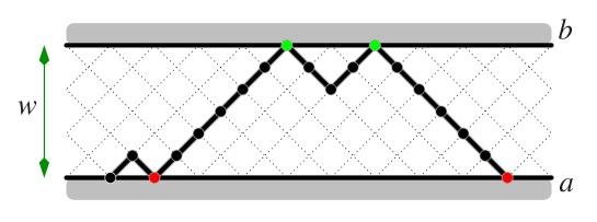
Figure 1: An example of a directed path which is a loop: both ends of the walk are fixed to be on the bottom wall.

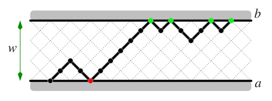
Figure 2: An example of a directed path which is a bridge: one end of the walk is fixed to be on the bottom wall ($y=0$) while the other end is fixed to be on the top wall ($y=w$).

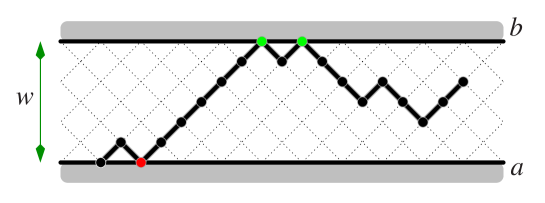
Figure 3: An example of a directed path which is a tail: one end of the walk is fixed to be on the bottom wall ($y=0$) while the other end is not constrained.

Let $\mathcal{L}_{w},\mathcal{B}_{w}$ and $\mathcal{T}_{w}$ be the sets of loops, bridges and tails, respectively, in the slit of width $w$. We define the generating functions of these paths as follows:

$$L_{w}(z,a,b) = \sum_{p\in\mathcal{L}_{w}}z^{n(p)}a^{u(p)}b^{v(p)};$$ (2.1)

$$B_{w}(z,a,b) = \sum_{p\in\mathcal{B}_{w}}z^{n(p)}a^{u(p)}b^{v(p)};$$ (2.2)

$$T_{w}(z,a,b) = \sum_{p\in\mathcal{T}_{w}}z^{n(p)}a^{u(p)}b^{v(p)},$$ (2.3)

where $n(p),u(p)$ and $v(p)$ are the number of edges in the path $p$, the number of vertices in the line $y=0$ (excluding the zeroth vertex) and the number of vertices in the line $y=w$, respectively.

Let $\mathcal{L}_{w}^{n},\mathcal{B}_{w}^{n}$ and $\mathcal{T}_{w}^{n}$ be the sets of loops, bridges and tails of fixed length $n$ in the slit of width $w$. The partition function of loops is defined as

$$Z_{n}^{loop}(w;a,b)=\sum_{p\in\mathcal{L}_{w}^{n}}a^{u(p)}b^{v(p)}$$ (2.4)

with the partition functions for bridges and tails defined analogously. Hence the generating functions are related to the partition functions in the standard way, eg for loops we have

$$L_{w}(z,a,b)=\sum_{n}z^{n}Z_{n}^{loop}(w;a,b).$$ (2.5)

We define the reduced free energy $\kappa^{loop}(w;a,b)$ for loops for fixed finite $w$ as

$$\kappa^{loop}(w;a,b)=\lim_{n\rightarrow\infty}n^{-1}\log Z_{n}^{loop}(w;a,b)$$ (2.6)

with the reduced free energies for bridges $\kappa^{bridge}(w;a,b)$ and tails $\kappa^{tail}(w;a,b)$ defined analogously.

Consider the singularities $z_{c}^{loop}(w;a,b)$, $z_{c}^{bridge}(w;a,b)$ and $z_{c}^{tail}(w;a,b)$ of the generating functions $L_{w}(z,a,b)$, $B_{w}(z,a,b)$ and $T_{w}(z,a,b)$, respectively, closest to the origin and on the positive real axis, known as the critical points. Given that the radii of convergence of the generating functions are finite, which we shall demonstrate, and since the partition functions are positive, the critical points exist and are equal in value to the radii of convergence. Hence the free energies exist and one can relate the critical points to the free energies for each $type$ of configuration, (that is loops, bridges and tails) as

$$\kappa^{type}(w;a,b)=-\log z_{c}^{type}(w;a,b).$$ (2.7)

Theorem 2.1.

Loops, bridges and tails have the same limiting free energy at every fixed finite $w$.

Proof.

We sketch the proof: Fix $w$ at some finite positive integer, and let $Z_{n}^{loop},Z_{n}^{bridge}$ and $Z_{n}^{tail}$ be the partition functions of loops, bridges and tails with $n$ edges in the strip of width $w$. By appending $w$ edges to loops and bridges we have the inequalities

$$bZ_{n}^{loop}\leq Z_{n+w}^{bridge}\qquad\mbox{ and }\qquad aZ_{n}^{bridge}\leq Z_{n+w}^{loop}.$$ (2.8)

Hence $abZ_{n}^{loop}\leq aZ_{n+w}^{bridge}\leq Z_{n+2w}^{loop}$. Taking logarithms, dividing by $n$ and taking the limit $n\to\infty$ shows that the limiting free energies are equal (since the limits exist).

Since every loop is a tail $Z_{n}^{loop}\leq Z_{n}^{tail}$, and by appending $w$ (if $n$ and $w$ have the same parity) or $w-1$ edges (if $n$ and $w$ have different parity) to tails we have

$$aZ_{n}^{tail}\leq Z_{n+w}^{loop}\qquad\mbox{ or }\qquad aZ_{n}^{tail}\leq Z_{n+w-1}^{loop},$$ (2.9)

depending on the parity of $n+w$. By a similar sandwiching argument the limiting free energies of loops and tails, and hence bridges, are all equal. ∎

Since the free energies are the same for the three models we define $\kappa(w;a,b)$ as

$$\kappa(w;a,b)\equiv\kappa^{loop}(w;a,b)=\kappa^{bridge}(w;a,b)=\kappa^{tail}(w;a,b)$$ (2.10)

with $z_{c}(w;a,b)$ being

$$z_{c}(w;a,b)\equiv z_{c}^{loop}(w;a,b)=z_{c}^{bridge}(w;a,b)=z_{c}^{tail}(w;a,b)$$ (2.11)

so that

$$\kappa(w;a,b)=-\log z_{c}(w;a,b).$$ (2.12)

3 The half-plane

For loops and tails we first consider the case in which $w\to\infty$, which reduces the problem to the adsorption of paths to a wall in the half-plane. We begin by noting that once $w>n$ for any finite length walk there can no longer be any visits to the top surface so

$$\mathcal{L}_{w+1}^{n}=\mathcal{L}_{w}^{n}\quad\mbox{ and }\quad\mathcal{T}_{w+1}^{n}=\mathcal{T}_{w}^{n}\mbox{ for all }w>n.$$ (3.1)

Hence we define the sets $\mathcal{L}_{hp}^{n}$ and $\mathcal{T}_{hp}^{n}$ as

$$\mathcal{L}_{hp}^{n}=\mathcal{L}_{n+1}^{n}\quad\mbox{ and }\quad\mathcal{T}_{hp}^{n}=\mathcal{T}_{n+1}^{n}.$$ (3.2)

The limit $w\to\infty$ can be therefore be taken explicitly. Also, as a consequence of the above, for all $w>n$ we have $v(p)=0$ for any $p\in\mathcal{L}_{w}^{n}$ and also for any $p\in\mathcal{T}_{w}^{n}$. Hence the partition function of loops in the half-plane can be defined as

$$Z_{n}^{loop,hp}(a)=\sum_{p\in\mathcal{L}_{hp}^{n}}a^{u(p)}$$ (3.3)

with the partition function of tails in the half-plane defined analogously. We define the generating function of loops in the half plane via the partition function as

$$L(z,a)=\sum_{n}z^{n}Z_{n}^{loop,hp}(a)$$ (3.4)

with the generating function of tails $T(z,a)$ in the half-plane defined analogously. Note that the above limit does not exist for bridges since for any fixed walk of length $n$ we have $w\leq n$. In an analogous way to the slit we define the reduced free energy in the half-plane for loops (and tails analogously) as

$$\kappa^{loop,hp}(w;a)=\lim_{n\rightarrow\infty}n^{-1}\log Z_{n}^{loop,hp}(w;a).$$ (3.5)

We note that in defining these free energies for the half-plane the thermodynamic limit $n\rightarrow\infty$ is taken after the limit $w\to\infty$: we shall return to this order of limits later.

While the half-plane solution is well known (Brak et al 1998, 2001 or Janse van Rensburg 2000) it is useful to summarise the main results for comparison with our new results for slits. One may factor both loops and tails in the half plane by considering the second last point at which a loop touches the line $y=0$ or the last point at which a tail touches the surface. This leads to the functional equations $L(z,a)=1+az^{2}L(z,a)L(z,1)$ and $T(z,a)=L(z,a)+zL(z,a)T(z,1)$ for the generating functions for loops and tails. These may be easily solved to give

$$L(z,a) = \frac{2}{2-a+a\sqrt{1-4z^{2}}}\quad\mbox{ and}$$ (3.6)

$$T(z,a) = \frac{4z}{(a-2-a\sqrt{1-4z^{2}})(1-2z-\sqrt{1-4z^{2}})}.$$ (3.7)

The generating functions are singular when the square root term is zero and when the denominator is zero. These conditions give the locations of the critical points, $z_{c}^{loop,hp}(a)$ and $z_{c}^{tail,hp}(a)$ and so also give the free energies. The values are equal for the two models and so we define $z_{c}^{hp}(a)\equiv z_{c}^{loop,hp}(a)=z_{c}^{tail,hp}(a)$, and similarly for the free energy we have

$$\kappa^{hp}(a)\equiv\kappa^{loop,hp}(a)=\kappa^{tail,hp}(a)=-\log z_{c}^{hp}(a)$$ (3.8)

with

$$\kappa^{hp}(a)=\left\{\begin{array}[]{cc}\log(2)&a\leq 2\\ \log\left(\frac{a}{\sqrt{a-1}}\right)&a>2.\end{array}\right.$$ (3.9)

The second derivative of $\kappa^{hp}(a)$ is discontinuous at $a=2$ and so there is a second-order phase transition at this point. The density of visits in the thermodynamic limit, defined as

$$\rho^{hp}(a)=\lim_{n\rightarrow\infty}\frac{\langle v\rangle}{n}=\frac{d\kappa^{hp}(a)}{d\log{a}}$$ (3.10)

is an order parameter for the transition and has corresponding exponent $\beta=1$.

4 Exact solution for the generating functions in finite width strips

The solution of the strip problem proceeds in an altogether different manner to the half-plane situation. This begins by using an argument that builds up configurations (uniquely) in a strip of width $w+1$ from configurations in a strip of width $w$. In this way a recurrence-functional equation is constructed rather than a simple functional equation. Consider configurations of any type — loops, bridges or tails — in a strip of width $w$ (see figure 4), and focus on the vertices touching the top wall: call these top vertices. These vertices contribute a factor $b$ to the Boltzmann weight of the configuration. Now consider a zig-zag path (see figure 4), which is defined as a path of any even length, or one of length zero, in a strip of width 1. The generating function of zig-zag paths is $1/(1-bz^{2})$. Replace each of the top vertices in the configuration by any zig-zag path. Since one could choose a single vertex as the zig-zag path all configurations that fit in a strip of width $w$ are reproduced. Also, the addition of any non-zero length path at any top vertex will result in a new configuration of width $w+1$ and no more. The inverse process is also well defined and so we can write recurrence-functional equations for each of the generating functions.

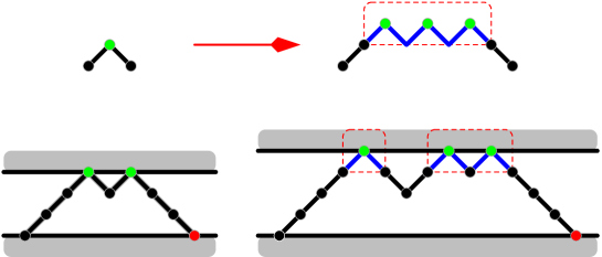
Figure 4: The construction of configurations in strip width $w+1$ from configurations in strip width $w$ is illustrated. Every vertex touching the upper wall in the strip of width $w$ can be replaced by a zig-zag path as shown.

The generating function $L_{w}(z,a,b)$ satisfies the following functional recurrence:

$$L_{1}(z,a,b) = \frac{1}{1-abz^{2}};$$ (4.1)

$$L_{w+1}(z,a,b) = L_{w}\left(z,a,\frac{1}{1-bz^{2}}\right).$$ (4.2)

The generating function of bridges, $B_{w}(z,a,b)$, satisfies a similar functional recurrence:

$$B_{1}(z,a,b) = \frac{bz}{1-abz^{2}};$$ (4.3)

$$B_{w+1}(z,a,b) = bz\;B_{w}\left(z,a,\frac{1}{1-bz^{2}}\right).$$ (4.4)

We note that the zeroth vertex of the path is weighted $1$ and that $L_{w}(z,a,b)$ counts the walk consisting of a single vertex. To compute the generating function of tails we introduce a new variable $c$ such that a tail whose last vertex is in the line $y=w$ is weighted by $c$. Using this variable we arrive at the following functional recurrence:

$$\tilde{T}_{1}(z,a,b,c) = \frac{(1+cz)}{1-abz^{2}};$$ (4.5)

$$\tilde{T}_{w}(z,a,b,c) = \tilde{T}_{w}\left(z,a,\frac{1}{1-bz^{2}},\frac{1+cz}{1-bz^{2}}\right).$$ (4.6)

The relevant tail generating function is then $T_{w}(z,a,b)=\tilde{T}_{w}(z,a,b,b)$.

Using these results it is easy to prove by induction that the generating functions for any finite $w$ must be ratios of polynomials in $z$. In fact using induction it is possible to prove that the generating functions $L_{w}(z,a,b)$, $B_{w}(z,a,b)$ and $\tilde{T}_{w}(z,a,b,c)$ have the following forms:

$$L_{w}(z,a,b) = \frac{P_{w}(z,0,b)}{P_{w}(z,a,b)},$$ (4.7)

$$B_{w}(z,a,b) = \frac{bz^{w}}{P_{w}(z,a,b)},$$ (4.8)

$$\tilde{T}_{w}(z,a,b,c) = \frac{Q_{w}(z,b,c)}{P_{w}(z,a,b)},$$ (4.9)

where the $P_{w}(z,a,b)$ and $Q_{w}(z,b,c)$ are polynomials. By simply iterating the recurrence-functional equations and using, for example the GFUN package of MAPLE^TM or by combinatorial means (Flajolet 1980 and Viennot 1985), one can find the recurrences $P_{w+1}=P_{w}-z^{2}P_{w-1}$ and $Q_{w+1}=(1+z)Q_{w}-z(1+z)Q_{w-1}+z^{3}Q_{w-2}$. The solution of these, using yet another generating variable $t$ over width $w$, gives

$$\qquad G_{p}(z,a,b,t)\equiv\sum_{w\geq 1}P_{w}(z,a,b)t^{w}=t\times\frac{(1-abz^{2})+(ab-a-b)z^{2}t}{1-t+z^{2}t^{2}}$$ (4.10)

and

$$\qquad G_{q}(z,a,b,c,t)\equiv\sum_{w\geq 1}Q_{w}(z,b,c)t^{w}=t\times\frac{(1+cz)-zt(c+bz)+cz^{3}t^{2}}{(1-zt)(1-t+z^{2}t^{2})}.$$ (4.11)

Alternately, one can find from substitution into the functional-recurrences (4.2) and (4.6) that

$$P_{w+1}(z,a,b)=(1-bz^{2})P_{w}(z,a,\frac{1}{1-bz^{2}})$$ (4.12)

and

$$Q_{w+1}(z,b,c)=(1-bz^{2})Q_{w}(z,\frac{1}{1-bz^{2}},\frac{1+cz}{1-bz^{2}}).$$ (4.13)

By multiplying both sides by $t^{w}$ and summing over $w$, one obtains functional equations for $G_{p}$ and $G_{q}$, which presumably can be solved directly. We note that $P_{w}$ and $Q_{w}$ are polynomials related to Chebyshev polynomials of the second kind (see for instance Abramowitz and Stegun 1972 or Szegö 1975) as can be seen by comparing generating functions. Other techniques such as transfer matrices (Brak et al 1999), constant term (Brak et al 1998) and heaps (Bousquet-Mélou and Rechnitzer 2002) would also undoubtedly work on these problems.

5 Location of the generating functions singularities

5.1 Transformation of the generating variable

We recall that the limiting free energy of a model is determined by the dominant singularities of its generating function. Since the generating functions of these three models are all rational with the same denominator, $P_{w}(z,a,b)$, it is the smallest real positive zero of this polynomial that determines the limiting free energy. Theorem 2.1 shows that this zero (since the only zero of the numerator for bridges is $0$ itself) is not cancelled by a zero of the numerator. Below we find the limiting free energy by studying the zeros of $P_{w}(z,a,b)$. Given $w$ we would like to find an expression for $z_{c}$ as a function of $a,b$.

Since the generating function $G_{p}(t)$ for the $P_{w}$ polynomials is a rational function of $t$ we can write it in partial fraction form with respect to $t$, and then expand each simple rational piece to find $P_{w}$ as a function of $w$. The decomposition of the right-hand side of (4.10) involves expressions containing surds which becomes quite messy. It is easier first to make a substitution that greatly simplifies the partial fraction decomposition and the subsequent analysis. This is chosen so as to simplify the denominator of $G_{p}(t)$. If we set

$$z=\frac{\sqrt{q}}{1+q}$$ (5.1)

the generating function of the polynomials then simplifies to

$$\qquad G_{p}(\sqrt{q}/(1+q),a,b,t) = ab-a-b+\frac{(1+q-aq)(1+q-bq)}{(1-q)(1+q-t)}$$ (5.2)

$$-\frac{(1+q-a)(1+q-b)}{(1-q)(1+q-tq)}$$

where there are simply linear factors in the denominator. The partial fraction expansion has been taken in (5.2). In our discussion of the singularities of $P_{w}$ we will start with this $q$-form. We can convert our results back later by making the inverse substitution

$$q=\frac{1-2z^{2}-\sqrt{1-4z^{2}}}{2z^{2}}.$$ (5.3)

The above partial fraction form implies that

$$\quad P_{w}(\sqrt{q}/(1+q),a,b)=\frac{(1+q-aq)(1+q-bq)}{(1-q)(1+q)^{w+1}}-\frac{(1+q-a)(1+q-b)q^{w}}{(1-q)(1+q)^{w+1}},$$ (5.4)

and when $a=0$ this simplifies to

$$\quad P_{w}(\sqrt{q}/(1+q),0,b)=\frac{(1+q-bq)}{(1-q)(1+q)^{w}}-\frac{(1+q-b)q^{w}}{(1-q)(1+q)^{w}}.$$ (5.5)

We also have

$$\qquad Q_{w}(\sqrt{q}/(1+q),a,b,c)= \frac{q^{\frac{1}{2}+w}\,\left(1-b+q\right)}{\left(1-{\sqrt{q}}\right)\,\left(1-q\right)\,{\left(1+q\right)}^{w}}$$ (5.6)

$$+\frac{1+q-b\,q}{\left(1-{\sqrt{q}}\right)\,\left(1-q\right)\,{\left(1+q\right)}^{w}}$$

$$-\frac{q^{\frac{w}{2}}\,\left(1-c-\left(b-2\,c\right)\,{\sqrt{q}}+\left(1-c\right)\,q\right)}{{\left(1-{\sqrt{q}}\right)}^{2}\,{\left(1+q\right)}^{w}}.$$

We can therefore find the generating functions for loops, bridges and tails. The generating function $L_{w}(\sqrt{q}/(1+q),a,b)$ can be written as

$$\qquad L_{w}=\frac{(1+q)\left[(1+q-bq)-(1+q-b)q^{w}\right]}{(1+q-aq)(1+q-bq)-(1+q-a)(1+q-b)q^{w}}.$$ (5.7)

Similarly $B_{w}$ and $T_{w}$ can be written as

$$\qquad B_{w}=\frac{bq^{w/2}(1-q)(1+q)}{(1+q-aq)(1+q-bq)-(1+q-a)(1+q-b)q^{w}}$$ (5.8)

and

$$\qquad T_{w}=\frac{\left(1+q\right)\,\left(q^{\frac{1+w}{2}}-1\right)\,\left(q^{\frac{w}{2}}\,\left(1-b+q\right)+\left(b-1\right)\,q-1\right)}{\left({\sqrt{q}-1}\right)\,\left(q^{w}\,\left(a-1-q\right)\,\left(b-1-q\right)-\left(\left(a-1\right)\,q-1\right)\,\left(\left(b-1\right)\,q-1\right)\right)}.$$ (5.9)

5.2 Limit $w\to\infty$ of the generating functions

In the limit that $w\to\infty$ we have, for $|q|<1$,

$$L_{w}(\sqrt{q}/(1+q),a,b) \to\frac{(1+q)}{1+q-aq},$$ (5.10)

$$T_{w}(\sqrt{q}/(1+q),a,b) \to\frac{(1+q)}{(1+\sqrt{q})(1+q-aq)}$$ (5.11)

and $$B_{w}(\sqrt{q}/(1+q),a,b) \to 0.$$ (5.12)

We note that substituting $z=z(q)$ back into the limits of $L_{w}$ and $T_{w}$ gives the generating functions of loops and tails adsorbing in a half-plane (equations 3.6 and 3.7) as required.

5.3 Singularities of the generating function of loops

Since each of the models has the same denominator polynomial this confirms that all three models have the same limiting free energy. To determine the free energy we examine the dominant singularity of the denominator polynomial.

The dominant singularity $q_{c}$ is the zero of the denominator of $L_{w}(q/(1+q),a,b)$ that has the minimal value of $|z|$, and hence is the solution of

$$q^{w}=\frac{(1+q-aq)(1+q-bq)}{(1+q-a)(1+q-b)}\$$ (5.13)

with this property.

Before discussing the cases in which we can find the singularity analytically, we first consider some examples where we locate the singularity numerically. To begin let us consider the symmetric case $a=b$ as this was also considered by DiMarzio and Rubin (1971). In figure 5 we plot $\kappa^{loop}(20;a,a)$ with the half-plane thermodynamic limit for comparison.

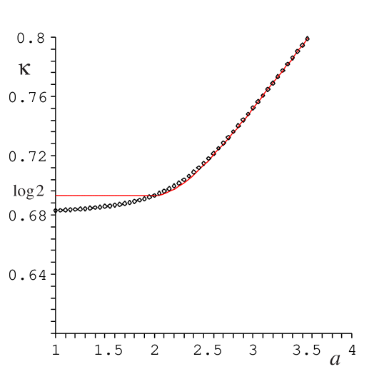
Figure 5: A plot of the free energy for width $w=20$ when $a=b$ is shown as the diamond markers. The solid curve is the half-plane solution.

For larger widths it is clear that the free energy converges to the half-plane curve as one might expect. Let us now consider weighting the vertices in the top wall such that they would strongly attract vertices of the polymer – one may expect this to hamper the convergence to the half-plane curve. Hence we consider $b=3$ and again for width $w=20$ plot the free energy $\kappa^{loop}(20;a,3)$: this can be found in figure 6.

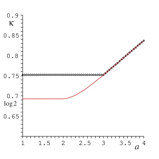
Figure 6: A plot of the free energy for width $w=20$ when $b=3$ is shown as the diamond markers. The solid curve is the half-plane solution.

It can now be seen that for $a<3$ the free energy is converging to something close to $0.75$ and not the half-plane curve which is $\log(2)$ for $a\leq 2$. Physically, we can understand that a long polymer in a slit with a highly attractive top wall will stick to that wall while the attraction of the bottom wall is lesser in magnitude. However, this points to the fact that this large width limit for infinitely long polymers does not demonstrate the same physics as the half-plane case.

6 Special parameter values of the generating function

The solutions of the equation (5.13) cannot be written in closed form for all values of $a$ and $b$. However, there are particular values for which this equation simplifies. When $a=1$ or $2$ and $b=1$ or $2$, and when

$$1-a=\frac{1}{1-b}\qquad\mbox{ equivalently }\qquad ab=a+b$$ (6.1)

the right-hand side of equation (5.13) simplifies. In these cases the locations of all the singularities of the generating functions can be expressed in closed form for all widths $w$. It is worth considering the generating function directly as some cancellations occur at these special points.

For the special values mentioned the generating functions $L_{w}$ and $B_{w}$ have particularly simple forms, while the forms for $T_{w}$ are slightly more complicated. We give the explicit form for $L_{w}$ at each of the points below:

• when $a=b=1$

  $$L_{w}=\frac{(1+q)(1-q^{w+1})}{1-q^{w+2}};$$ (6.2)

• when $a=2$ and $b=1$

  $$L_{w}=\frac{(1+q)(1-q^{w+1})}{(1-q)(1+q^{w+1})};$$ (6.3)

• when $a=1$ and $b=2$

  $$L_{w}=\frac{(1+q)(1+q^{w})}{1+q^{w+1}};$$ (6.4)

• when $a=b=2$

  $$L_{w}=\frac{(1+q)(1+q^{w})}{(1-q)(1-q^{w})};$$ (6.5)

• on the curve $ab=a+b$

  $$L_{w}=\frac{(1+q)((1+q-a)+(1+q-aq)q^{w})}{(1+q-a)(1+q-aq)(1-q^{w})}.$$ (6.6)

The singularities in $z$ of $L_{w}$, $B_{w}$ and $T_{w}$ may be found from the singularities in $q$ by the mapping (5.1). The singularities of $L_{w}$ in $q$ occur either for $|q|=1$ or for $q\in\mathbb{R}^{+}$. The transformation (5.1) maps $q\in\{|q|=1\}\cup\mathbb{R}^{+}$ to $z\in\mathbb{R}^{+}$. We note that if $q=e^{i\theta}$ then $1/z=2\cos(\theta/2)$. We concentrate on the dominant singularity $z_{c}$ for which $|z|$ is minimal.

Using the expressions for $L_{w}$ given above we find the zeros of the denominators (that do not cancel with a zero of the numerator) and choose the one that minimises $|z|$. This gives us $q_{c}$ and hence $z_{c}$. From these we find the free energy $\kappa$ at the special points listed above:

• when $a=b=1$ the zero is $q_{c}=\exp(2\pi i/(w+2))$ and hence

  $$\kappa(w;1,1)=\log\left(2\cos(\pi/(w+2))\right);$$ (6.7)

• when $a=1$, $b=2$ and when $a=2$, $b=1$ the zero is $q_{c}=\exp(\pi i/(w+1))$ and hence

  $$\kappa(w;2,1)=\kappa(w;1,2)=\log\left(2\cos(\pi/2(w+1))\right);$$ (6.8)

• when $a=b=2$ the zero is $q_{c}=1$ and hence

  $$\kappa(w;2,2)=\log(2);$$ (6.9)

• when $ab=a+b$ and $a\geq b$ the zero is $q_{c}=(a-1)^{-1}$ while when $ab=a+b$ and $b\geq a$ the zero $q_{c}=(b-1)^{-1}=(a-1)$. Hence for $a>1$

  $$\kappa(w;a,a/(a-1))=\log\left(\frac{a}{\sqrt{a-1}}\right).$$ (6.10)

In a similar way, one may write down expressions for the locations of all the singularities of the generating functions.

It is instructive to consider the free energy (see equation (6.10)) along the special curve given by $ab=a+b$. We first note that it is independent of the width of the slit. It is also clearly different at all values of $a<2$ to the half-plane free energy (which is $\log(2)$). This re-iterates that the large width limit of the slit problem is not necessarily described by the half-plane results.

In order to discuss the effective force between the walls for large $w$ we need to calculate the large $w$ asymptotics of the free energy. Since we have written down the closed form solution for all $w$ of $\kappa(w;a,b)$ at some special points it is advantageous to consider the large $w$ asymptotics of these first. As noticed above, on the curve $ab=a+b$ the $\kappa$ is independent of $w$ and so this includes the special point $(a,b)=(2,2)$. The large $w$ asymptotics for $\kappa$ for the remaining special points are calculated by expanding in inverse powers of $w$. They are

• when $a=b=1$

  $$\kappa(w,1,1)=\log(2)-\frac{\pi^{2}}{2w^{2}}+\frac{2\pi^{2}}{w^{3}}-\frac{72\pi^{2}+\pi^{4}}{12w^{4}}+O(w^{-5}),$$ (6.11)

• and when $(a,b)=(1,2)$ or $(2,1)$

  $$\quad\kappa(w,1,2)=\kappa(w,2,1)=\log(2)-\frac{\pi^{2}}{8w^{2}}+\frac{\pi^{2}}{4w^{3}}-\frac{72\pi^{2}+\pi^{4}}{192w^{4}}+O(w^{-5}).$$ (6.12)

7 Asymptotics for large widths at general parameter values

As we have noticed the large $w$ limit is dependent on the order of limits $w\rightarrow\infty$ and $n\rightarrow\infty$. As such we can now consider the large $w$ asymptotics of the free energy (which itself is first defined via an $n\rightarrow\infty$ limit). As mentioned above, we are interested in the forces between the walls for large $w$ which also involves large $w$ asymptotics. However, we are unable to find a closed form solution for $\kappa(w;a,b)$ for arbitrary $a,b$ and $w$. We can, however, find asymptotic expressions for $\kappa$ for arbitrary $a,b$ and large $w$ without the need for such an expression.

For general $a$ and $b$ the analysis depends on the region of parameter space and the plane naturally breaks up into various regions. These will become different phases when considering the limit $w\rightarrow\infty$. The analysis proceeds in a self-consistent manner perturbing around the solution obtained from the special points in descending powers of $w$.

For $a,b<2$ we can find the asymptotics of $q_{c}$ as a function of $w$,

$$q_{c}=\exp\left(2\pi i\Big{/}\left(w+\frac{2(a+b-ab)}{(2-a)(2-b)}\right)+O(w^{-4})\right),$$ (7.1)

which, mapping back to the $z$ variable, gives

$$\quad z_{c}=\frac{1}{2}+\frac{\pi^{2}}{4w^{2}}+\frac{\pi^{2}(ab-a-b)}{(2-a)(2-b)w^{3}}+\left(\frac{5\pi^{4}}{48}+\frac{3\pi^{2}(ab-a-b)^{2}}{(2-a)^{2}(2-b)^{2}}\right)\frac{1}{w^{4}}+O(w^{-5})$$ (7.2)

and so

$$\quad\kappa=\log(2)-\frac{\pi^{2}}{2w^{2}}-\frac{2\pi^{2}(ab-a-b)}{(2-a)(2-b)w^{3}}-\left(\frac{\pi^{4}}{12}+\frac{6(ab-a-b)^{2}}{(2-a)^{2}(2-b)^{2}}\right)\frac{1}{w^{4}}+O(w^{-5}).$$ (7.3)

For $b=2$ and $a<2$ we have

$$q_{c}=\exp\left(\pi i\Big{/}\left(w+\frac{a}{2-a}\right)+O(w^{-4})\right)$$ (7.4)

which gives

$$\qquad z_{c}=\frac{1}{2}+\frac{\pi^{2}}{16w^{2}}-\frac{\pi^{2}a}{8(2-a)w^{3}}+\left(\frac{5\pi^{4}}{768}+\frac{3\pi^{2}a^{2}}{16(2-a)^{2}}\right)\frac{1}{w^{4}}+O(w^{-5})$$ (7.5)

and so

$$\qquad\kappa=\log(2)-\frac{\pi^{2}}{8w^{2}}+\frac{\pi^{2}a}{4(2-a)w^{3}}-\left(\frac{\pi^{4}}{192}+\frac{3\pi^{2}a^{2}}{8(2-a)^{2}}\right)\frac{1}{w^{4}}+O(w^{-5}).$$ (7.6)

When $a=2$ and $b<2$ we obtain a similar expression where $b$ replaces $a$.

When $a$ or $b$ is greater than $2$ the asymptotic form changes. In particular the right-hand side of equation (5.13) is satisfied by either $q=1/(a-1)$ or $q=1/(b-1)$ and in the limit as $w\to\infty$ the left-hand side of the equation is zero. Hence we expand about the point $q=1/(a-1)$ and find that the next term in the expansion is exponential in $w$. More precisely, when $a>b$ and $a>2$ the asymptotic expansion of $q_{c}(w)$ as $w\to\infty$ is

$$\qquad q_{c}=\left(\frac{1}{a-1}\right)-\frac{a(a-2)(ab-a-b)}{(a-1)^{2}(a-b)}\left(\frac{1}{a-1}\right)^{w}+O\left(w\left(\frac{1}{a-1}\right)^{2w}\right).$$ (7.7)

Transforming this back to the $z$ variable gives

$$\qquad z_{c}=\frac{\sqrt{a-1}}{a}-\frac{(a-2)^{2}(ab-a-b)}{2a(a-b)\sqrt{a-1}}\left(\frac{1}{a-1}\right)^{w}+O\left(w\left(\frac{1}{a-1}\right)^{2w}\right)$$ (7.8)

and so the free energy is

$$\qquad\kappa=\log\left(\frac{a}{\sqrt{a-1}}\right)+\frac{(a-2)^{2}(ab-a-b)}{2(a-1)(a-b)}\left(\frac{1}{a-1}\right)^{w}+O\left(w\left(\frac{1}{a-1}\right)^{2w}\right).$$ (7.9)

For $b>a$ and $b>2$ one simply interchanges $a$ and $b$ in the above expressions to obtain the correct results.

Finally, when $a=b>2$ the asymptotic expansion of $q_{c}(w)$ is

$$q_{c}=\left(\frac{1}{a-1}\right)-\frac{a(a-2)}{(a-1)^{2}}\left(\frac{1}{a-1}\right)^{w/2}+O\left(w\left(\frac{1}{a-1}\right)^{w}\right)$$ (7.10)

and transforming this back to the $z$ variable gives

$$z_{c}=\frac{\sqrt{a-1}}{a}-\frac{(a-2)^{2}}{2a\sqrt{a-1}}\left(\frac{1}{a-1}\right)^{w/2}+O\left(w\left(\frac{1}{a-1}\right)^{w}\right)$$ (7.11)

and

$$\kappa=\log\left(\frac{a}{\sqrt{a-1}}\right)+\frac{(a-2)^{2}}{2(a-1)}\left(\frac{1}{a-1}\right)^{w/2}+O\left(w\left(\frac{1}{a-1}\right)^{w}\right).$$ (7.12)

8 The infinitely wide slit

We now come to consider the limit of large slits for infinite length polymers. Even though there isn’t a closed form solution for finite widths of the equation (5.13) we can simply use the large $w$ asymptotics above to deduce that

$$\qquad\kappa^{inf-slit}(a,b)\equiv\lim_{w\rightarrow\infty}\kappa(w;a,b)=\left\{\begin{array}[]{ll}\log(2)&\mbox{ if }a,b\leq 2\\ \log\left(\frac{a}{\sqrt{a-1}}\right)&\mbox{ if }a>2\mbox{ and }a>b\\ \log\left(\frac{b}{\sqrt{b-1}}\right)&\mbox{ otherwise.}\end{array}\right.$$ (8.1)

One immediately sees that the free energy depends on both $a$ and $b$ rather than only on $a$ which reflects the difference from the half-plane result (equation 3.9) noted earlier. In fact, the free energy is symmetric in $a$ and $b$ which reflects the observation that for infinitely long walks the end-points are irrelevant. For example, as in the case we considered earlier in figure 6 with $b>2$ the free energy for $a\leq b$ is $\log(\frac{b}{\sqrt{b-1}})$ (which is approximately $0.752$ for $b=3$) while it is $\log(\frac{a}{\sqrt{a-1}})$ for $a>b$. The half-plane phase diagram contains a desorbed phase for $a<2$ and an adsorbed phase for $a>2$. The transition between them is second order with a jump in the specific heat. Using (8.1) one can deduce for the infinite slit that there are 3 phases: one where the polymer is desorbed for $a,b<2$; a phase where the polymer is adsorbed onto the bottom wall for $a>2$ with $a>b$; and a phase where the polymer is adsorbed onto the top wall for $b>2$ with $b>a$. This is illustrated in figure 7.

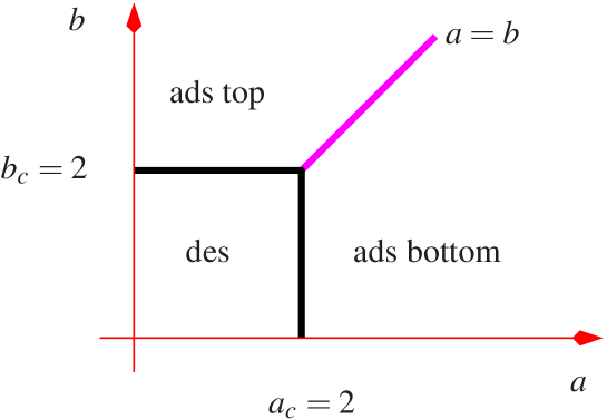
Figure 7: Phase diagram of the infinite strip. There are 3 phases: desorbed (des), adsorbed onto the bottom wall (ads bottom) and adsorbed onto the top (ads top).

The low temperature adsorbed phases are characterised by the order parameter of the thermodynamic density of visits to the bottom and top walls respectively. There are 3 phase transition lines. The first two are given by $b=2$ for $0\leq a\leq 2$ and $a=2$ for $0\leq b\leq 2$. These lines separate the desorbed phase from the adsorbed phases and are lines of second order transitions of the same nature as the one found in the half-plane model. There is also a first order transition for $a=b>2$ where the density of visits to each of the walls jumps discontinuously on crossing the boundary non-tangentially.

9 Forces between the walls.

Let us define the effective force between the walls induced by the polymer as

$$\mathcal{F}(w)=\frac{\partial\kappa(w)}{\partial w}=\frac{1}{z_{c}(w)}\frac{-\partial z_{c}(w)}{\partial w}.$$ (9.1)

Before examining the general case for large $w$ it is worth considering the general case for small $w$ numerically and at the special points for all $w$ where it can be found exactly. To begin, at the special points we can calculate the induced force exactly since we know the value of $\kappa(w)$ exactly. We note that since $\kappa(w)$ is monotonic at each of these points the induced force has one sign for all $w$. In particular,

• when $a=b=1$ then $1/z_{c}=2\cos(\pi/(w+2))$ and so

  $$\mathcal{F}=\frac{\pi}{(w+2)^{2}}\tan(\pi/(w+2))=\frac{\pi^{2}}{w^{3}}-\frac{6\pi^{2}}{w^{4}}+O(w^{-5})$$ (9.2)

  which is positive and hence repulsive.

• When $(a,b)=(2,1),(1,2)$ then $1/z_{c}=2\cos(\pi/2(w+1))$ and so

  $$\mathcal{F}=\frac{\pi}{2(w+1)^{2}}\tan(\pi/2(w+1))=\frac{\pi^{2}}{4w^{3}}-\frac{3\pi^{2}}{4w^{4}}+O(w^{-5})$$ (9.3)

  which is positive and hence repulsive.

• When $ab=a+b$ including $a=b=2$ then $1/z_{c}=\frac{\sqrt{a-1}}{a}=\frac{\sqrt{b-1}}{b}$ and so

  $$\mathcal{F}=0.$$ (9.4)

If one considers more general values of $a$ and $b$ numerically one observes that in each region of the phase plane $\kappa(w)$ is monotonic and hence the force takes on a unique sign at each value of $a$ and $b$. At general $(a,b)$ we are able to find the asymptotic force for large $w$ by using the large $w$ asymptotic expression for $\kappa(w;a,b)$ which we calculated above.

Using the asymptotic expressions for $\kappa$ found in section 7 in the $(a,b)$-plane we obtain the asymptotics for the force.

• For $a,b<2$

  $$\mathcal{F}=\frac{\pi^{2}}{w^{3}}+\frac{6\pi^{2}(ab-a-b)}{(2-a)(2-b)w^{4}}+O(w^{-5})$$ (9.5)

  which is positive and hence repulsive.

• For $b=2,a<2$

  $$\mathcal{F}=\frac{\pi^{2}}{4w^{3}}-\frac{3\pi^{2}a}{4(2-a)w^{4}}+O(w^{-5})$$ (9.6)

  which is positive and hence repulsive.

• For $a>b$ and $a>2$

  $$\qquad\mathcal{F}=-\frac{(a-2)^{2}(ab-a-b)\log(a-1)}{2(a-1)(a-b)}\left(\frac{1}{a-1}\right)^{w}+O\left(\left(\frac{1}{a-1}\right)^{2w}\right).$$ (9.7)

  For $b>a$ and $b>2$ one simply interchanges $a$ and $b$ in the above expressions to obtain the required result.

• At $b=a>2$

  $$\mathcal{F}=-\frac{(a-2)^{2}\log(a-1)}{4(a-1)}\left(\frac{1}{a-1}\right)^{w/2}+O\left(\left(\frac{1}{a-1}\right)^{w}\right).$$ (9.8)

  This is negative for all $a>2$ and so the induced force is attractive.

The regions of the plane which gave different asymptotic expressions for $\kappa$ and hence different phases for the infinite slit clearly also give different force behaviours. For the square $0\leq a,b\leq 2$ the force is repulsive and decays as a power law (ie  it is long-ranged) while outside this square the force decays exponentially and so is short-ranged. This change coincides with the phase boundary of the infinite slit phase diagram. However, the special curve $ab=a+b$ is a line of zero force across which the force, while short-ranged on either side (except at $(a,b)=(2,2)$), changes sign. Hence this curve separates regions where the force is attractive (to the right of the curve) and repulsive to the left of the curve. The line $a=b$ for $a>2$ is also special and, while the force is always short-ranged and attractive, the range of the force on the line is discontinuous and twice the size on this line than close by. All these features lead us to us a force diagram that encapsulates these features. This diagram is given in figure 8.

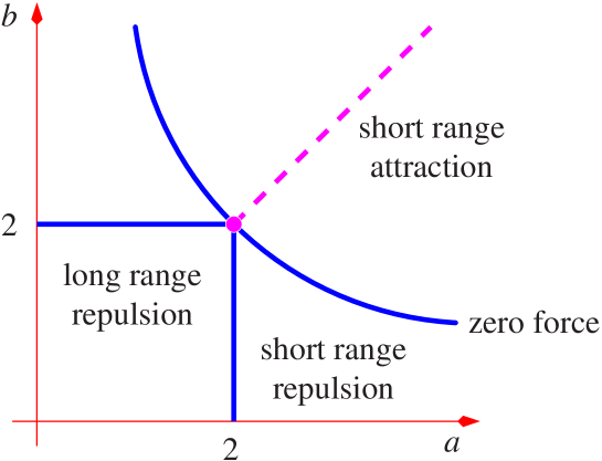
Figure 8: A diagram of the regions of different types of effective force between the walls of a slit. Short range behaviour refers to exponential decay of the force with slit width while long range refers to a power law decay. The zero force curve is the special curve given by $ab=a+b$. On the dashed line there is a singular change of behaviour of the force.

10 Discussion

We have solved and analysed in the limit of infinite length three types of polymer configuration, being loops, bridges and tails, in a two-dimensional slit geometry. The types of configurations considered are directed walks based on Dyck paths and the walks interact with both walls of the slit. We have found the exact generating functions at arbitrary width. We have calculated the free energy exactly at various points for arbitrary width, and, importantly, asymptotically (for large widths) for arbitrary $a$ and $b$. This has allowed us to map out the phase diagram for infinite slits: for finite width the free energy is an analytic function of the Boltzmann weights $a$ and $b$. This phase diagram is different to that obtained in the half-plane even though the generating functions for the half-plane are a formal limit of the finite width generating functions. This arises because the order of the infinite width and infinite polymer length limits (both of which are needed to see a phase transition) are not interchangeable.

From the large width asymptotics we have mapped regions of the plane where the free energy decreases or increases with increasing width and, also, whether this happens with an algebraic decay or exponential decay. Using this we have delineated regions where the induced force between the walls is short-ranged or long-ranged and whether it is attractive or repulsive. Three types of behaviour occur: long-ranged repulsive, short-ranged repulsive and short-ranged attractive. Applying such a model to colloidal dispersions implies that the regions where the force is long-ranged and repulsive support steric stabilisation while the regions where the force is short-ranged and attractive promote sensitized flocculation.

Given the curious interchange of limits phenomenon and from the point of view of the application of this theory to colloidal dispersions it would be interesting to investigate the finite polymer length cases both analytically and numerically with a view of searching for a scaling theory for the crossover from half-plane to slit type behaviour.

The model considered here is a directed walk in two dimensions. Although we expect the general features (such as the phase diagrams sketched in Figures 7 and 8) to be the same for self-avoiding walk models in both two and three dimensions, such models are beyond the reach of analytic treatments. It would be interesting to investigate the detailed behaviour of such models by Monte Carlo methods or by exact enumeration coupled with series analysis techniques.

References

Andre, D 1887 C. R. Acad. Sci. Paris 105 436–437

Abramowitz M and Stegun I A (Eds.). Orthogonal Polynomials. Ch. 22 in Handbook of Mathematical Functions with Formulas, Graphs, and Mathematical Tables, 9th printing. New York: Dover, 771–802, 1972.

Bertrand J 1887 C. R. Acad. Sci. Paris 105 369

Bousquet-Mélou M and Rechnitzer A 2002 Discrete Math. 258 235–274

Brak R, Essam J W and Owczarek A L 1998 J. Stat. Phys. 93 155–192

Brak R, Essam J W and Owczarek A L 1999 J. Phys. A. 32 2921–2929

Brak R and Essam J W 2001 J. Phys. A. 34 10763–10781

DiMarzio E A and Rubin R J 1971 J. Chem. Phys. 55 4318–4336

Deutsch E 1999 Discrete Math. 204 167–202

Flajolet P 1980 Discrete Math. 32 125–161

Hammersley J M and Whittington S G 1985 J. Phys. A: Math. Gen. 18 101–111

Janse van Rensburg E J, 2000 The Statistical Mechanics of Interacting Walks, Polygons, Animals and Vesicles, Oxford University Press, Oxford.

Middlemiss K M, Torrie G M and Whittington S G 1977 J. Chem. Phys. 66 3227–3232

Stanton D and White D, 1986 Constructive Combinatorics, Springer-Verlag.

Szegö G. Orthogonal Polynomials, 4th ed. Providence, RI: Amer. Math. Soc., 44–47 and 54–55, 1975.

Viennot G 1985 Lecture Notes in Mathematics 1171 139–157

Wall F T, Seitz W A, Chin J C and de Gennes P G 1978 Proc. Nat. Acad. Sci. 75 2069–2070

Wall F T, Seitz W A, Chin J C and Mandel F 1977 J. Chem. Phys. 67 434–438