Particle number renormalization in almost half filled Mott Hubbard superconductors
Bernhard Edegger1, Noboru Fukushima2,
Claudius Gros1, V.N. Muthukumar31 Institute for Theoretical Physics,
Universität Frankfurt, D-60438 Frankfurt, Germany
2 Department of Physics, University of the
Saarland, D-66041 Saarbrücken, Germany
3
Department of Physics, City College of the City University of New
York, New York, NY 10031
Abstract
The effects of the Gutzwiller projection on a BCS wave
function with varying particle number are considered. We show that a fugacity
factor has to be introduced in these wave functions when they are
Gutzwiller projected, and derive an expression for this factor
within the Gutzwiller approximation. We examine the effects of the
projection operator on BCS wave functions by calculating the
average number of particles before and after projection. We also
calculate particle number fluctuations in a projected BCS state.
Finally, we point out the differences between projecting BCS wave functions in the
canonical and grand canonical schemes, and discuss the relevance of our results for
variational Monte Carlo studies.
pacs:
74.20.-z, 74.20.Mn
I Introduction
Recently, Anderson has underscored the importance of fugacity in
wave functions that do not conserve particle number pwa_tunnel .
Following an earlier paper by Laughlin laughlin_02 ,
Anderson argued that a
fugacity factor should be included in variational wave
functions of the form,
(1)
Here, is a
(Gutzwiller) projection operator which excludes double occupancies
at sites (Ref. gutzwiller_63, ), and , a BCS wave function. Projected wave functions of
this form were originally proposed to describe the phase diagram
of doped Mott Hubbard insulators such as the high temperature
superconductors gros_88 ; RMFT ; atoz ; ys87 . Detailed variational
Monte Carlo (VMC) studies have been carried out recently using
projected -wave BCS states as variational wave functions for
the two dimensional Hubbard model, after a suitable canonical
transformation paramekanti ; gros87_almost .
Despite their simple form, projected wave functions exhibit nontrivial
properties because the projection operator acts on a quantum many body
state. The action of the projection operator (in reducing the allowed
states in the Hilbert space) concomitant with the correlations of
the quantum state being projected, leads to a variety of physical
phenomena variety . Other interesting effects include non-trivial
matrix-element renormalization near half-filling FEMG05
and the occurrence of superconductivity near an
(antiferromagnetic) Mott insulator afmi .
Approximate analytical calculations with wave functions
such as Eq. (1) can be done using a renormalization
scheme based on the Gutzwiller approximation.
Within this approximation, the effects
of projection on the state are
approximated by a classical statistical weight factor multiplying
the quantum result vollhardt_84 ; extensions .
Thus, for example,
(2)
where is any operator, and , the so called Gutzwiller
factor. For example, the Gutzwiller approximation for the
kinetic energy operator
and the superexchange interaction between sites
and , yields
the Gutzwiller factors,
(3)
where is the density of electrons.
In deriving these renormalization factors,
one considers
the number of terms that contribute to
and to
respectively.
The ratio of these two contributions is
the renormalization factor.
The renormalization factors are functions
of the local charge density. This is a well defined quantity
when one considers for example, a projected Fermi liquid state,
(4)
But suppose instead, we consider wave functions such as the BCS
state in Eq. (1), where the particle number fluctuates. In
this case, it is not clear what the local charge density in
Eq. (3) should be. It may be argued that the correct is set
by the average particle number . But then, projecting a
BCS state changes the average particle number; i.e., the
average number of electrons in does
not equal that in . Clearly, we need
a scheme to keep track of this effect.
Note that this problem can be avoided completely, as is done in
most variational Monte Carlo (VMC) studies. Here, the particle
number is fixed (one works in a canonical ensemble), and
Eq. (1) replaced by,
(5)
The operator fixes the particle number, and the issue of
projection changing the mean particle number does not arise
gros_88 . However, there are also other VMC studies with
wave functions that do not have fixed particle number
yokoyama_88 . Moreover, we are often interested in
carrying out analytical approximations in the spirit of
Eq. (2). Since such manipulations are easier done with BCS
wave functions (where the particle number is not fixed), it is
desirable to understand the effects of the projection operator on
this class of wave functions. In this paper, we present
analytical and numerical considerations of this problem. In doing
so, we clarify the notion of fugacity introduced by Anderson
pwa_tunnel . We also discuss the relevance
of this approach for the Gutzwiller approximation in the grand
canonical scheme and the corresponding VMC studies
yokoyama_88 .
II The fugacity factor
Consider the projected BCS wave function,
Eq. (1). It is clear that the projection operator changes the average number,
viz.,
The effect of the projection operator can be seen most clearly by
examining the particle number distribution in the unprojected and
projected Hilbert spaces. Towards this end, let us write the
average numbers, in the unprojected
(projected) Hilbert space
(6)
(7)
Here,
are the particle number distributions in the unprojected and
projected BCS wave functions respectively; is an operator
which projects onto terms with particle number . The particle number
distributions before and after projection may be related by
(8)
where
Eq. (8) constitutes the Gutzwiller approximation for the
projection operator with the corresponding renormalization
factor, ; is an irrelevant constant (the ratio of the
normalization of the unprojected and projected wave functions),
which does not depend on . Following Gutzwiller, we estimate
by combinatorial means, as being equal to
the ratio of the relative sizes of the projected and unprojected
Hilbert spaces. Then,
(9)
where is the number of lattice sites and
() is the number of up (down)-spins. Since in a
BCS wave function, , being
the total number of particles, the expression for can be
simplified to
(10)
Hence, if we were to impose the condition that the average
particle number before and after projection be identical, a factor
has to be included in Eq. (7). Then, from
Eq. (7) and Eq. (8), we obtain the particle number
after projection ,
(11)
which is the desired result.
Now, let us show how this
procedure can be implemented for the wave function
.
Since the BCS wave function is a linear superposition of states with
particle number , we consider the
effect of projection on two states whose particle numbers differ by .
Then, the ratio,
(12)
in the thermodynamic limit. Eq. 12 shows that the
projection operator acts unequally on the and particle
states; the renormalization of the weight of the particle
states , is times the
weight of the particle states, . This effect
can be rectified as in Eq. (11) by multiplying every
Cooper pair by a
factor in the BCS wave function. It produces the
desired result, viz., the projected and unprojected BCS
wave functions have the same average particle number.
Alternatively (following Anderson),
we can multiply every empty state by the factor and write,
(13)
Then again by construction, the fugacity factor in
Eq. (13) ensures that the projected wave function
and the unprojected wave
function have the same particle number.
The denominator in Eq. (13) is the new normalization factor.
The following points are in order: (a) the fugacity factor in
Eq. (12) depends on the variable particle number .
However, since the particle number of the BCS wave function is
sharply peaked within the range,
and
, we will assume that the
fugacity factor in the thermodynamic limit;
(b) in this limit, Eq. (12) reduces to , where
is the Gutzwiller factor defined in Eq. (3). Then,
Eq. (13) reduces to
(14)
which is the wave function proposed by Anderson pwa_tunnel ;
(c) the fugacity factor ensures that projection affects the
and particle states of the BCS wave function in the same
way. In principle, such a factor could depend on the -value,
but in this paper, we will treat it as a mere combinatorial device; (d) the
combinatorial argument fails at half filling when .
III Particle number renormalization
in projected BCS wave functions
In the previous section, we showed that the inclusion of the
fugacity factor is necessary for the average particle number in a
BCS wave function to be unchanged by projection. Alternatively,
one might ask what is the effect of the projection operator on a
BCS wave function; viz., if projection changes the mean
particle number of a BCS state, how are the particle numbers
before and after projection related? In this section, we will use
the fugacity factor to answer this question. In particular, we
will show how particle density after projection can be determined
self consistently by including the fugacity factor in the projected BCS
state (Eq. (14)). An alternate derivation of this result is
presented in Appendix A, where the effect of the
projection operator on particle number fluctuations is calculated.
Consider two BCS states defined by
(15)
(16)
where,
(17)
(18)
From Eq. (12), it is clear that the projection operator reduces the
ratio of the weights of and particle states in a BCS
wave function by a factor . Then, it follows that
(19)
when
(20)
The average particle number
of the state is
given by,
(21)
Since the particle numbers of and
are identical, we can use Eq. (18) in
Eq. (21) to obtain,
(22)
Note that is specified by the particle number after
projection, .
Now, since the number of particles in the state before projection is given by
Eq. (22) provides us with a way to calculate the number of
particles in the state
after projection, if
(i.e., and ) is specified before
projection. Eq. (22) can be solved self consistently for
. We solve Eq. (22) numerically on a square
lattice, using the standard BCS expressions for a -wave
superconductor, ():
(23)
(24)
where,
(25)
(26)
(27)
The only free parameters are the chemical potential and the variational
parameter .
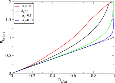
Figure 1:
(Color online)
Particle density before projection as a function
of the particle density after projection for
-wave states with different parameters .
The dashed line indicates the Fermi liquid
result .
By fixing the parameter , we determine the
particle numbers (before and after projection) for various
chemical potentials. The results for particle density () are shown in Fig. 1. The results clearly show that
the particle density before projection attains its maximal
value (), if (half-filling). This
result holds for any finite value of the variational parameter
. In the opposite limit, viz., low density of
electrons, converges to the value of as
expected. The size of the intermediate region depends on the
magnitude of the parameter , as illustrated by the results in
Fig. 1.
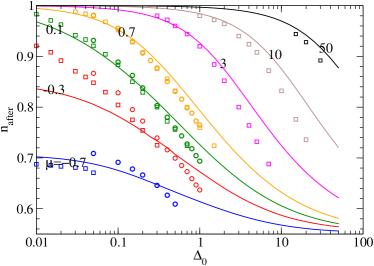
The accuracy of Eq. (22) can be checked by comparing our
results with those of Yokoyama and Shiba (YS), who performed VMC
studies of projected BCS wave functions with fluctuating particle
number (but without the fugacity factor) yokoyama_88 . They
determined the particle density of the projected -wave state
as a function of the chemical
potential and the variational parameter , within a grand
canonical scheme. The unprojected wave function is specified as usual, through
Eq. (23)-Eq. (27). Since YS do not include a
fugacity factor in their definition of the BCS wave function,
projection changes the particle number. So, we use Eq. (22)
to determine which we compare with their results for
particle number.
As seen in Fig. 2, our results
are in good qualitative agreement with YS. Discrepancies
are mostly due to finite corrections. YS use
and -lattices, while our analytic calculations
are for the thermodynamic limitinfiniteS .
The results show the singular effect of the projection near the
insulating phase (half filling). The chemical potential goes to
infinity in this limit.
Figure 2: (Color online)
The particle density after projection as a
function of parameter for a -wave BCS
state at various chemical potentials . The figure shows a
comparison between results from Eq. (22)(solid lines) and the
VMC results of Yokoyama and Shiba yokoyama_88 (for
- (circles) and -lattices (squares)).
Numbers in the figure denote the chemical potentials of the
corresponding curves and data points.
In Appendix A, we present an alternate derivation of Eq. (22)
by a saddle point approximation
without using a fugacity-corrected wave function. This approach
also allows for the calculation of particle number fluctuations .
IV Gutzwiller approximation in the canonical and grand canonical schemes
In this section, we discuss the differences between the Gutzwiller
approximation in the canonical and grand canonical schemes. The
validity of our statements can be checked by a comparison to nearly
exact VMC yokoyama_88 ; gros_88 ; paramekanti ; yokoyama_96 .
Let us first consider the canonical case. Here, we are
interested in the expectation value of an operator
calculated with a particle number conserving projected wave function
. The corresponding
Gutzwiller approximation can be understood as follows:
(28)
where is the projector on the terms with particle number
. The Gutzwiller factor , corresponds to the
operator . The first row represents a quantity which can be
calculated exactly by fixed particle number VMC
gros_88 ; paramekanti . Since the particle number is fixed,
the Gutzwiller approximation can be invoked, leading to the second
row. The equality to the third row is guaranteed only if is
equal to the average particle number of (). Here, we perform a transformation
from a canonical to a grand canonical ensemble, which is
valid in the thermodynamic limit.
In the grand canonical scheme, where we calculate the
expectation value of with a particle number non-conserving
wave function, this scheme must be modified as follows:
(29)
where is the projected
-wave state corrected for fugacity, i.e., a fugacity
factor is included simultaneously with the projection (see
Sec. II). This correction is essential to guarantee
the validity of the Gutzwiller approximation; without it,
the lhs and rhs of Eq. (29) would correspond to
states with different particle numbers.
Eq. (29) and Eq. (30) constitute the main results of this section.
Eq. (29) shows that when the Gutzwiller approximation is used for a wave function
which does not have a fixed particle number, a fugacity factor must be included along with the projection. Eq. (30) shows that to obtain
identical results, one has to use
different wave functions
in the grand canonical (rhs) and
canonical (lhs) schemes. The wave function
is a -wave state corrected
by the fugacity factor, whereas is
a pure -wave state. Our arguments leading up to Eq. (29) and Eq. (30) can be verified by a comparison with VMC studies. We now proceed to do so.
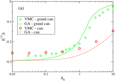
The expectation values in the canonical and grand canonical schemes
can be calculated (nearly exactly) by VMC studies. In
Fig. 3, we show VMC results from Gros gros_88
(fixed particle number VMC, canonical) and from YS
yokoyama_88 (grand canonical VMC). The discrepancy between
the two sets of results can be explained readily by Eq. (30).
In the case of , there is only small room
for particle number fluctuations even in the particle
non-conserving wavefunction. Then, canonical and grand canonical
schemes should give identical results. The VMC calculations in
Fig. 3 do not exactly show thit behavior since the
grand-canonical scheme becomes inaccurate in this limit
yokoyama_88 . YS consider a pure -wave state,
i.e., the fugacity factor is not included in their
calculations. In their paper, YS argued that the discrepancies
between the two results can be removed by introducing an
additional variational parameter , so that is replaced by (Eq. 4.1 in
Ref. yokoyama_88, ). We opine that the parameter
is directly related to our fugacity factor,
i.e., in the wave function
. This conclusion is supported
by the comparison of VMC data to the corresponding Gutzwiller
approximation (see below).
The validity of the approximation in the canonical case
(Eq. (28)) is well accepted. It is used for instance, in the
renormalized mean field theory (RMFT) of Zhang et al.,
where all physical quantities are calculated using unprojected
wave functions and the corresponding Gutzwiller renormalization
factors RMFT . A comparison with VMC studies with fixed
particle number shows good agreement RMFT (also
illustrated in Fig. 3).
To compare the grand canonical VMC of YS with the Gutzwiller
approximation, we need to modify Eq. (29). This is necessary because YS do not include the fugacity factor in their considerations, as pointed out earlier.
We modify Eq. (30) by the following procedure:
(i) we start with a
-wave BCS state for specified
values of ;
(ii) we use Eq. (22) to
determine the chemical potential . This fixes the particle
density of ;
(iii) we remove the fugacity factor to get via Eq. (16). The fugacity
factor is determined for . and correspond to
the same particle density .
(iv) The expectation values of the wave function can now be approximated by and Gutzwiller factors, viz.,
(31)
This Gutzwiller approximation (GA) generalizes Eq. 2
for wave functions that do not conserve particle number.
In Appendix B, we discuss this approximation for the different terms in the model.
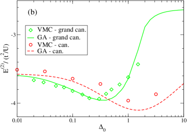
In Fig. 4, we compare the GA of the kinetic energy
, and the expectation value , of the remaining
terms in the model (,
, and the 3-site term) to those
from the grand canonical VMC. A good agreement between the VMC and
Gutzwiller results is seen, which confirms the validity of our
grand canonical Gutzwiller approximation (Eq. (29)).
Figure 3:
(Color online)
(a) The kinetic energy
and (b) the energy of the remaining terms per site of
the model as a function of the variational
parameter for the -wave state
at a filling . Fixed particle (can.) VMC
datagros_88 (circles, 82 sites) and grand canonical
VMCyokoyama_88 (squares, sites) are compared.
The dashed/solid lines represent the corresponding Gutzwiller
approximations (GA). For a detailed description, we refer to the
text and Appendix B.
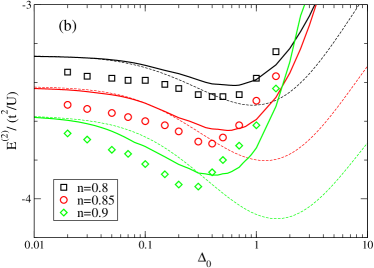
Figure 4:
(Color online)
(a) The kinetic energy and (b) the energy of the remaining
terms per site of the model, as a function of the variational
parameter for the -wave state at various densities. The data
points (diamond, circle, square) are taken from the grand
canonical VMC study of Yokoyama and Shiba yokoyama_88 . The
solid/dashed lines represent
the corresponding Gutzwiller approximations for a
grand canonical/fixed-particle VMC study. For a detailed
description, we refer to the text and Appendix
B.
In Fig. 3 and Fig. 4, we also show
Gutzwiller approximations for the fixed particle number VMC
gros_88 . Clearly, canonical and grand canonical approaches yield different energies
(as do the corresponding VMC studies ). We emphasize this is
because of the projection operator , which changes the particle number
in a grand canonical scheme. For these two methods to yield the
same results, a fugacity corrected wave function must be used when
working in a grand canonical ensemble. Hence, all previous
speculations about the coincidence of these two VMC schemes in the
thermodynamic limit
have to be reformulated carefully.
V Summary
In this paper, we considered the effects of Gutzwiller projection on a state which
does not have fixed particle number. We showed that it is necessary to include
a fugacity factor when invoking the Gutzwiller approximation for such states.
The effects of projecting a number non-conserving BCS state were studied by
examining
the relation between particle number before and
after projection. We obtained an analytical expression,
Eq. (22), and compared to variational
Monte Carlo data (Fig. 2). We discussed the
discrepancies in the VMC results for projected BCS wave functions obtained in the
canonical and grand canonical schemes, and presented a resolution.
In conclusion,
we have clarified several subtle properties of the Gutzwiller
projection operator acting on a BCS state, and hope that these results lead to a better
understanding of the Gutzwiller approximation in the grand canonical scheme.
We thank P. W. Anderson, N. P. Ong, and H. Yokoyama for several
discussions. N. F. was supported by the Deutsche
Forschungsgemeinschaft. V. N. M. acknowledges partial financial
support from The City University of New York, PSC-CUNY Research
Award Program.
Appendix A Saddle point approximation
to mean particle number and number fluctuations
in projected BCS wave functions
In Sec. III, we used the fugacity factor to derive Eq. (22).
Here, we present an alternative approach by a
saddle point approximation to discuss the effects of
projection on the mean particle number of a BCS state. This
approach also describes the particle number fluctuations after
projection.
The particle number distribution for an unprojected BCS
wave function can be written as
(32)
where is the number of electron pairs. This
relation can be checked by expanding the product in the wave
function,
and considering contribution to from each term. In Sec. III, we showed that the particle
number distribution of a projected wave function is
related to the unprojected distribution by
(33)
where,
Particle number and number fluctuations of the projected wave function
can be derived from Eq. (33) and Eq. (32), upon invoking a saddle
point approximation.
We define a generating function ,
(34)
We invert Eq. (34) using a contour integral
on the complex -plane along a circle around :
(35)
Note that, in the integrand, only gives a finite value.
The others powers of vanishes. Multiplying by
gives
for the average particle density of a projected BCS wave function.
Without the factor this calculation would give the well known result
for an unprojected BCS wave function,
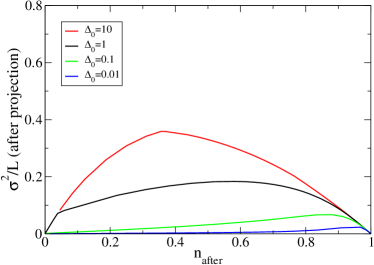
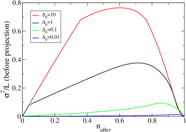
Figure 5: (Color online)
The fluctuation / after/before projection
for different values of the variational parameter
, as a function of the particle
density after projection .
To calculate the particle number fluctuations of the projected
wave function, we need to expand up to second order
in and around the saddle point. Then,
integration over in Eq. (37) approximates the
particle number distribution by a gaussian distribution,
yielding an expression for number fluctuations. With
the second order expansion can be written as
(44)
For this level of the saddle point approximation for ,
the contour around for the integral in Eq. (37) must be taken so that
. Since
and contribution only
near the saddle point is relevant, the path is taken from
to . By variable
transformation , one can
perform a gaussian integral of . Then, we obtain a
a gaussian distribution for ,
(45)
The variance of (average particle number of a projected
BCS wave function) can now be read off from Eq. (45). We
get,
(46)
where we used Eq. (41) in the second term. For
we must insert . For completeness, we mention that for the
unprojected wave function, i.e. not included, this
approach yields the known result
(47)
The fluctuations are illustrated in
Fig. 5 as a function of the particle density after
projection for unprojected () and projected () BCS -wave functions. As expected, the fluctuations vanish at half filling, since projection freezes the charge degrees of freedom entirely.
Appendix B Gutzwiller approximation for the Hamiltonian
We summarize the Gutzwiller approximation for the so-called 3-site
terms in the model, that are included in the VMC study of
Yokoyama and Shiba yokoyama_88 .
The model can be derived from a large expansion of the
Hubbard model. The Hamiltonian is valid in the reduced
Hilbert space of no double occupied states, and is given by
(48)
where
(49)
and
(50)
Here, , are the spin operators on site
, and with
. are pairs of n.n sites and denotes a n.n. site
of .
We are interested in the energies and
calculated in Ref. yokoyama_88, :
(51)
We invoke the Gutzwiller approximation. The renormalization
factors, for kinetic energy (Eq. (49)) and for spin
exchange (first term in Eq. (50)), are given in Eq. (3). The
second term of Eq. (50), , is not renormalized. The
approximation for the 3-site terms (3rd and 4th term of
Eq. (50)) is done as follows ():
(52)
(53)
The renormalization factor is derived by considering the
number of terms that contribute to the projected and the
unprojected side respectively. The projected side (lhs) contributes only
if (i) site is unoccupied, i.e., probability
, (ii) site is singly occupied by a
-electron, i.e., probability ,
and (iii) site is singly occupied by an
-electron, i.e., probability . On
the other hand, the unprojected side (rhs) in Eq. (52)/Eq. (53)
contributes only if (i) site is not occupied by an
-electron/-electron, i.e.,
probability / , (ii) site
is singly occupied by a -electron, i.e.,
probability , and (iii) site
must have an -electron, i.e.,
probability . These probabilities yield the Gutzwiller
factor (ratio of contributions from projected and unprojected
states),
(54)
where we assumed .
We can now write down the renormalized Hamiltonian
,
(55)
where,
(56)
(57)
By using and , Eq. (51)
( and ) can be calculated using unprojected
wave functions,
(58)
Evaluating Eq. (58) by Wick’s decomposition for a
-wave BCS state,
(59)
where we defined ()
The last three rows in Eq. (59) correspond to the 3-site
terms of the model and are renormalized by the Gutzwiller
factor . Here, it’s important to note that
the order parameter is related, but not identical,
to the previous introduced variational parameter .
References
(1)
P. W. Anderson (private communication) and
P. W. Anderson and N. P. Ong, cond-mat/0405518.
(2)
R. B. Laughlin, cond-mat/0209269.
(3) M. C. Gutzwiller, Phys. Rev. Lett.
10, 159 (1963).
(4) Claudius Gros, Phys. Rev. B 38, 931 (1988).
(5) F. C. Zhang, C. Gros, T. M. Rice and H. Shiba,
Supercond. Sci. Tech. 1 36 (1988); also available as cond-mat/0311604.
(6)
P. W. Anderson, P. A. Lee, M. Randeria, T. M. Rice, N. Trivedi and
F. C. Zhang, J. Phys. Cond. Mat. 16 R755 (2004).
(7) H. Yokoyama, and H. Shiba,
J. Phys. Soc. Jpn. 56, 1490 (1987).
(8) A. Paramekanti, M. Randeria and N. Trivedi,
Phys. Rev. Lett. 87 217002 (2001);
Phys. Rev. B 69 144509 (2004);
Phys. Rev. B 70, 054504 (2004).
(9) C. Gros, R. Joynt, T.M. Rice,
Phys. Rev. B 36, 381 (1987).
(10)
Jörg Bünemann, Florian Gebhard, Torsten Ohm, Stefan Weiser, and
Werner Weber, cond-mat/0503332; D. Jaksch, C. Bruder, J. I. Cirac, C. W. Gardiner, and
P. Zoller, Phys. Rev. Lett. 81 3108 (1998);
M. Bak and R. Micnas, J. Phys.: Cond. Matt. 10, 9029 (1998);
B. R. Bulka and S. Robaszkiewicz,
Phys. Rev. B 54, 13138 (1996).
Jian Ping Liu, Phys. Rev. B 49, 5687 (1994);
Daniel S. Rokhsar and B. G. Kotliar,
Phys. Rev. B 44, 10328 (1991);
K. Seiler, C. Gros, T. M. Rice, K. Ueda, D. Vollhardt,
J. Low. Temp. Phys. 64, 195 (1986).
(11) N. Fukushima, B. Edegger, V.N. Muthukumar, C. Gros,
cond-mat/0503143.
(12) T. K. Lee, Chang-Ming Ho and Naoto Nagaosa, Phys. Rev. Lett. 90,
067001 (2003); Hisatoshi Yokoyama, Yukio Tanaka, Masao Ogata, and Hiroki Tsuchiura, J. Phys. Soc. Jpn 73, 1119 (2004); J.Y. Gan, Y. Chen, Z B. Su, F.C. Zhang,
Phys. Rev. Lett. 94, 067005 (2005).
(13) D. Vollhardt, Rev. Mod. Phys. 56, 99 (1984).
(14) Several extensions to the Gutzwiller approximation have been proposed in the literature. See, for instance, M. Ogata and A. Himeda, J.Phys. Soc. Jpn. 72, 374 (2003); G. Seibold, and J. Lorenzana, Phys. Rev. Lett. 86, 2605 (2001);
M. Lavagna, Phys. Rev. B 41, 142 (1990).
(15) H. Yokoyama, and H. Shiba,
J. Phys. Soc. Jpn. 57, 2482 (1988); H. Yokoyama (private communication).
(16) By infinite system size, we mean that
the sum over all in Eq. (22) is transformed
into an integral. In the VMC studies the sum over is
considered on a finite system, i.e., a finite number of
-values. Generally the resulting finite size effects are
small yokoyama_96 , and a direct comparison to an infinite
system is reasonable.
(17) H. Yokoyama, and M. Ogata,
J. Phys. Soc. Jpn. 65, 3615 (1996).