Wave trains, self-oscillations and synchronization in discrete media

Abstract

We study wave propagation in networks of coupled cells which can behave as excitable or self-oscillatory media. For excitable media, an asymptotic construction of wave trains is presented. This construction predicts their shape and speed, as well as the critical coupling and the critical separation of time scales for propagation failure. It describes stable wave train generation by repeated firing at a boundary. In self-oscillatory media, wave trains persist but synchronization phenomena arise. An equation describing the evolution of the oscillator phases is derived.

1 Introduction

Understanding wave propagation and self-oscillations in discrete media is important to predict the behavior of many biological and physical systems composed of smaller interacting units, such as cells, nodes, atoms, wells… Examples abound: propagation of impulses through myelinated axons [25] or cardiac tissue [2], voltage oscillations in muscle fibers [22], charge transport in semiconductor superlattices [4], crystal growth and interface motion in crystalline materials [6], etc.

In this paper, we consider an infinite chain of diffusively coupled cells described by a fast variable $v_{n}$ and a slow variable $w_{n}$:

$${dv_{n}\over dt}=D(v_{n+1}-2v_{n}+v_{n-1})+f(v_{n},w_{n}),$$ (1)

$${dw_{n}\over dt}=\lambda g(v_{n},w_{n}).$$ (2)

Typically, $v_{n}(t)$ represents the ratio of the membrane potential to some reference equilibrium potential and $w_{n}(t)$ the fraction of open channels for some type of ions at the $n$-th site. The parameter $D>0$ measures the strength of the coupling and $\lambda>0$ represents the ratio of the time scales for $v_{n}$ and $w_{n}$. $\lambda$ must be small enough for the two variables to evolve in different time scales. We assume that the nullclines $g(v,w)=0=f(v,w)$ intersect at one point, the equilibrium of the system. For $w$ fixed, the source $f(v,w)$ is bistable. System (1)-(2) displays excitable or self-oscillatory behavior depending on whether the equilibrium state is stable or unstable.

In the excitable case, periodic disturbances in the medium lead to propagation of signals in the form of wave trains. To obtain analytic information on those waves, it is quite tempting to replace the discrete system (1)-(2) by its continuum limit $D\rightarrow\infty$:

$${\partial v\over\partial t}={\partial^{2}v\over\partial x^{2}}+f(v,w),\quad{\partial w\over\partial t}=\lambda g(v,w).$$ (3)

There is a good mathematical reason not to do that: propagation failure. The discrete system has a threshold coupling for wave propagation whereas the continuous model allows wave propagation at all coupling strengths. Constructing wave train solutions of discrete systems is not easy. An asymptotic understanding of these solutions and their numerical construction have to go hand in hand. In an infinite chain, most initial conditions will either fail to propagate or evolve into a solitary pulse. Only very particular initial conditions evolve into a wave train, as we will show later in this paper after explaining the asymptotic construction thereof. Simpler pulse solutions were constructed asymptotically in [9] for the discrete FitzHugh-Nagumo model. For continuous models, asymptotic descriptions of pulse waves are given in [16]. Unlike continuous model equations, travelling waves in discrete media do not solve a system of ordinary differential equations. Instead, a more complex system of differential-difference equations needs to be analyzed. Rigorous results are only available for particular sources and traveling pulses. Tonnelier [26] found explicit expressions of pulses for piecewise linear sources. Existence of discrete pulses has been proved for a restricted class of nonlinear sources [11]. Conditions for propagation failure were discussed in [1, 5, 9].

In this paper, we give an asymptotic construction of wave trains in discrete excitable systems. Solitary pulses are a particular case of a wave train with infinite spatial period and maximum speed. We study the dynamic equations (1)-(2) for general smooth nonlinear source terms. Experimental values of $D$ (for instance in nerve models) are typically small. Thus, we focus in the highly discrete case: $D\ll 1$. We find a one-parameter family of stable wave trains and we predict their speed, period and shape, as well as the critical coupling for propagation failure. Near the critical coupling, the profiles develop steps as shown by Figure 6(b) and Figure 8. Propagation is ‘saltatory’: it proceeds by a sequence of successive jumps. The mechanism for propagation failure as the coupling decreases is reminiscent of the depinning transitions for wave fronts described in [8]. Propagation also fails when the parameter $\lambda$ characterizing the ratio of time scales is no longer small. Our asymptotic construction yields sharp upper an lower bounds on the critical value of $\lambda$ below which propagation fails, $\lambda_{c}(D)$, as a function of the coupling $D$. For $D$ small, we also obtain an asymptotic prediction which describes accurately numerical measurements. Technically, we have greatly improved the rough bounds contained in [11], derived under very restrictive assumptions on the nonlinearities. Bounds on the critical separation of scales are unknown in the continuum case.

When the medium is self-oscillatory, the mechanism leading to periodic wave train generation is completely different. Spatially uniform profiles corresponding to stable limit cycles of the system:

$${dv\over dt}=f(v,w),\;{dw\over dt}={\lambda}g(v,w),$$ (4)

play a key role and introduce new features such as synchronization. For small couplings, we derive an equation for the time evolution of oscillator phases.

The paper is organized as follows. In section 2 we give an asymptotic description of periodic wave trains for excitable systems. Section 3 discusses their numerical stability and selection via initial and boundary conditions. We use the FitzHugh-Nagumo (FHN) and the more complicated Morris-Lecar (ML) dynamics as examples in our numerical calculations. Section 4 analyzes the impact of discreteness on propagation failure. We predict the critical coupling and the critical separation of time scales for propagation failure as a function of the coupling. Section 5 is devoted to self-oscillatory behavior and synchronization. Section 6 contains our conclusions.

2 Wave trains and pulses in excitable media

Figure 1 depicts the nullclines for system (1)-(2) and the sources we have used in the numerical tests. We assume that the source $f(v,w)$ is a cubic function of $v$ with three zeros $z_{1}(w)<z_{2}(w)<z_{3}(w)$, the first and the third of which are stable for the reduced equation (1) with $w_{n}=w$. The nullclines must intersect in the first or third branch of the cubic to guarantee that (1)-(2) describe an excitable system. Intersections of the nullclines in the middle branch of the cubic correspond to unstable stationary states and give rise to self-oscillatory dynamics. To fix ideas, we assume in this section that the nullclines intersect at a point $(v^{0},w^{0})$ located in the first branch of the cubic.

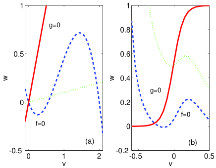
Figure 1: (a) FHN with $a=0.3$ and $b=0.5$ (solid), $b=10$ (dotted); (b) ML with $I=0.0625$ (dashed), $0.375$ (dotted).

Experimental values of $D$ (for instance in nerve models) are typically small. Thus, we focus in highly discrete problems with $D\ll 1$. As shown in Figure 2, a wave train resembles a sequence of pulses. After a short transient the system relaxes to a traveling wave: $v_{n}(t)=V(n-ct)$, $w_{n}(t)=W(n-ct)$, in which $V$ and $W$ are periodic functions with the same period $L$. This defines the wave profiles $V(z)=v_{n}({n-z\over c})$ and $W(z)=w_{n}({n-z\over c})$, $z=n-ct$. Neighboring points describe the same trajectory with a time delay ${1\over c}$: $v_{n+1}(t)=v_{n}(t-{1\over c}),$ $w_{n+1}(t)=w_{n}(t-{1\over c})$.

The profiles and speeds solve an eigenvalue problem for a system of differential-difference equations:

$$\begin{array}[]{l}-cV_{z}(z)\!=\!D\!(V(z\!+\!1)\!-\!2V(z)\!+\!V(z\!-\!1))\!+\!f(V(z),W(z)),\\ -cW_{z}(z)\!=\!\lambda g(V(z),W(z)),\end{array}$$ (7)

with $V(z+L)=V(z)$, $W(z+L)=W(z)$. Equations (7) are hard to solve except in very particular situations, such as piecewise linear $f$ and linear $g$ [26]. Is there an alternative way to extract practical information on the waves? We show below how to use asymptotic methods to predict the ranges of the parameters for which we expect stable wave trains to be formed, the shape of their profiles, their spatial period $L$ and speed $c$.

2.1 The reduced bistable equation

As Figure 2 shows, a wave train for $v_{n}$ is a sequence of sharp interfaces separated by smooth transitions. At the interfaces, the recovery $w_{n}$ is almost constant. Thus, the first step in our asymptotic construction is the study of wave front propagation in the bistable equation:

$${dv_{n}\over dt}=D(v_{n+1}-2v_{n}+v_{n-1})+f(v_{n},w).$$ (8)

Choosing $w$ in a neighborhood $(w_{-},w_{+})$ of the equilibrium value $w^{0}$, the source $f(v,w)$ has three zeros $z_{1}(w)<z_{2}(w)<z_{3}(w)$, the first and the third of which are stable. The parameter $w$ controls the degree of asymmetry of the source, as shown in Figure 3(b). In particular, it changes the ratio of the area $A_{12}$ above $f$ between $z_{1}$ and $z_{2}$ and the area $A_{23}$ below $f$ between $z_{2}$ and $z_{3}$. When the cubic source $f(v,w)$ is asymmetric enough, depending on $D$, wave fronts $v_{n}=V(n-ct)$ joining the two stable zeros $z_{1}(w)$ and $z_{3}(w)$ propagate [7, 8, 12, 21, 27]. Generically, there are two threshold values $w_{c-}(D)$,$w_{c+}(D)$ such that:

• If $w\in(w_{-},w_{c-}(D))$, wave fronts decreasing from $z_{3}(w)$ to $z_{1}(w)$ (resp. increasing from $z_{1}(w)$ to $z_{3}(w)$) move to the right (resp. left) with speed $c=c_{+}(w,D)$.

• If $w\in(w_{c+}(D),w_{+})$, wave fronts increasing from $z_{1}(w)$ to $z_{3}(w)$ (resp. decreasing from $z_{3}(w)$ to $z_{1}(w)$) move to the right (resp. left) with speed $c=c_{-}(w,D)$.

In the first case, $A_{23}>A_{12}$. In the second, $A_{23}<A_{12}$. If $w\in[w_{c-}(D),w_{c+}(D)]$, fronts are pinned and $c=0$. The size of this pinning interval grows as $D$ decreases.

Let us recall some facts about the structure of wave front solutions, which will be needed in Section 4. For small $D$, the stable stationary front $s_{n}$ with $w=w_{c-}(D)$ has the following structure: two essentially constant tails $s_{n}\sim z_{3}(w),n<0,$ and $s_{n}\sim z_{1}(w),n>0,$ joined by an active point $s_{0}$, which takes values in the interval $(z_{1}(w),z_{2}(w))$. When $w$ is near the threshold $w_{c-}(D)$, the travelling wave front profiles are staircase-like. While the wave fronts move at a constant speed $c$, the motion of points $v_{n}(t)$ belonging to these wave fronts is saltatory: their spatial profiles $v_{n}$ stay near the shifted static configurations $s_{n-l}$, $l\in Z\!\!\!\!Z$, for a time ${1\over c}$, until the $l$-th point $v_{l}(t)$ (the active point) jumps from $s_{0}$ to $z_{3}(w)$ and $v_{l+1}(t)$ (the next active point) jumps from $z_{1}(w)$ to $s_{0}$, making the front advance one position. Increasing $D$, we find a similar situation with an increasing number of active points filling the gap between the constant tails in the spatial profiles and an increasing number of steps in the temporal profiles. As $w$ grows, the profiles and their motion become smoother, see [8, 12].

The speed of the wave fronts can be predicted in two limits. In the depinning transition $w\rightarrow w_{c\pm}(D)$, we find $c\approx{\rm sign}(w-w_{c\pm}(D))\sqrt{\alpha\beta(w-w_{c\pm}(D))}/\pi$, see [8] for details. For highly discrete problems with $D\ll 1,$ fronts can move only when $w\approx w_{c\pm}(D)$ and the approximation for the speed provided by the analysis of the depinning transition always holds. This scaling changes when $f$ is a piecewise linear function, as shown in [12]. In the continuum limit $D\gg 1$, the wave front velocities are a correction of the wave front velocities $c_{0}$ for a spatially continuous problem $c\approx\sqrt{D}c_{0}(1-{kc_{0}^{2}\over 2D})$, see [15] for details. Out of these two limits, characterized by either small or large speeds, we compute the speeds by solving (8) numerically.

The picture of wave front propagation we have described holds for any smooth source $f$ when $D$ is small enough. For larger $D$, we may encounter sources $f$ for which the pinning interval shrinks to a point [8]. Finding a complete characterization of the sources for which there is no pinning is an unsolved problem. These anomalous cases are excluded from our analysis.

2.2 Asymptotic construction of wave trains

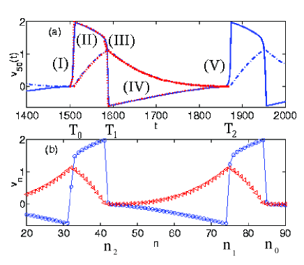
Figure 2: Wave train for FHN: (a) Temporal profiles of $v_{n}(t)$ (solid) and $w_{n}(t)$ (dashed-dotted), compared to their asymptotic reconstruction (dotted); (b) Spatial profiles of $v_{n}$ (circles) and $w_{n}$ (triangles). Parameter values are $a=0.1$, $b=0.5$, $D=0.02$, $\lambda=0.01$, $w=0.002$.

Having described the reduced dynamics of wave front solutions of bistable equations in Section 2.1, we are ready to predict asymptotically the speed and shape of wave trains for (1)-(2) in the limit $\lambda\rightarrow 0^{+}$.

Discrete wave trains have the form $v_{n}(t)=V(n-ct)$, $w_{n}(t)=W(n-ct)$. $V$ and $W$ are real functions of a real variable $z=n-ct$. Note that $z$ takes on continuous values and not discrete values like the variable $n$. Thus $V$ and $W$ are perfectly determined once their speed $c$, period $L$ and continuous profiles $V(z)$ and $W(z)$, $z\in[0,L]$, are known. If we fix $n$, the trajectories $v_{n}(t)=V(n-ct)$, $w_{n}(t)=W(n-ct)$ are periodic in the continuous variable $t$ and have a well defined temporal period $L/c$. Thus, once we compute the speed $c$ and the temporal profiles $v_{n}(t),w_{n}(t)$ as functions of $t$ for fixed $n$, the wave train profiles $V$ and $W$ and their period $L$ are known. If we fix $t$ and vary the discrete spatial variable $n$, the situation is different. The spatial structure of the wave train at each fixed time $t$ is given by $v_{n}=V(n-ct)$ and $w_{n}=W(n-ct)$. The points contained in a period satisfy $0\leq n-ct\leq L$, that is, $ct\leq n\leq L+ct$. As time grows, the discrete points ’travel’ along the continuous wave profile and are transferred from one period to the next. The number of integers $n$ one can fit in an interval of length $L$ is the integer part of $L$.

There are no rigorous existence results for wave train solutions of (1)-(2). Assuming that wave trains do exist, we shall use the separation of time scales $\lambda$ to find an approximate reconstruction of the temporal wave train profiles by matched asymptotic expansions at zeroth order as $\lambda\rightarrow 0^{+}$. A description of matched asymptotic expansions can be found in [18] or in the more elementary reference [3].

For $D$ small, numerical solutions show that wave train trajectories should be composed of regions of smooth variation of $(v_{n},w_{n})$ on the slow time scale $T=\lambda t,$ separated by sharp interfaces in which $v_{n}$ varies rapidly in the fast time scale $t$, see Figure 2. The reference time in our construction of trajectories will be the slow time $T.$

For $n$ fixed, we may distinguish four stages in one time period of the wave train solutions $(v_{n}(T;\lambda),w_{n}(T;\lambda))$. At each stage, a reduced description holds:

• Leading edge (I) in Figure 2 (a). The variable $v_{n}$ evolves abruptly in the fast time scale $\mbox{\~{t}}={T-T_{0}\over\lambda}\in(-\infty,\infty)$. To leading order:

  $$\begin{array}[]{l}{dv_{n}\over d\mbox{\~{t}}}=D(v_{n+1}-2v_{n}+v_{n-1})+f(v_{n},w_{n}),\quad{dw_{n}\over d\mbox{\~{t}}}=0.\end{array}$$ (10)

  Thus, $w_{n}=w$ is a constant and $v_{n}$ is the temporal profile of the wave front solution of (8) which joins $z_{1}(w)$ and $z_{3}(w)$. This front propagates with a speed $c_{+}(w,D)$ when $w\in(w_{-},w_{c-}(D))$.

• Peak. This is region (II) in Figure 2 (a). Here $v_{n}$ varies smoothly on the slow time scale $T$. Thus, we may set $D=0$, obtaining the reduced problem $f(v_{n},w_{n})=0,$ ${dw_{n}\over dT}=g(v_{n},w_{n})$. Matching the peak to the leading edge at zeroth order, we see that $v_{n}$ must lie in the third branch of roots of the cubic function: $v_{n}=z_{3}(w_{n}).$ Then, for $T_{0}<T<T_{1}(w,\overline{w})$:

  $${dw_{n}\over dT}=g(z_{3}(w_{n}),w_{n}),$$ (11)

  $$T_{1}(w,\overline{w})=T_{0}+\int_{w}^{\overline{w}}\!{ds\over g(z_{3}(s),s)},$$ (12)

  in which $w_{n}(T_{0})=w$ and $w_{n}(T_{1})=\overline{w}$ (to be calculated later).

  The matching conditions at $T=T_{0}$ for the reduced descriptions of the peak and the leading front are :

  $$\begin{array}[]{l}z_{3}(w_{n}^{(II)}(T))-v_{n}^{(I)}({T-T_{0}\over\lambda})\ll 1,\quad w_{n}^{(II)}(T)-w\ll 1,\end{array}$$ (14)

  as $\lambda\to 0+$ in the overlap region $\lambda\ll T-T_{0}\ll 1$. The superscripts (I), (II) … refer to the region and the reduced description we are using. The uniform approximations of the profiles in stages (I)-(II) are:

  $$\begin{array}[]{l}v_{n}^{unif}=v_{n}^{(I)}({T-T_{0}\over\lambda})+z_{3}(w_{n}^{(II)}(T))-z_{3}(w),\quad w_{n}^{unif}=w_{n}^{(II)}(T).\end{array}$$ (16)

• Trailing wave front. The peak is followed by another region of fast variation of $v_{n}$, corresponding to (III) in Figure 2 (a). Again, (10) holds to leading order, on the new time scale $\mbox{\~{t}}={T-T_{1}\over\lambda}\in(-\infty,\infty)$. Thus, $w_{n}=\overline{w}$ is a constant and $v_{n}$ is the temporal profile of the wave front solution of (10) with $w_{n}=\overline{w}$ which joins $z_{3}(\overline{w})$ and $z_{1}(\overline{w})$. This front propagates with a speed $c_{-}(\overline{w},D)$ when $\overline{w}\in(w_{c+}(D),w_{+})$. If the wave train is to move rigidly, $\overline{w}$ must be selected in such a way that the trailing front travels with speed $c_{-}(\overline{w},D)=c_{+}(w,D)=c$.

  The matching conditions for the reduced descriptions of the peak and the trailing front at $T=T_{1}$ are:

  $$\begin{array}[]{l}z_{3}(w_{n}^{(II)}(T))-v_{n}^{(III)}({T-T_{1}\over\lambda})\ll 1,\quad-w_{n}^{(II)}(T)+\overline{w}\ll 1,\end{array}$$ (18)

  as $\lambda\to 0+$ in the overlap region $\lambda\ll T_{1}-T\ll 1$. The uniform approximations of the profiles in regions (I)-(III) are:

  $$\begin{array}[]{l}v_{n}^{unif}=v_{n}^{(III)}({T-T_{1}\over\lambda})+v_{n}^{(I)}({T-T_{0}\over\lambda})+z_{3}(w_{n}^{(II)}(T))-z_{3}(w)-z_{3}(\overline{w}),\\ w_{n}^{unif}=w_{n}^{(II)}(T).\end{array}$$ (21)

• Tail. The last part of the period is region (IV) in Figure 2 (a). Here, $v_{n}$ varies smoothly on the slow time scale $T$, and $D$ can be neglected. The reduced problem is $f(v_{n},w_{n})=0,$ ${dw_{n}\over dT}=g(v_{n},w_{n})$. Matching the tail to the trailing wave front at zeroth order, we see that $v_{n}$ must lie in the first branch of roots: $v_{n}=z_{1}(w_{n}).$ Then, for $T_{1}<T<T_{2}(w,\overline{w})$:

  $${dw_{n}\over dT}=g(z_{1}(w_{n}),w_{n}),$$ (22)

  $$T_{2}(w,\overline{w})=T_{1}+\int_{\overline{w}}^{w}\!{ds\over g(z_{1}(s),s)},$$ (23)

  in which $w_{n}(T_{1})=\overline{w}$ and $w_{n}(T_{2})=w=w_{n}(T_{0})$, if the wave train is to move rigidly. In this way, we conclude the description of one temporal period and guarantee that the end of its tail can be matched to the following (identical) period. Notice that the integral (23) diverges when $w\geq w^{0}$ due to a singularity at the equilibrium value $w^{0}$. Thus, the range of $w$ for which we can find wave trains is restricted to $(w^{0},w_{c-}(D)).$

  The matching conditions for the reduced descriptions of the tail and the trailing front at $T=T_{1}$ are:

  $$\begin{array}[]{l}v_{n}^{(III)}({T-T_{1}\over\lambda})-z_{1}(w_{n}^{(IV)}(T))\ll 1,\quad-w_{n}^{(IV)}(T)+\overline{w}\ll 1,\end{array}$$ (25)

  as $\lambda\to 0+$ in the overlap region $\lambda\ll T-T_{1}\ll 1$. The uniform approximations of the profiles in regions (III)-(IV) are:

  $$\begin{array}[]{l}v_{n}^{unif}=v_{n}^{(III)}({T-T_{1}\over\lambda})+z_{1}(w_{n}^{(IV)}(T))-z_{1}(\overline{w}),\quad w_{n}^{unif}=w_{n}^{(IV)}(T).\end{array}$$ (27)

  In a similar way, the end of the tail should be matched to the leading edge (region (V)) of the next period at $T_{2}$.

A uniform approximation to the temporal profile in a whole period is obtained as follows. Let $\chi(a,b)$ be the indicator function, equal to $1$ if $a\leq T\leq b$ and $0$ otherwise. Then, for $T_{0}\leq T\leq T_{2}$:

$$\begin{array}[]{l}v_{n}^{unif}(T)=\big{[}v_{n}^{(III)}({T-T_{1}\over\lambda})\!+\!v_{n}^{(I)}({T-T_{0}\over\lambda})\!+\!z_{3}(w_{n}^{(II)}(T))\!-\!z_{3}(w)\!-\!z_{3}(\overline{w})\big{]}\chi(T_{0},T_{1})\\ \quad\quad\quad\;\;+\big{[}v_{n}^{(III)}({T-T_{1}\over\lambda})\!+\!v_{n}^{(V)}({T-T_{2}\over\lambda})\!+\!z_{1}(w_{n}^{(IV)}(T))\!-\!z_{1}(w)\!-\!z_{1}(\overline{w})\big{]}\chi(T_{1},T_{2}),\\ w_{n}^{unif}(T)=w_{n}^{(II)}(T)\chi(T_{0},T_{1})+w_{n}^{(IV)}(T)\chi(T_{1},T_{2}).\end{array}$$ (31)

This construction yields a family of wave trains parametrized by the values $w\in(w^{0},w_{c-}(D))$ for which there exists $\overline{w}=\overline{w}(w)\in(w_{c+}(D),w_{+})$ satisfying $c_{-}(\overline{w},D)=c_{+}(w,D)=c$.

In Figure 2 (a), we have superimposed the approximate temporal profile provided by our matched asymptotic expansions and the numerically calculated profile. They are indistinguishable. Notice that, for small $D$, the leading and trailing wave fronts can be accurately computed using one active point (see section 2.1 or [8]):

$${dv_{n}\over d\mbox{\~{t}}}=D(z_{3}(w)-2v_{n}+z_{1}(w))+f(v_{n},w),$$ (32)

$${dv_{n}\over d\mbox{\~{t}}}=D(z_{3}(\overline{w})-2v_{n}+z_{1}(\overline{w}))+f(v_{n},\overline{w}).$$ (33)

In the true time scale $t={T\over\lambda}$, the temporal period of the wave train is asymptotic to $\big{(}T_{2}(w)-T_{0}\big{)}/\lambda$ (the duration of the fast stages (I) and (III) is ignored).

Having calculated the temporal profiles $v_{n}(t),w_{n}(t)$ of a wave train and its velocity $c$, the wave train profiles $V$, $W$ are known: $V(z)=v_{n}({n-z\over c})$ and $W(z)=w_{n}({n-z\over c})$, $z=n-ct$. Their period is now asymptotic to $c_{+}(w)\big{(}T_{2}(w)-T_{0}\big{)}/\lambda$. The number of points $L(w)$ in the wave length of the wave train is essentially the integer part of the wave length. Figure 2 (b) illustrates that, at a fixed time $t$:

• the leading front of one spatial period is located at a point $n_{0}$, where $w_{n_{0}}(t)\sim w$,

• its trailing front is located at a point $n_{1}$, such that $w_{n_{1}}(t)\sim\overline{w}$,

• the end of our spatial period and the beginning of the next one is located at a point $n_{2}$, where $w_{n_{2}}(t)\sim w$.

Then, $L(w)=n_{0}-n_{2}$ is approximately the integer part of $c_{+}(w)\big{(}T_{2}(w)-T_{0}\big{)}/\lambda$. Notice that the number of points inside the leading and trailing fronts of each period can be ignored in the discrete limit $D\ll 1$. The number of points in the peak $L_{1}(w)=n_{0}-n_{1}$ is asymptotic to the integer part of $c_{+}(w)\big{(}T_{1}(w)-T_{0}\big{)}/\lambda$ and the number of points in the tail $L_{2}(w)=n_{1}-n_{2}$ is asymptotic to the integer part of $c_{+}(w)\big{(}T_{2}(w)-T_{1}(w)\big{)}/\lambda$. Our construction is consistent only when $L_{1}(w)\geq 1$. This provides an estimate of the critical value $\lambda_{c}(D)$ above which propagation fails. Nevertheless, near the thresholds for propagation failure, the approximation described in this section has to be corrected. This is explained in more detail in Section 4.

2.3 Solitary pulses

A wave train becomes a traveling pulse when its spatial period tends to infinity, which occurs as $w\rightarrow w^{0}$. Pulses are the fastest waves of the family. In the asymptotic description of the temporal profile of a pulse we distinguish five regions:

• In front of the pulse, the profile is at equilibrium: $v_{n}\sim v^{0}$, $w_{n}\sim w^{0}$.

• The leading edge of the pulse is a wave front solution of (10) with $w_{n}=w^{0}$, which joins $z_{1}(w^{0})=v^{0}$ and $z_{3}(w^{0})$. This front propagates with a definite speed $c=c_{+}(w^{0},D)$.

• In the transition between fronts, $v_{n}=z_{3}(w_{n})$, ${dw_{n}\over dT}=g(z_{3}(w_{n}),w_{n})$ and $w_{n}$ evolves from $w^{0}$ at $T_{0}$ to $\overline{w}^{0}$ at $T_{1}$.

• The trailing wave front is the wave front solution of (10) with $w_{n}=\overline{w}^{0}$, which joins $z_{3}(\overline{w}^{0})$ and $z_{1}(\overline{w}^{0})$. $\overline{w}^{0}$ is now selected in such a way that this front travels with speed $c=c_{-}(\overline{w}^{0},D)=c_{+}(w^{0},D)$.

• In the pulse tail, $v_{n}=z_{1}(w_{n})$, ${dw_{n}\over dT}=g(z_{1}(w_{n}),w_{n})$ and $w_{n}$ evolves from $\overline{w}^{0}$ to $w^{0}$.

The number of points between fronts $L_{1}(w^{0})$ is again asymptotic to the integer part of of $c_{+}(w^{0})(T_{1}(w^{0})-T_{0})/\lambda$. The number of points in the tail is infinite, since the integral $\int_{\overline{w}^{0}}^{w^{0}}{ds\over g(z_{1}(s),s)}$ diverges. However, we can predict how long does it take for the tail to get sufficiently close to $v^{0}=z_{1}(w^{0})$ by using $\int_{\overline{w}^{0}}^{w^{0}-\epsilon}{ds\over g(z_{1}(s),s)},$ with $\epsilon>0$ instead.

3 Periodic firing of waves at boundaries

When an excitable medium is periodically excited, we expect propagation of signals in form of wave trains. We will see here that the periodic wave train solutions constructed in Section 2 allow to describe propagation due to periodic firing at a boundary in the spatially discrete FHN and ML models.

3.1 FitzHugh-Nagumo

The FitzHugh-Nagumo (FHN) model is a crude simplification of (1)-(2) that sets $f(v,w)=h(v)-w$ with $g$ linear. Typically, $h$ is chosen to be a cubic polynomial, say $h(v)=v(v-a)(2-v)$. We get:

$${dv_{n}\over dt}\!=\!D(v_{n+1}\!-\!2v_{n}\!+\!v_{n-1})\!+\!v_{n}(v_{n}\!-\!a)(2\!-\!v_{n})\!-\!w_{n},$$ (34)

$${dw_{n}\over dt}=\lambda(v_{n}-bw_{n}).$$ (35)

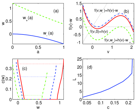
Figure 3: For FHN: (a) Critical curves for cubic shape; (b) Change of symmetry in the source as $w$ increases from $w_{-}$ to $w_{+}$; (c) Speed curves when $D=0.1$ for $a=0.55$ (solid), $a=0.3$ (dashed), $a=0.1$ (dashed-dotted); (d) Dispersion law $L(c)$ for $D=0.1$ and $\lambda=0.05$.

When $a\in(0,1)$, this system is excitable provided $b$ is not too large, as illustrated in Figure 1(a). The unique stationary state is $(v^{0},w^{0})=(0,0)$. As Figure 3(b) shows, the source $v(v-a)(2-v)-w$ is bistable when $w\in(w_{-}(a),w_{+}(a))$. The curves $w_{-}(a)$, $w_{+}(a)$ are plotted in Figure 3(a). The reduced equation (34) with $w_{n}=w$ has decreasing (resp. increasing) traveling wave front solutions moving with speed $c_{+}(w)$ (resp. $c_{-}(w)$) when $w\in(w_{-}(a),w_{c-}(a,D))$ (resp. $w\in(w_{c+}(a,D),w_{+}(a))$). Figure 3(c) depicts the speed curves $c(w)$ for different values of $a$. The left branches represent $c_{+}(w)$ and the right branches $c_{-}(w)$. The horizontal dotted lines join $c_{+}(0)$ with $c_{-}(\overline{w}^{0})$, selecting the value $\overline{w}^{0}$ for the trailing front in the construction of pulses.

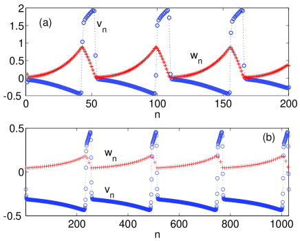
Figure 4: (a) Wave train for FHN when $D=0.1$, $a=0.3$ $\lambda=10^{-2}$, $w=0.02$, $c=0.18$; (b) Wave train for ML with $D=1$, $\lambda=10^{-3}$, $w=0.045$, $c=0.54$.

Wave trains are found when $w\in(0,w_{c-}(a,D))$. They are slower than pulses. Figure 4(a) shows a wave train for $a=0.3$, $w=0.02$ and $\lambda=0.01$. It has been generated by solving (34)-(35) with initial data $v_{n}(0)=2$, $n=1,...,10$, $v_{n}(0)=0$, $n>10$, $w_{n}(0)=0.01$ and a periodic excitation at the left boundary. More precisely, we have used boundary conditions of the form:

$$v_{0}(t)=\left\{\begin{array}[]{ll}2&t\in[0,\rho T]+kT,\\ 0&t\in(\rho T,T]+kT,\end{array}\right.$$ (36)

with $k\in I\!\!N$, $0<\rho<1$. Our theory predicts $c=0.18$, $L_{1}=9$ and $L_{2}=45$, close to the numerically measured values $c=0.175$, $L_{1}=10$, $L_{2}=46$. For $w=0.002$, our theory predicts $c=0.2$. When $\lambda=0.05$, $L_{1}=2$ and $L_{2}=14$. Numerically, we find $c=0.16$, $L_{1}=1-2$, $L_{2}=13-14$.

We have plotted the dispersion relation $L(c)$ ($L(w)$ against $c_{+}(w)$) for our asymptotic family of wave trains in Figure 3(d). Note that $L^{\prime}(c)>0$. Our numerical tests with periodic boundary conditions starting from initial conditions which are near the shape asymptotically predicted for these wave trains suggest their stability. For continuous systems like (3), Maginu [19] proved stability of wave trains under the condition $L^{\prime}(c)>0$. Our numerical experiments suggest that a similar stability criterion could be established for wave trains in discrete systems.

3.2 Morris-Lecar dynamics

The non dimensional Morris-Lecar (ML) model [22] is:

$${dv_{n}\over dt}=D(v_{n+1}-2v_{n}+v_{n-1})+f(v_{n},w_{n})-2I,$$ (37)

$${dw_{n}\over dt}={\lambda}\cosh({v_{n}-{V}_{3}\over 2{V}_{4}})\big{[}1+\tanh({v_{n}-{V}_{3}\over{V}_{4}})-2w_{n}\big{]},$$ (38)

where the index $n$ denotes the $n$-th site and:

$$f(v,w)=2w(v-{V}_{K})+2{g}_{L}(v-{V}_{L})+{g}_{Ca}\big{[}1+\tanh({v-{V}_{1}\over{V}_{2}})\big{]}(v-1).$$ (39)

$v_{n}$ is the ratio of membrane potential to a reference potential and $w_{n}$ is the fraction of open $K^{+}$ channels. The time scale is ${\overline{g}_{K}\over 2C_{m}}$, $\overline{g}_{K}$ being the $K^{+}$ conductance and $C_{m}$ the membrane capacitance. System (37)-(38) is a reduced version of the full Morris-Lecar model [22], which involves one more fast variable $m_{n}$. Typical values for the parameters can be taken from experiments [22]. In our numerical tests we have used:

$$\begin{array}[]{|c|c|c|c|c|c|c|c|c|}\hline\cr g_{Ca}&g_{L}&I&V_{K}&V_{L}&V_{1}&V_{2}&V_{3}&V_{4}\\ \hline\cr 0.5&0.25&0.0625&-0.7&-0.5&0.1&0.15&-0.01&0.145\\ \hline\cr\end{array}$$ (42)

System (37)-(38) exhibits a rich dynamical behavior depending on its nullclines. Figure 1(b) shows two possibilities. For $I=0.375$, the system develops self-oscillations. This behavior will be discussed in Section 5. For $I=0.0625$, the system is excitable. Figure 5(a) illustrates the change of symmetry in the source $f(v,w)$ as $w$ increases from $w_{-}$ to $w_{+}$. The thresholds for wave front propagation $w_{c-}(D)$ and $w_{c+}(D)$ are depicted in Figure 5(b). Note that the size of the pinning interval grows as $D$ decreases. The curves $c_{-}(w)$ and $c_{+}(w)$ representing the speeds of the wave front solutions of the reduced bistable equation for this problem with $D$ fixed are shown in Figure 5(c). We have plotted the dispersion relation $L(c)$ ($L(w)$ against $c_{+}(w)$) for our asymptotic family of wave trains in Figure 5(d). Again, $L^{\prime}(c)>0$ and this branch of wave trains is expected to be stable for the dynamics (37)-(38).

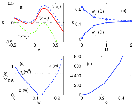
Figure 5: For ML: (a) Change of shape in $f(v,w)$; (b) Pinning thresholds $w_{c-}(D)$ and $w_{c+}(D)$; (c) Speed curves $c_{-}(w)$ and $c_{+}(w)$ with $D=1$; (d) Dispersion law $L(c)$ for $D=1$ and $\lambda=10^{-3}$.

We have generated a variety of wave trains using the asymptotic prediction as initial datum and periodic boundary conditions. These numerical solutions agree reasonably well with the asymptotic description given in Sections 2.2. Figure 4(b) shows a wave train for $D=1$, $\lambda=10^{-3}$, $w=0.045$, $c=0.54$. For $w=0.045$, the predicted speed is $c=0.54$. When $\lambda=10^{-3}$, we predict a peak width $L_{1}\sim 19$ and a tail width $L_{2}\sim 256$. The numerically measured parameters are $c\sim 0.55$, $L_{1}\sim 18$ and $L_{2}\sim 250$.

The basin of attraction of wave trains is rather small and their existence depends crucially on the boundary conditions we employ. There are no wave trains if we replace the periodic boundary conditions by Dirichlet or Neumann boundary conditions. With periodic boundary conditions, wave trains fail to be formed if $w_{n}(0)$ is near the equilibrium value $w^{0}$. In such a case, the initial condition evolves toward a solitary pulse instead of a wave train.

Pulses are more robust. They can be generated using different initial data and boundary conditions. For instance, we can chose step-like initial data $v_{n}(0)$, climbing from $v^{0}$ to a value close to $z_{3}(w^{0})$. For $w_{n}(0)$ we may take a perturbation of $w^{0}$, as long as $w_{n}(0)$ is near the value $\overline{w}^{0}$ in the trailing front of the step. These initial conditions evolve into pulses, regardless of whether we are using Dirichlet or periodic boundary conditions. When $D=0.1$, our asymptotic construction predicts pulses with speed $c\sim 0.075$. Setting $\lambda=10^{-4}$, the predicted peak width is $L_{1}\sim 35$. The tail reaches the value $w^{0}-\epsilon$, $\epsilon=10^{-2}$, for $L_{\epsilon}\sim 455$. Again, these values describe accurately the numerically constructed pulses.

We observe that the profiles of wave trains and pulses differ slightly depending on whether their speeds are large or small. Fast waves have smooth temporal profiles and advance smoothly. Slow waves develop a sequence of steps in the leading and trailing fronts. Their motion is ’saltatory’. Figure 6 shows the spatial and temporal profiles of a slow wave train when $D=1$, $\lambda=10^{-5}$, $w=0.108$ and $c=0.04$. The values $w$ and $\overline{w}$ are close to the thresholds $w_{c-}(D)$ and $w_{c+}(D)$, that is, near the depinning transitions [8] for the bistable equation (8). This is the reason for the appearance of the steps that can be appreciated in Figure 6(b). Wave trains and pulses are always ’slow’ when $D$ is near the threshold $D_{c}$ for propagation failure. For our parameter values, $w^{0}$ is near the threshold $w_{c-}(D)$ when $D\sim 0.076$, and the profile of the pulses and wave trains are staircase like.

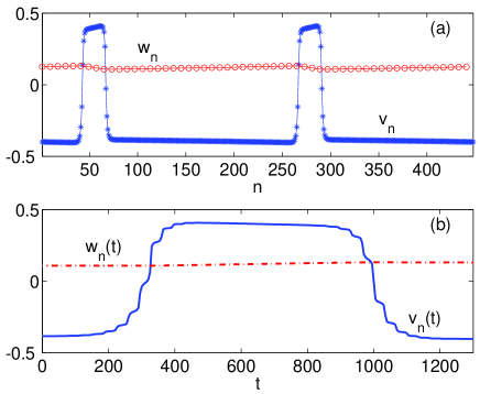
Figure 6: Slow wave trains for Morris-Lecar: (a) spatial profile at a fixed time $t$, (b) detail of the steps in the temporal profile. Parameter values are $D=1$, $\lambda=10^{-5}$, $w=0.108$ and $c=0.04$.

4 Propagation failure

In both discrete and continuous models, wave trains and pulses disappear as $\lambda$ increases beyond certain thresholds. However, the way in which these waves disappear can be rather different. In continuous models, the height of the peak of a pulse or a wave train decreases as $\lambda$ increases and, eventually, waves cease to propagate. In discrete models, new modes of propagation failure arise depending on the value of $D$. Unlike the continuous case, waves also fail to propagate when $D$ is smaller than a critical value $D_{c}$. Figure 7 depicts the critical separation of time scales $\lambda_{c}(D)$ for FHN as a function of $D$. We distinguish three regions: small $D$ (highly discrete limit), large $D$ (continuum limit) and intermediate $D$. For the parameter values selected in Figures 7-10, these regions are approximately $D_{c}<D\leq 0.01$, $0.01<D<0.3$ and $0.3\leq D$. Figures 7 (b) and (c) zoom in the highly discrete and the intermediate regions.

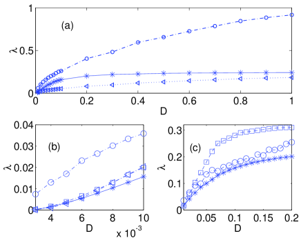
Figure 7: Numerically measured $\lambda_{c}(D)$ (asterisks) compared to: (a) the upper bound $\lambda_{c}(D)^{+}$ (circles) and the lower bound $\lambda_{c}(D)^{-}$ (triangles); (b) and (c), the upper bound $\lambda_{c}(D)^{+}$ (circles), the numerically measured $\lambda_{0}(D)$ (squares) and its asymptotic prediction (48) (triangles). Parameter values for FHN are $a=0.1$, $b=0.5$, $k=5$.

Figure 8: Pulses near $D_{c}$ and $\lambda_{c}(D)$: (a) Spatial profile and (b) Temporal profile (solid line) when $D=0.004$ and $\lambda=0.0054$; (c) Spatial profile and (d) Temporal profile (solid line) when $D=0.009$ and $\lambda=0.013$. In (b) and (d), dashed lines represent the temporal profiles of the slow variable. Dashed-dotted and dotted lines are the solutions of the reduced equations (46)-(47). Other parameter values for FHN are $a=0.1$ and $b=0.5$.

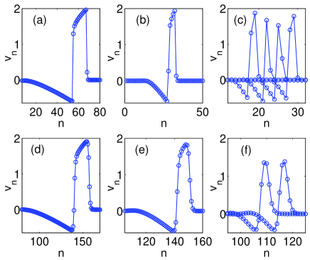
Figure 9: Pulses for FHN with $a=0.1$,$b=0.5$ and increasing $\lambda$. When $D=0.03$: (a) $\lambda=0.01$, (b) $\lambda=0.03$, (c) $\lambda=0.065$. When $D=0.7$: (d) $\lambda=0.05$, (e) $\lambda=0.1$, (f) $\lambda=0.237$.

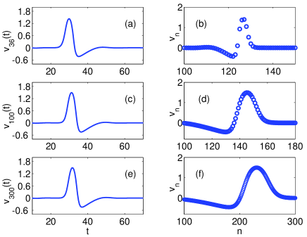
Figure 10: Pulses for FHN near $\lambda_{c}(D)$ with $a=0.1$,$b=0.5$ and increasing $D$. Temporal profiles when (a) $D=1$, (c) $D=10$, (e) $D=100$. The small oscillation in the tail indicates that $(0,0)$ has just become a spiral point. Spatial profiles when (b) $D=1$, (d) $D=10$, (f) $D=100$.

Figure 8 illustrates the shape of pulses for FHN when $D$ is near $D_{c}$. For $\lambda$ close to $\lambda_{c}(D)$, the height of the pulses has not decreased and remains near its maximum value $2$. The width of the pulses does not vanish either. Moreover, it is quite large near the critical coupling $D_{c}$. Close to $\lambda_{c}(D)$, the peak contains $3$ points if $D=0.009$. This number increases to $8$ points when $D=0.004$. For $D=0.003,$ we reach $30$ points. The number of points in the peak of a propagating pulse near the critical time scale separation $\lambda_{c}(D)$ seems to increase as $D$ approaches $D_{c}$. Then, why do pulses fail to propagate? Near $D_{c}$ the leading edge advances in the slow ’saltatory’ manner typical of wave fronts at the depinning transition [8]. Then, the separation of time scales described in earlier Sections becomes blurred. Both variables, $v_{n}$ and $w_{n}$ change as the leading front moves. For $D$ fixed, and as $\lambda$ increases, the leading edge becomes pinned and ceases to propagate at a critical value of $\lambda$. Thus, in the highly discrete region, waves fail to propagate at $\lambda_{c}(D)$ due to the pinning of the leading edge.

For intermediate values of $D$, the peak of propagating pulses near the critical time scale separation $\lambda_{c}(D)$ contains one point, see Figure 9 (c). The temporal profiles of these pulses show a peak with a narrow trapezoidal shape. Thus, their spatial profiles change noticeably as the pulse moves, showing the configurations with variable height depicted in Figure 9 (c). The reason for propagation failure in this region is the vanishing width of the peaks as $\lambda$ increases.

For larger $D$, the mechanism of propagation failure as $\lambda$ grows is related to the decreasing height of the pulses, as in the continuum limit. In fact, the profiles and speeds of the pulses near $\lambda_{c}(D)$ resemble the profile and speed of the pulse solutions of (3) near the critical time scale separation $\lambda_{c}$ for the continuous problem, as shown by Figures 9 (f) and 10. As $D$ grows, more and more points accumulate in the leading and trailing fronts (see Fig. 10) and propagation fails before the top of the pulse is reduced to one point.

In this Section, we exploit (and correct) the predictions provided by the asymptotic construction of travelling wave trains and pulses carried out in Section 2 to characterize the critical coupling $D_{c}$ and the critical separation of time scales for propagation $\lambda_{c}(D)$. First, we consider travelling pulses and then we turn to wave trains.

4.1 Propagation failure for pulses

For a fixed $D$, the asymptotic construction in Section 2.3 yields upper and lower bounds on the critical value $\lambda_{c}(D)$ above which propagation of pulses fails, as a function of $D.$ Moreover, we find an asymptotic prediction of $\lambda_{c}(D)$ for small $D$, which agrees reasonably with numerical measurements. Prior to this work, the only work in this direction is contained in the paper by Chen and Hastings [11], who found rather coarse upper bounds on the separation of time scales for a particular class of sources that excludes FHN and most realistic sources.

An upper estimate $\lambda_{c}(D)^{+}$ on $\lambda_{c}(D)$ is found observing that our asymptotic construction is consistent when the peak has one or more points: $L_{1}(w^{0},D,\lambda)\geq 1$. Therefore:

$$\lambda\leq\lambda_{c}(D)\leq\lambda_{c}(D)^{+}=c_{+}(w^{0},D)\int_{w^{0}}^{\overline{w}(w^{0},D)}{ds\over g(z_{3}(s),s)}.$$ (43)

On the other hand, numerical solutions show that pulses fail to propagate when $L_{1}(w^{0},D,\lambda)$ is smaller than a certain number of points $k(D)$. Once $k(D)$ is determined:

$$\lambda\geq\lambda_{c}(D)^{-}={c_{+}(w^{0},D)\over k(D)}\int_{w^{0}}^{\overline{w}^{0}(w^{0},D)}{ds\over g(z_{3}(s),s)}$$ (44)

yields a lower bound $\lambda_{c}(D)^{-}$ for $\lambda_{c}(D)$. Without a theory to predict $k(D)$, our choice $k(D)=5$ for $D\in(0.01,1)$ in Figure 7 (a) is empirical.

Figure 7(a) compares the numerically calculated $\lambda_{c}(D)$ with the upper and lower bounds $\lambda_{c}(D)^{\pm}$ for the FitzHugh-Nagumo model. The numerical approximation of $\lambda_{c}(D)$ is obtained as follows. We solve the initial value problem (34)-(35) starting from the equilibrium state $(0,0)$ and excite the left boundary for a large enough time $T$: $v_{0}(t)=2\chi(0,T)$, $w_{0}(t)=0$, $t>0$. If a pulse is successfully generated, we increase $\lambda$ slightly. The process stops when we reach a value of $\lambda$ for which pulses cease to be formed.

As Figure 7(a) shows, bounds (43)-(44) are not sharp. There are several reasons for this. First, the minimum number of points in the peak before propagation failure changes with $D$. Second, as $\lambda$ grows the height of the propagating pulses diminishes and our asymptotic construction loses precision. Third, near the critical coupling $D_{c}$, the reduced bistable equation (8) does not describe accurately the speed of the leading front. The relevance of these three factors varies with $D$. We will improve our predictions of $\lambda_{c}(D)$ by a more precise study of the three regions mentioned before: highly discrete, continuous and intermediate.

4.1.1 Highly discrete limit

In the highly discrete limit, $D\ll 1$, $w^{0}\sim w_{c-}(D)$ and we are near the depinning transition of wave fronts characterized by a saltatory motion of active points, see Section 2.1. During the long time intervals between abrupt jumps of the saltatory motion, $w_{n}$ can change appreciably and the reduced equation for the motion of the leading edge of pulses:

$${dv_{n}\over dt}=D(v_{n+1}-2v_{n}+v_{n-1})+f(v_{n},w^{0})$$ (45)

is no longer accurate. Instead of (32) with $w=w^{0}$, the evolution of the active point is governed now by:

$${dv\over dt}=D(z_{3}(w)-2v+z_{1}(w))+f(v,w),$$ (46)

$${dw\over dt}=\lambda g(v,w).$$ (47)

Figures 8 (b) and (d) compare solutions of (46)-(47), represented by dashed lines, with the temporal profile of the pulses. The leading edges are accurately described.

As we increase $\lambda$, we find a critical value $\lambda_{0}(D)$ at which trajectories of (46)-(47) jumping from a neighborhood of $(v^{0},w^{0})=(z_{1}(w^{0}),w^{0})$ to a neighborhood of $(z_{3}(w^{0}),w^{0})$ cease to exist. We obtain a first impression about $\lambda_{0}(D)$ by examining the phase plane in Figure 11. System (46)-(47) has an equilibrium point. For $\lambda$ small, the equilibrium point is a node and trajectories starting at $(z_{1}(w^{0}),w^{0})$ reach a neighborhood of $(z_{3}(w^{0}),w^{0})$, as shown by the dashed lines in Figure 11 (a). As $\lambda$ grows, it becomes a spiral point. Trajectories originating at $(z_{1}(w^{0}),w^{0})$ wrap around the equilibrium point, without reaching $(z_{3}(w^{0}),w^{0})$, see Figure 11 (b). If we compute the value of $\lambda$ at which the equilibrium changes type, we find an approximate value for $\lambda_{0}(D)$. This approximation happens to be quite poor: it is almost constant for $D$ small.

A better prediction of $\lambda_{0}(D)$ is found by calculating two characteristic times. Suppose $w$ does not depart appreciably from $w^{0}\approx w_{c-}(D)$. The depinning analysis explained in [8] shows that the quiescent period between successive jumps in saltatory motion is $t_{v}\sim{\pi\over\sqrt{\alpha\beta(w^{0}-w_{c-}(D))}}$. During this quiescent period, $v\sim s_{0}$, $s_{0}$ being a value between $z_{1}(w^{0})$ and $z_{2}(w^{0})$ (see Section 2.1). Suppose on the contrary that $\lambda$ is so large that $w$ increases from $w^{0}$ to $w_{c-}(D)$ while $v\sim s_{0}$. This occurs in a time $t_{w}=\int_{w^{0}}^{w_{c-}(D)}dw/\lambda g(s_{0},w)$. If $t_{v}\ll t_{w}$, saltatory motion of pulses can proceed. In the opposite limit, $t_{v}\gg t_{w}$, $w$ evolves towards the equilibrium value of (46)-(47) and the pulse stops. The crossover value at which $t_{v}\sim t_{w}$ yields the estimated critical value $\lambda_{0}(D)$:

$$\lambda_{0}(D)\sim{\sqrt{\alpha\beta(w^{0}-w_{c-}(D))}\over\pi}\int_{w^{0}}^{w_{c-}(D)}{dw\over g(s_{0},w)}.$$ (48)

For FHN, $w^{0}=0$ and $\int_{0}^{w_{c-}(D)}{dw\over s_{0}-bw}=-{1\over b}\ln(1-b{w_{c-}(D)\over s_{0}})\sim{w_{c-}(D)\over s_{0}}$. Thus, $\lambda_{0}(D)\sim{w_{c-}(D)\over s_{0}}{\sqrt{\alpha\beta(-w_{c-}(D))}\over\pi}$. Figure 7 (b) compares $\lambda_{c}(D)$ with the numerically measured value of $\lambda_{0}(D)$, our asymptotic prediction (48) and the upper bound $\lambda^{+}(D)$. Now, this upper bound is computed using the approximation of the speed provided by (46)-(47) instead of the speed of the wave front solution of (8). Notice the good agreement between $\lambda_{c}(D)$ and $\lambda_{0}(D)$ for small $D$.

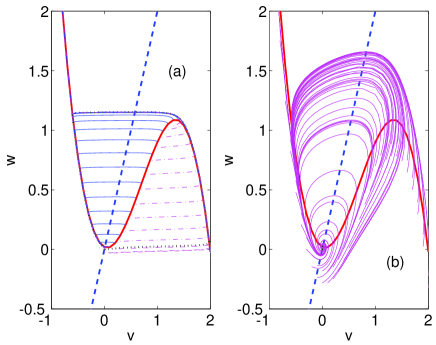
Figure 11: Phase plane for the reduced system (46)-(47): (a) $\lambda=0.01$, (b) $\lambda=0.1$. Parameter values for FHN are $D=0.01$, $a=0.1$, $b=0.5$.

4.1.2 Intermediate region and Continuous limit

In the intermediate region, the peak of the pulses contains one point near $\lambda_{c}(D)$ and the upper bound $\lambda^{+}(D)$ provides a good estimate of the critical threshold. Formula (43) is more accurate when we replace the speed of the wave front solutions of the reduced bistable equation (used in Figure 7 (a)) by the speed found solving numerically (46)-(47) (used in Figure 7 (c)).

For larger $D$, the upper and lower bounds $\lambda^{\pm}(D)$ yield poor approximations due to the decreasing height of pulses. As Figure 7 (a) shows, $\lambda_{c}(D)$ increases slowly to the threshold $\lambda_{c}$ for the continuous problem. Notice that equations (1)-(2) with $D(h)={1\over h^{2}}$ are the method of lines for the numerical approximation of the solutions of the continuous system (3) as $h\rightarrow 0$. For large $D$, the continuum limit yields good approximations to thresholds and pulse profiles. It is well known that (3) has two families of pulses: A fast (stable) family and a slow (unstable) family. For discrete models with piecewise linear sources, fast and slow families of pulses were constructed by Tonnelier [26]. At a critical $\lambda$ both families collapse and disappear. This suggests that a similar bifurcation might take place at $\lambda_{c}(D)$ for general discrete models.

4.2 Propagation failure for wave trains

The asymptotic construction of wave trains in Section 2.2 is restricted to the range $w\in(w^{0},w_{c-}(D))$. For $D$ fixed, wave trains die out as $w\rightarrow w_{c-}(D)^{-}$ due to the pinning of the leading wave front. The speed of the wave train can be approximated by the formula $c\sim\sqrt{\alpha(D)\beta(D)(w-w_{c-}(D))}/\pi$, obtained in [8] by the depinning analysis of wave fronts in discrete bistable equations. When $w$ is near the thresholds $w_{c\pm}(D)$, the profiles develop steps as shown by Figures 6 and 8. Propagation is ’saltatory’. As $D$ decreases, the range $(w^{0},w_{c-}(D))$ for which wave trains exist becomes smaller, and it disappears at the critical coupling $D_{c}$ such that $w_{c-}(D_{c})=w^{0}$.

Our asymptotic construction also yields estimates on the critical values of $\lambda$ above which propagation of trains fails. For each $w\in(w^{0},w_{c-}(D))$, there is a threshold $\lambda_{c}(w,D)$ below which wave trains with speed $c_{+}(w,D)$ are found. An upper estimate $\lambda_{c}(w,D)^{+}$ on $\lambda_{c}(w,D)$ is obtained observing that our asymptotic construction is consistent when the peak has one or more points: $L_{1}(w,D,\lambda)\geq 1$. Therefore:

$$\lambda\leq\lambda_{c}(w,D)\leq\lambda_{c}(w,D)^{+}=c_{+}(w,D)\int_{w}^{\overline{w}(w,D)}{ds\over g(z_{3}(s),s)}.$$ (49)

The largest value of $\lambda_{c}(w,D)^{+}$ is attained for pulses: $\lambda_{c}(D)^{+}=\lambda_{c}(w^{0},D)^{+}$. A lower bound is found proceeding in a similar way as we did for pulses.

5 Relaxation oscillations

When the nullclines of (1)-(2) intersect at an unstable equilibrium $(v^{0},w^{0})$ located in the central branch of the cubic, excitability is lost and spatially uniform profiles correspond to a stable limit cycle of system (4) for $\lambda\leq\lambda_{c}$. Let $V(t)$ and $W(t)$ denote this limit cycle. Its period $T>0$, increases proportionally to $\lambda^{-1}$ as $\lambda\rightarrow 0$. Figures 12(a)-(b) illustrate the structure of the limit cycle.

In this case, periodic wave train solutions of (1)-(2) are generated using scaled periodic configurations $v_{n}(0)=V(n/c)$, $w_{n}(0)=W(n/c)$ as initial data, for any $c>0$. For continuous systems, this fact was pointed out by Maginu [20]. Figures 12 (c)-(d) show a periodic wave train for $c=2$. We find wave trains with spatial period $T/c$ and speed $c$. In contrast with the excitable case, such wave trains cannot be generated from an equilibrium state by periodic excitation of a boundary.

More often, we expect nonuniform profiles $v_{n}(t)$ and $w_{n}(t)$ to display synchronization phenomena. Figure 13 illustrates synchronization of a population of $N=50$ oscillators with zero Neumann boundary conditions. Initially, half the population is synchronized at a certain phase and the other half at a different phase. The trajectories $v_{n}(t)$, $w_{n}(t)$ of individual points behave as $V(t+\phi_{n}),W(t+\phi_{n})$, with a slowly varying phase $\phi_{n}$ which may become independent of $n$ as $t\rightarrow\infty$, as shown in Figure 13. Notice that the diffusive coupling is only active in the part of the cycle where $v_{n}$ changes abruptly.

For a better understanding of the evolution of different initial configurations we need an equation for the phases $\phi_{n}(t)$. We will show below that, for small couplings $D\ll 1$, the oscillator phases $\phi_{n}(t)$ obey the equation:

$${d\phi_{n}\over d\tau}={1\over T}\!\!\int_{0}^{T}\!\!\!y_{1}(\theta_{n})[V(\theta_{n}+\phi_{n+1}-\phi_{n})-2V(\theta_{n})+V(\theta_{n}+\phi_{n-1}-\phi_{n})]d\theta_{n}$$ (50)

where $\theta_{n}=t+\phi_{n}(\tau)$ and $(y_{1}(\theta),y_{2}(\theta))$ is a T-periodic solution of the adjoint homogeneous problem:

$$\left(\begin{array}[]{c}y_{1,t}\\ y_{2,t}\end{array}\right)+\left(\begin{array}[]{cc}f_{v}(V,W)&\lambda g_{v}(V,W)\\ f_{w}(V,W)&\lambda g_{w}(V,W)\end{array}\right)\left(\begin{array}[]{c}y_{1}\\ y_{2}\end{array}\right)=\left(\begin{array}[]{c}0\\ 0\end{array}\right).$$ (59)

normalized by ${1\over T}\int_{0}^{T}y_{1}(\theta)V^{\prime}(\theta)+y_{2}(\theta)W^{\prime}(\theta)=1$. For small $\lambda$, system (59) decouples and $y_{1}$ is computed from $y_{1,t}+f_{v}(V,W)y_{1}=0$ with ${1\over T}\int_{0}^{T}y_{1}(\theta)V^{\prime}(\theta)=1.$ In general, $V$ and $W$ are not known explicitly. However, an asymptotic approximation is found using the separation of the time scales. The profiles are composed of regions where $V$ varies rapidly in the time scale $t$ whereas $W$ is almost constant and regions where $W$ varies slowly in the time scale $\lambda t$ whereas $V$ is at equilibrium, $f(V,W)=0$.

Equation (50) is obtained as follows. Set $\tau=Dt$. Inserting the expansions $v_{n}=V(t+\phi_{n}(\tau))+Dv^{(1)}_{n}(t,\tau)+O(D^{2}),$ $w_{n}=W(t+\phi_{n}(\tau))+Dw^{(1)}_{n}(t,\tau)+O(D^{2})$ in (1)-(2) we get:

$$\begin{array}[]{r}Dv^{(1)}_{n,t}+(1+D\phi_{n,\tau})V^{\prime}=f(V,W)+D[f_{v}(V,W)v^{(1)}_{n}+f_{w}(V,W)w^{(1)}_{n}]\\ +D[V(t+\phi_{n+1}(\tau))-2V(t+\phi_{n}(\tau))+V(t+\phi_{n-1}(\tau))]+O(D^{2})\end{array}$$ (62)

$$\begin{array}[]{r}Dw^{(1)}_{n,t}+(1+D\phi_{n,\tau})W^{\prime}=\lambda g(V,W)+\lambda D[g_{v}(V,W)v^{(1)}_{n}+g_{w}(V,W)w^{(1)}_{n}]\\ +O(D^{2}).\end{array}$$ (65)

This yields:

$$\begin{array}[]{l}v^{(1)}_{n,t}-[f_{v}(V,W)v^{(1)}_{n}+f_{w}(V,W)w^{(1)}_{n}]=-\phi_{n,\tau}V^{\prime}(t+\phi_{n}(\tau))\\ +[V(t+\phi_{n+1}(\tau))-2V(t+\phi_{n}(\tau))+V(t+\phi_{n-1}(\tau))]\\ w^{(1)}_{n,t}-\lambda[g_{v}(V,W)v^{(1)}_{n}+g_{w}(V,W)w^{(1)}_{n}]=-\phi_{n,\tau}W^{\prime}(t+\phi_{n}(\tau))\end{array}$$ (69)

The solvability condition for system (69) is precisely our equation (50). Equations for the time evolution of the oscillator phases in continuous problems were derived in [23, 17]. For discrete problems with diffusion in both the fast and slow variables see [24].

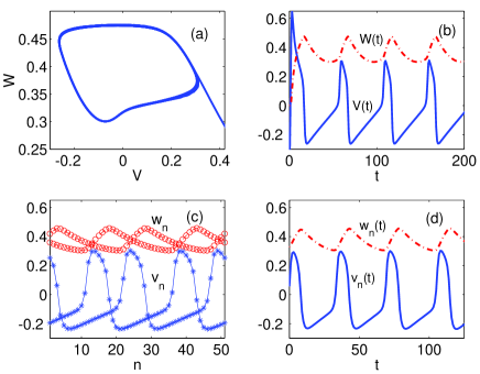
Figure 12: For ML: (a) Limit cycle and (b) Periodic trajectory for an uncoupled unit; (c) spatial profiles at different times: $v_{n}(t)$ (asterisks), $w_{n}(t)$ (circles); (d) temporal profiles of $v_{n}(t)$ (solid line) and $w_{n}(t)$ (dashed line) for $n=20$ fixed. Parameter values are $I=0.375$, $D=0.5$, $\lambda=0.01$.

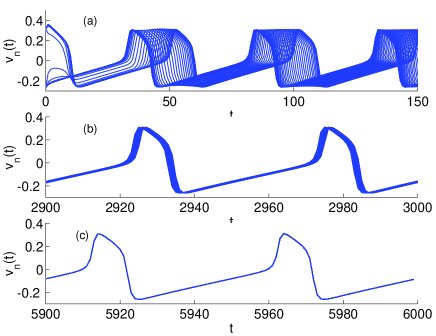
Figure 13: Synchronization in the Morris-Lecar model. We have superimposed the time evolution of $N=50$ oscillators. Parameter values are $I=0.375$, $D=0.5$ and $\lambda=0.01$.

6 Conclusions

We have studied wave propagation and oscillatory behavior in excitable and self-oscillatory one dimensional systems with one fast and one slow variables. In excitable systems, we have constructed asymptotically a one-parameter family of stable wave trains with increasing periods and speeds. Our numerical experiments suggest that the stability of wave trains in discrete systems can be characterized analytically in terms of the dispersion law, as it happens for wave trains in continuous systems [19]. When the spatial period tends to infinity, we obtain the fastest wave of the family: a solitary pulse. As the strength of the coupling between nodes decreases, the family of wave trains becomes smaller. The disappearance of the solitary pulse marks the onset of propagation failure due to spatial discreteness. The critical coupling is the pinning threshold for the leading edge of the pulse in a reduced bistable equation. Close to failure, the wave profiles develop steps and propagation becomes saltatory. Instead of propagating smoothly, the excitation jumps from node to node. Another source of propagation failure is the small separation of time scales for excitation and recovery, shared by continuous models. We obtain bounds for the critical separation of time scales as a function of the coupling. Technically, we have greatly improved the rough bounds contained in [11], derived under very restrictive assumptions on the nonlinearities, which exclude FHN and most realistic sources. Such bounds are unknown in the continuum case. For small $D$, we also develop an asymptotic theory of failure as $\lambda$ decreases. Our asymptotic predictions show a good agreement with numerical solutions of FHN and ML models.

In self-oscillatory systems, wave trains are generated choosing scaled periodic configurations as initial data. For other initial configurations, we observe synchronization phenomena. In the limit of small coupling, we find an equation for the time evolution of the oscillator phases. A detailed analysis of this equation which would support the numerical evidence of synchronization remains to be done.

Acknowledgments. This work has been supported by the Spanish MCyT through grant BFM2002-04127-C02, and by the European Union under grant HPRN-CT-2002-00282. The author thanks Prof. L.L. Bonilla for fruitful discussions.

References

- [1] A.R.A. Anderson and B.D. Sleeman, Wave front propagation and its failure in coupled systems of discrete bistable cells modelled by FitzHugh-Nagumo dynamics, Int. J. Bif. Chaos, 5 (1995) 63-74.
- [2] G.W. Beeler, H.J. Reuter, Reconstruction of the action potential of ventricular mycardial fibers, J. Physiol., 268 (1977) 177-210.
- [3] C.M. Bender, S.A. Orszag, Advanced mathematical methods for scientists and engineers, McGraw-Hill 1978.
- [4] L.L. Bonilla, H.T. Grahn, Non-linear dynamics of semiconductor superlattices, Rep. Prog. Phys., 68 (2005), 577-683.
- [5] V. Booth, T. Erneux, Understanding propagation failure as a slow capture near a limit point, SIAM J. Appl. Math., 55 (1995) 1372-1389.
- [6] J.W. Cahn, Theory of crystal growth and interface motion in crystalline materials, Acta Metall., 8 (1960) 554-562.
- [7] A. Carpio, S.J. Chapman, S. Hastings, J.B. McLeod, Wave solutions for a discrete reaction-diffusion equation, Eur. J. Appl. Math., 11 (2000) 399-412.
- [8] A. Carpio, L.L. Bonilla, Depinning transitions in discrete reaction-diffusion equations, SIAM J. Appl. Math., 63 3 (2003), 1056-1082.
- [9] A. Carpio, L.L. Bonilla, Pulse propagation in discrete systems of coupled excitable cells, SIAM J. Appl. Math., 63 2 (2002) 619-635.
- [10] T. Erneux, G. Nicolis, Propagating waves in discrete reaction-diffusion systems, Phys. D, 67 (1993) 237-244.
- [11] X. Chen, S.P. Hastings, Pulse waves for a semi-discrete Morris-Lecar type model J. Math. Biol., 38 (1999) 1-20.
- [12] G. Fáth, Propagation failure of traveling waves in a discrete bistable medium, Physica D, 116 (1998) 176-180.
- [13] R. FitzHugh, Impulses and physiological states in theoretical models of nerve membrane, Biophys. J., 1 (1961) 445-466; J. Nagumo, S. Arimoto, S. Yoshizawa, An active impulse transmission line simulating nerve axon, Proc. Inst. Radio Engineers, 50 (1962) 2061-2070.
- [14] J. Grasman, Asymptotic methods for relaxation oscillations and applications, Applied Mathematical Sciences 63, Springer New York, 1987.
- [15] J.P. Keener, Propagation and its failure in coupled systems of discrete excitable cells, SIAM J. Appl. Math. 47 (1987) 556-572.
- [16] J.P. Keener, Waves in excitable media, SIAM J. Appl. Math., 39, 528, (1980).
- [17] Y. Kuramoto, T. Tsuzuki, Persistent propagation of concentration waves in dissipative media far from thermal equilibrium, Prog. Theor. Phys., 55 (1976) 356-369.
- [18] P. A. Lagerstrom, Matched asymptotic expansions. Springer, N. Y. 1988.
- [19] K. Maginu, Stability of periodic traveling wave solutions with large spatial periods in reaction-diffusion systems, J. Diff. Eqs, 39 (1981) 73-99.
- [20] K. Maginu, Stability of spatially homogeneous periodic solutions of reaction-diffusion equations, J. Diff. Eqs 31 (1979) 130-138.
- [21] J. Mallet-Paret, The global structure of traveling waves in spatially discrete dynamical systems, J. Dynam. Diff Eqs., 11 (1999), 1-47.
- [22] C. Morris, H. Lecar, Voltage oscillations in the barnacle giant muscle-fiber, Biophys. J., 35 (1981) 193-213.
- [23] J.C. Neu, Chemical waves and the diffusive coupling of limit oscillators, SIAM J. Appl. Math., 36 (1979) 509-515.
- [24] J.C. Neu, Large populations of coupled chemical oscillators, SIAM J. Appl. Math., 38 (1980) 305-316.
- [25] S. Binczak, J.C. Eilbeck, A.C. Scott, Ephaptic coupling of myelinated nerve fibers, Phys. D 148 (2001), 159-174.
- [26] A. Tonnelier, McKean caricature of the FitzHugh-Nagumo model: Traveling pulses in a discrete diffusive medium, Phys. Rev. E, 67 (2003) 036105.
- [27] B. Zinner, Existence of traveling wave front solutions for the discrete Nagumo equation, J. Diff. Eqs., 96 (1992) 1-27.