New perspectives on the Ising model
Abstract
The Ising model, in presence of an external magnetic field, is isomorphic to a model of localized interacting particles satisfying the Fermi statistics. By using this isomorphism, we construct a general solution of the Ising model which holds for any dimensionality of the system. The Hamiltonian of the model is solved in terms of a complete finite set of eigenoperators and eigenvalues. The Green’s function and the correlation functions of the fermionic model are exactly known and are expressed in terms of a finite small number of parameters that have to be self-consistently determined. By using the equation of the motion method, we derive a set of equations which connect different spin correlation functions. The scheme that emerges is that it is possible to describe the Ising model from a unified point of view where all the properties are connected to a small number of local parameters, and where the critical behavior is controlled by the energy scales fixed by the eigenvalues of the Hamiltonian. By using algebra and symmetry considerations, we calculate the self-consistent parameters for the one-dimensional case. All the properties of the system are calculated and obviously agree with the exact results reported in the literature.
I Introduction
It is really very hard to say something new on the Ising model. The model, originally proposed by LenzLenz (1920) in 1920, was exactly solved for the case of an infinite chain by IsingIsing (1925) in 1925. Since then, thousand and thousand of articles and several books have been published on the subject. The reason is that the model is very simple, but still can be considered as the prototype for systems subject to second order phase transitions and can be effectively used for studying critical phenomena. Moreover, the model and its generalizations and modifications can also be used for studying a large variety of physical systems. We do not attempt to summarize the enormous work done in these 80 years; it would go well beyond the purpose of this article. An excellent historical presentation of the Ising model can be found in Ref. Brush, 1967, although it is old and obviously not updated. With no pretension of being exhaustive and complete, we here summarize the principal approaches used in these 80 years.
A basic tool is the transfer matrix methodKramers and Wannier (1941, 1951); Montroll (1941, 1942). By means of this approach, OnsagerOnsager (1944) in 1944 succeed to give an exact solution of the model for a cubic two-dimensional lattice in absence of external magnetic field. The theory of spinors and Lie algebra was used to simplify the Onsager solution Kaufman (1949); Newell and Montroll (1953). Among the exact results for the two-dimensional case, the calculation of the magnetizationYang (1952) and the writing of the spin correlation function in the form of a Toeplitz determinantMontroll et al. (1963) have to be mentioned. Other simplifications of the Onsager solution have been obtained by means of the Jordan-Wigner transformation and fermionization methods Schultz et al. (1964); Lieb et al. (1961); Lieb and Mattis (1962). Different approaches are based on combinatorial methodsKac and Ward (1952); Vdovichenko (1965a, b) and pfaffian methodsHurst and Green (1991); Green and Hurst (1964); Kasteleyn (1963); McCoy and Wu (1973). More recent approaches have seen the Ising Hamiltonian expressed as a Gaussian Grasmannian actionSamuel (1980); Nojima (1998). Along this line, use of operatorial symmetries that simplify the algebra of the transfer matrix has led to the calculation of the partition function for a large class of latticesPlechko (1985, 1988).
Many approximation methods have been used with the goal of obtaining an expression for the partition function valid over a large temperature range: mean field theory, Bethe approximationBethe (1935), cluster variational methodsKikuchi (1951), Monte Carlo simulations, series expansions. The spin correlation functions have been studied at the critical temperatureKadanoff (1969) and in the asymptotic regionWu (1966); Au-Yang (1977). To study critical phenomena and critical indices, tools like series expansions Kirkwood (1938); Domb (1960); Domb and Hunter (1965), scalingPatashinskii and Pokrovskii (1966); Widom (1965); Kadanoff (1966), renormalization group theoryWilson (1971, 1975) have been used.
In spite of the tremendous work done, many problems remain unsolved. The exact partition function in a finite magnetic field is still unknown for dimensions higher than one. Very few exact results have been obtained for the three-dimensional model. There is no exact solution for the two-layer Ising model either. Most of all, a general approach which works in all dimensions and under general boundary conditions, although in some approximation, is needed.
In a recent workMancini (2005), we have shown that there is a large class of models which are exactly solvable in terms of a finite number of parameters that have to be self-consistently calculated. The purpose of the present paper is to apply the method proposed in Ref. Mancini, 2005 to the Ising model and to show that an exact solution of the model does exist for any dimension. In Section 2, we introduce the Ising model for a -dimensional cubic lattice and show that the model is isomorphic to a system of localized spinless interacting particles, satisfying the Fermi statistics. In Section 3, the Hamiltonian of the latter model is solved, that is, a complete finite set of eigenoperators and the relative eigenvalues are determined. Then, as shown in Section 4, the exact form of the retarded Green’s function (GF) and of the correlation function (CF) can be obtained. In Section 5, we derive a set of equations for determining the charge/spin correlation functions. As the composite operators do not satisfy a canonical algebra, the GF, the CF and the charge/spin correlation functions depend on a set of internal parameters not calculable by the dynamics. For the one-dimensional case, by means of the composite operator methodMancini and Avella (2003); Mancini (2003); Mancini and Avella (2004), we calculate these internal parameters (Section 6) and the charge/spin correlation functions (Section 7). Although obvious, it is worth noticing that all the results reproduce the exact solution known in the literature.
What are the advantages of the present method and what is new in the context of the Ising model? We present a new scheme of calculations for treating the model. The scheme is general and can be applied to any dimension. In the framework of this scheme we show that the model is always solvable for all dimensions. The energy spectra of the system are known. In the one dimensional case we show that the energy scales determined by the spectra rule the behavior at the critical temperature. It is reasonable to expect that this is true also for higher dimensions. General relations among different spin correlation functions have been obtained. These are exact relations and might be used to check the consistency of some approximate treatments or numerical calculations. In order to get quantitative results for the cases of two and three dimensions we have to determine a finite small number of parameters. All the properties of the Ising model, the magnetization, the thermodynamical quantities, the spin correlation functions, depend on these parameters that have to be self-consistently determined. By using algebra and symmetry considerations we calculate these parameters for the case . Extension of the calculations to higher dimensions is under investigation.
II The Ising model
The Ising model, in presence of an uniform external magnetic field , is described by the following Hamiltonian
| (1) |
are spin variables, residing on a -dimensional Bravais lattice of sites spanned by the vectors . The variables takes only two values: up or down, or more simply . For a hypercubic lattice of lattice constant with nearest neighbor interactions, the exchange matrix is given by
| (2) |
where is the dimensionality of the system and runs over the vectors in the first Brillouin zone. The exchange constant can be positive or negative, and accordingly the coupling will be ferromagnetic or antiferromagnetic. According to (2), the Hamiltonian (1) can be rewritten as
| (3) |
where
| (4) |
It is worth to recall that the Ising Hamiltonian (1) is invariant under the transformation
| (5) |
Let us consider a system of interacting spinless fermions residing on the same lattice and let and be the related annihilation and creation operators. These operators are Heisenberg fields satisfying canonical anticommutation relations
| (6) |
As a consequence of the algebra (6), each site can be occupied at most by a single particle. The occupation number of the site , , takes only the values 0 and 1. By taking into account two-body interactions, the Hamiltonian for such a system reads as
| (7) |
where is the chemical potential and is the potential. This model Hamiltonian can be connected to the Ising model by defining
| (8) |
It is clear that
| (9) |
By substituting (8) into (7) and by considering only a nearest-neighbor potential we can rewrite the Hamiltonian (7) in the following form
| (10) |
where we defined
| (11) |
Hamiltonian (10) is just the Ising Hamiltonian (3) as we have the equivalence
| (12) |
The relation between the partition functions is
| (13) |
Then, the thermal average of any operator assumes the same value in both models
| (14) |
According to this, we can choose to study either one or the other model and get both solutions at once. We decide to put attention to the model Hamiltonian (7), which for a nearest-neighbor potential reads as
| (15) |
where
| (16) |
III Composite operators and equations of motion
It is immediate to see that the charge density operator satisfies the equation of motion
| (18) |
Then, standard methods based on the use of equations of motion and Green’s function (GF) formalism are not immediately applicable. Indeed, it is easy to check that the causal propagator [ is the chronological operator] and the correlation function assume the form
| (19) |
where is the zero frequency functionMancini and Avella (2003) which cannot be calculated by means of the dynamics111 Use of the formula , where is the causal propagator defined in terms of fermionic algebra Mancini and Avella (2003) would lead just to an identity..
Then, in order to solve the Hamiltonian (15) let us consider the composite operator
| (20) |
This field satisfies the equation of motion
| (21) |
By taking higher-order time derivatives we generate a hierarchy of composite operators. However, we observe that for the number operator satisfies the following algebra
| (22) |
Therefore, the hierarchy of composite operators (20) must close for a certain value of and we should be able to derive a finite closed set of eigenoperators of the Hamiltonian. To this purpose, on the basis of (22) the following fundamental property of the field can be established
| (23) |
where the coefficients satisfy the relation
| (24) |
The proof of Eq. (23) and the explicit expressions of the coefficients are given in Appendix A for the cases . We now define the composite operator
| (25) |
After (23), this field is an eigenoperator of the Hamiltonian (15)
| (26) |
where the matrix , the energy matrix, is defined in Appendix B. It is easy to see that the eigenvalues of the energy matrix are given by
| (27) |
The Hamiltonian (15) has been solved since we know a complete set of eigenoperators and eigenvalues, and we can proceed to the calculations of observable quantities. This will be done in the next Sections by using the Green’s function formalism .
IV Retarded and correlation functions
We define now the thermal retarded Green’s function
| (28) | |||||
where denotes the quantum-statistical average over the grand canonical ensemble. By introducing the Fourier transform
| (29) |
and by means of the Heisenberg equation (26) we obtain the equation
| (30) |
where is the Fourier transform of the normalization matrix, defined as
| (31) | |||||
The solution of Eq. (30) is
| (32) |
The spectral density matrices are calculated by means of the formulaMancini and Avella (2003, 2004)
| (33) |
where is the matrix whose columns are the eigenvectors of the matrix . The explicit expressions of are given in Appendix B. The spectral density matrices satisfy the sum rule
| (34) |
where are the spectral moments defined as
| (35) |
stays for the Fourier transform. It is a consequence of the theorem proved in Ref. Mancini, 1998 [see also pag. 572 in Ref. Mancini and Avella, 2003] that the spectral density matrices, for , satisfy the sum rule (34). The explicit expressions of and are given in Appendices C and D, respectively, for the cases . The correlation function
| (36) |
can be immediately calculated from (32) by using the spectral theorem and one obtains
| (37) |
| (38) |
with
| (39) |
Equations (32) and (38) are an exact solution of the model Hamiltonian (15). One is able to obtain an exact solution as the composite operators constitute a closed set of eigenoperators of the Hamiltonian. However, as stressed in Ref. Mancini and Avella, 2003, the knowledge of the GF is not fully achieved yet. The algebra of the field is not canonical: as a consequence, the normalization matrix in the equation ( 30) contains some unknown static correlation functions, correlators (see Appendix C for explicit calculations), that have to be self-consistently calculated. According to the scheme of calculations proposed by the composite operator method Mancini and Avella (2003); Mancini (2003); Mancini and Avella (2004)(COM), one way of calculating these unknown correlators is by specifying the representation where the GF are realized. The knowledge of the Hamiltonian and of the operatorial algebra is not sufficient to completely determine the GF. The GF refer to a specific representation (i.e., to a specific choice of the Hilbert space) and this information must be supplied to the equations of motion that alone are not sufficient to completely determine the GF. Usually, the use of composite operators leads to an enlargement of the Hilbert space by the inclusion of some unphysical states. Since the GF depend on the unknown correlators, it is clear that the value of these parameters and the representation are intimately related. The procedure is the following. We set up some requirements on the representation and determine the correlators in order that these conditions be satisfied. From the algebra it is possible to derive several relations among the operators. We will call algebra constraints (AC) all possible relations among the operators dictated by the algebra. This set of relations valid at microscopic level must be satisfied also at macroscopic level, when expectations values are considered. Use of these considerations leads to some self-consistent equations which will be used to fix the unknown correlators appearing in the normalization matrix. An immediate set of rules is given by the equation
| (40) |
where the l.h.s. is fixed by the AC and the boundary conditions compatible with the phase under investigation, while in the r.h.s. the correlation function is computed by means of equation of motion [cfr. Eq. (38)].
Another important set of AC can be derived by observing that there exist some operators, , which project out of the Hamiltonian a reduced part
| (41) |
When and commute, the quantum statistical average of the operator O over the complete Hamiltonian must coincide with the average over the reduced Hamiltonian
| (42) |
Another relation is the requirement of time translational invariance which leads to the condition that the spectral moments, defined by Eq. (35 ), must satisfy the following relation
| (43) |
It can be shown that if (43) is violated, then states with a negative norm appear in the Hilbert space. Of course the above rules are not exhaustive and more conditions might be needed.
According to the calculations given in appendices C and D, the GF and the correlation functions depend on the following parameters: external parameters , internal parameters , and , defined as
| (44) |
| (45) |
The parameters are determined by means of their own definitions (44), where the r.h.s. is calculated by means of ( 37)-(38). This equation gives
| (46) |
From the results given in the Appendices C and D, we see that the spectral density matrices have the form
| (47) |
where the matrices and do not depend on momentum . Putting (47) into (46) we obtain
| (48) |
Calculations given in the Appendices C and D show that the matrices are linear combinations of the matrix elements . Then, Eq. (48) gives a system of homogeneous linear equations. The determinant of this system is only function of the external parameters . This function will vanish only if there is a particular relation among these parameters. Since these parameters are independent variables the only solution is that all the matrix elements must vanish
| (49) |
The matrices are zero and the correlation function does not depend on momentum, as we expected. In the coordinate space the CF takes the expression
| (50) |
The correlation function depends on internal parameters: . In order to determine these parameters, we use the Pauli condition (40) which gives the self-consistent equations
| (51) |
where is calculated by means of (50). New correlation functions
| (52) |
appear and the set of self-consistent equations (51) is not sufficient to determine all unknown parameters. One needs more conditions. In the case of one-dimensional systems these extra conditions can be obtained by using the property (42).
V Charge correlations functions
In Sections 3 and 4, we have solved the problem of the Ising model in terms of a set of local parameters, defined by (45) and (52). In this Section, we want to show how we can calculate non-local correlation functions. Let us define the causal Green’s function (for simplicity in this Section we drop the superindex )
| (53) | |||||
the retarded and advanced functions
| (54) | |||||
the correlation functions
| (55) |
where is the composite field defined in (25) and we used the fact the field operator does not depend on time. The Fourier transforms of these quantities read as
| (56) |
where By means of the equation of motion (26) we have
| (57) |
| (58) |
where the matrix is defined as
| (59) |
The most general solution of Eq. (57) is
| (60) | |||||
where
| (61) |
while the function must be determined. denotes the principal value. By recalling the retarded and advanced nature of , it is immediate to see that
| (62) |
Therefore
| (63) |
The solution of (58) is
| (64) |
where the matrices and have to be determined. From the definitions (53)-(55) we can derive the following exact relations
| (65) |
A relation between the two correlation functions and can be established by means of trace properties. Indeed, it is straightforward to derive a KMS-like relation
| (66) | |||||
By recalling the definitions (55), this last equations can be written as
| (67) |
where is the fermionic correlation function [see Eq. ( 37)-(38)]. Therefore, the anticommutator in (65) can be expressed in terms of the correlation functions as
| (68) |
Analogous expression holds for the commutator. By means of (68) and by recalling that [see Eqs. (37)-(38)]
| (69) |
we find that equations (65) have the following form
| (70) |
| (71) |
By recalling that , the solution of (70) and (71,) is:
| (72) | |||||
| (73) | |||||
By putting (72) and (73) into (60) and (64) we have
| (74) | |||||
| (75) | |||||
| (76) | |||||
From the study of the fermionic sector we have
| (77) |
where are the spectral functions given in Appendix D. Then, at equal time (74) becomes
| (78) |
The system (78) gives a system of linear equations for the quantities . Since the inhomogeneous terms in this system are proportional to , it is clear that . Then, we will take and we write
| (79) |
From (78) we have the system of equations
| (80) |
where
| (81) |
From its own definition (79) and by using the recurrence relation ( 23), the matrix has the following structure.
(i) One dimension
| (82) |
| (83) |
(ii) Two dimensions
| (84) |
| (85) |
(iii) Three dimensions
| (86) |
| (87) |
With the definitions
| (88) |
Then, we only need to calculate the matrix elements . The matrix can be obtained from the normalization matrix , calculated in Appendix C, by means of the following substitution
| (89) |
Then, the matrices have the same expressions of the spectral matrices when the following substitution
| (90) |
is made. It can be seen that for and the system (80) is exactly equivalent to the system (51). Then, it is enough to consider the case . In this case, the system (80) becomes
| (91) |
with given by (39). The system (91) gives a set of exact relations among the correlation functions. We might think to solve this system by induction method, since some of the first correlation functions can be expressed in terms of the basic parameters and . However, when we do this, we immediately see that the number of equations is not sufficient to determine all the correlation functions and we need more equations. Once again, this can be done for the one dimensional system, as we shall see in the next Sections.
VI Self-consistent equations for one-dimensional systems
Until now the analysis has been carried on in complete generality for a cubic lattice of dimensions. We now consider one-dimensional systems, and in particular we will study an infinite chain in the homogeneous phase. For simplicity of notation we shall drop the superindex . By means of ( 207) and (222)-(223) the set of equations (51) gives the linear system
| (92) |
where, because of translational invariance, we put
| (93) |
It is immediate to see that for , the solution of the first equation in (92) for is
| (94) |
This is in agreement with the particle-hole symmetry enjoyed by the model [see (17)]. Recalling (8) and (11), this situation corresponds to the zero magnetization of the Ising model in absence of external magnetic field. Coming back to general value of , it is clear that Eqs. (92) are not sufficient to specify completely the 4 parameters and we need another equation. A fourth equation can be easily obtained by means of the algebra. We observe that
| (95) |
This relation leads to
| (96) |
where
| (97) |
By means of the requirement (42) the correlation function can be written as
| (98) |
where
| (99) |
and denotes the thermal average with respect to . Let us define the retarded GF
| (100) | |||||
By means of the equation of motion
| (101) |
we have
| (102) |
Recalling the relation between retarded and correlation functions, from (102) we obtain
| (103) |
By putting this result into (98) we have
| (104) |
By noting that can be expressed as [cfr. (151 )]
| (105) |
we obtain from (104) the relations
| (106) | |||||
| (107) |
Now, we observeFedro (1976) that describes a system where the original lattice is divided in two disconnected sublattices (the chains to the left and to the right of the site ). Then, in -representation, the correlation function which relates sites belonging to different sublattices can be decoupled:
| (108) |
for and belonging to different sublattices. By using this property, invariance of under axis reflection and (106) we can write
| (109) | |||||
By putting (109) into (107), we obtain the following self-consistent equation among the correlation functions
| (110) |
By means of (37) and (38) and the results given in Appendices C and D, Eq. (110) takes the expression
| (111) |
This equation together with equations (92) gives a system of 4 self-consistent equations for the 4 parameters as functions of . By solving the set of linear equations (92) with respect to as functions of , we have
| (112) | |||||
To calculate the parameter let us put (112) into (111) and solve with respect to . We have two roots. One solution corresponds to an unstable state with negative compressibility and must be disregarded. By picking up the right root, and by using the relation
| (115) |
we find
| (116) |
As shown in Appendix E, the solutions (112)-(116) exactly correspond to the well-known solution of the 1D Ising model, obtained by means of the transfer matrix method. We could manipulate the expression (116) and the ones for and , obtained by substituting (116) into (112)-(VI), in order to reproduce the expressions of the Ising model, given in Appendix E. However, we prefer to maintain the present expressions as the following discussion will be more transparent. In Section 3, we have seen that in the present model, in the one-dimensional case, there are three energy scales
| (117) |

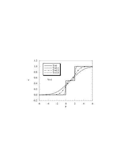
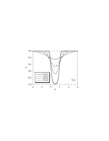
At zero temperature, the three functions , and are not analytical functions at the points and , respectively, and we expect that the parameters exhibit some discontinuous behavior at these points. As shown in Fig. 1, in the limit the particle density has a discontinuity at for the case of negative (i.e. , ferromagnetic coupling) and two discontinuities at and for the case of positive (i.e. , antiferromagnetic coupling). Here and in the following, we take : all energies are measured in units of . In particular, the particle density increases by increasing from zero to one. At zero temperature, in the ferromagnetic case is zero for and equal to one for ; in the antiferromagnetic case is zero for , jumps to and exhibits a plateau, centered at , in the region , jumps to the value for . The parameter has a behavior similar to .
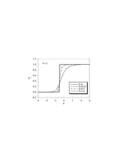
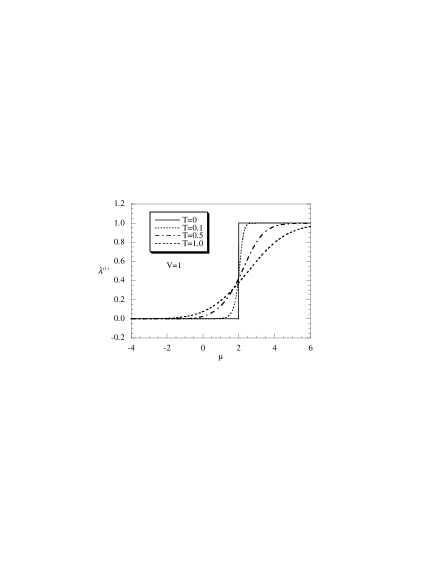
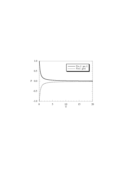
In Fig. 2 we give the parameter as a function of . For the ferromagnetic case the behavior is similar to that of . Instead, in the antiferromagnetic case , at , exhibits only one discontinuity point at , where jumps from zero to one. The parameter has a behavior similar to . The different behavior exhibited by the pairs and for is naturally due to the antiferromagnetic correlations, when we recall that the pair describes a correlation between two first neighboring sites, while describes correlations between two second neighboring sites. Of course in the point of discontinuity the two limits and are not interchangeable. As we shall see in the next Section, the 4 local parameters are really basic since all the properties of the model are described in terms of them. It is worthwhile to note that some simple relations can be established among the parameters
| (118) |
| (119) |
The Ising model in one dimension can be described in terms of only two parameters: and .
VII Charge correlation functions for one-dimensional systems
The system of equations (91) establishes some relations among the non-local charge correlation functions and . As already discussed, the number of equations is not sufficient to determine completely the charge correlation functions, and one needs more equations to close the system. In the one-dimensional case a fourth equation can be easily obtained by algebraic considerations. Recalling that we can easily derive the following result
| (120) |
Now, for (because of invariance under axis reflection we could choose as well), using the property (108)
| (121) | |||||
| (122) |
Therefore, from (120)
| (123) |
| (124) | |||||
| (125) | |||||
where we used Eq. (106). Equations (123) and (124) give
| (126) |
| (127) |
Putting (127) into (125) we get the fourth self-consistent equation
| (128) | |||||
It is straightforward to verify that (128) is identically satisfied for , while for coincides with equation (119).
By adding (128) to (91), we have the following system of equations for the non-local spin correlation functions and
| (129) |
| (130) |
| (131) |
| (132) |
where we put
| (133) |
| (134) |
and we used . To calculate for general we proceed by induction.
Let us put and concentrate the attention on the spin CF . We start by observing that
| (135) |
where the two parameters have been calculated in the fermionic sector. By taking we can calculate from the system (129)-(132) that
| (136) |
The results (135)-(136) and use of the relation (118) show that for can be cast in the form
| (137) |
where the parameter is defined as
| (138) |
By using the expressions of the basic parameters given in Section 5, it is possible to check that . Then, we can introduce the Fourier transform and reexpress (137) as
| (139) |
where
| (140) |
Then, the CF can be calculated as
| (141) | |||||
Therefore, Eq. (137) is valid for any . Recalling the definition of , we can rewrite (137) under the form
| (142) |
Also, from (139) we see that the zero frequency function [cfr. (19)] has the expression
| (143) |
By putting the obtained expression of in Eqs. (129 )-(132), we can solve the system. The solution gives
| (144) |
| (145) | |||||
| (146) |
| (147) |
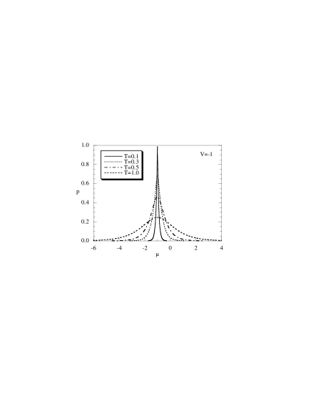
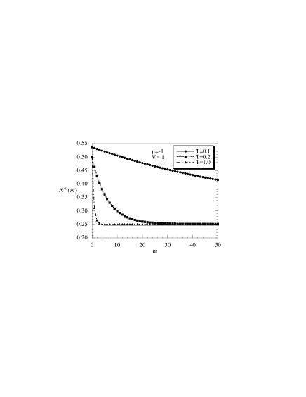
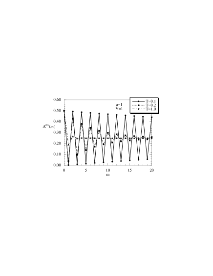
In Fig. 3 we give as a function of for and at various temperatures. We see that for negative (ferromagnetic case), is positive and various between zero and 1. For positive (antiferromagnetic case), is negative and various between and zero. In particular, for negative , tends to 1 at in the limit . Instead, for positive , tends to at in the limit . This is seen in Fig. 4 where is plotted versus at and at .
Let us now discuss the correlation functions. is plotted against for [Fig. 5 (top)] and for [Fig. 5 (bottom)] at various temperatures. We see that when zero temperature is approached a long-range order of ferromagnetic and antiferromagnetic type is established, respectively. Also, we can see from ( 141)-(147) that for and (i.e. not at the critical temperature) the spin correlation functions assume the ergodic value. At the critical temperature we have breakdown of the ergodicity.
VIII Conclusions
The Ising model in presence of an external magnetic field is isomorphic to a model of localized spinless interacting particles, satisfying the Fermi statistics. The latter model belongs to a class of models always solvable, as shown in Ref. Mancini, 2005. On this basis, we have constructed a general solution of the Ising model which holds for any dimensionality of the system. The Hamiltonian of the model has been solved in terms of a complete finite set of eigenoperators and eigenvalues. The Green’s function and the correlation functions of the fermionic model are exactly known and are expressed in terms of a finite small number of parameters that have to be self-consistently determined. By using the equation of the motion method, we have derived a set of equations which connect different spin correlation functions. The scheme that emerges is that it is possible to describe the Ising model from a unified point of view where all the properties are connected to a small number of local parameters, and where the critical behavior is controlled by the energy scales fixed by the eigenvalues of the Hamiltonian. The latter considerations have been proved from a quantitative point of view in the one-dimensional case, where the equations which determine the self-consistent parameters and the spin correlation function have been solved. For all the properties of the system have been calculated and obviously agree with the exact results reported in the literature. Extension of the calculations to higher dimensions is under investigation.
After the paper was completed and submitted for publication, the author learned that approaches to the spin-1/2 Ising model based on a fermionization of the model have been previously reported in Refs. Tyablikov and Fedyanin, 1967 and Kalashnikov and Fradkin, 1969a. The author wishes to thank the referee and Prof. L. De Cesare for putting these papers to his attention. In particular, in Ref. Tyablikov and Fedyanin, 1967, Tyablikov and Fedyanin showed that the chain of equations for the double-time GF closes and the number of equations is determined only by the co-ordination number, independently by the dimensionality. This conclusion agrees with the results given in Sections 3 and 4. In order to close the set of equations for the fermionic correlation functions in the one-dimensional case, the authors of Ref. Tyablikov and Fedyanin, 1967 assumed ergodicity and solved the system, obtaining the exact solution of the 1D Ising model for an infinite chain. It should be remarked that ergodicity breaks down for finite systems and at the critical points. Kalashnikov and Fradkin in Ref. Kalashnikov and Fradkin, 1969a used the spectral density method Kalashnikov and Fradkin (1969b) to derive a system of equations for the correlation functions; also in this case the approach is valid for any dimension. However, the number of equations is less than the number of correlation functions.
Appendix A Algebraic relations
As mentioned in Section 3, the number density operator satisfies the algebra
| (148) |
From this algebra an important relation can be derived. for the operator
| (149) |
where are the first neighbors of the site . We shall discuss separately the cases of different dimensions.
A.1 One dimension
We start from the equation
| (150) |
After subtracting the terms and , we can use the algebraic relation (148) to obtain
| (151) |
with
| (152) |
From (151), by putting we obtain
| (153) |
By substituting (153) into (151) we have the recurrence rule
| (154) |
where
| (155) | |||||
| (156) |
We note that the coefficients satisfy the relation
| (157) |
In table 1 we give the values of the ’s for .
| p | ||
|---|---|---|
| 1 | 1 | 0 |
| 2 | 0 | 1 |
| 3 | ||
| 4 | ||
| 5 | ||
| 6 |
A.2 Two dimensions
We start from the equation
| (162) | ||||
| (165) |
By proceeding as in the case of one dimension, use of the algebraic relation (148) leads to
| (166) |
where the operators are defined as
| (167) |
and the coefficients have the expressions
| (168) |
By solving the system (166) with respect to variables , we can obtain the recurrence rule
| (169) |
where the coefficients are defined as
| (170) |
We note that for all p
| (171) |
In table 2 we give the values of the ’s for
A.3 Three dimensions
We start from the equation
| (176) | ||||
| (179) | ||||
| (184) |
Because of the algebraic relations (148) we obtain
| (185) |
where the operators are defined as
| (186) | ||||
| (187) | ||||
| (188) | ||||
| (189) | ||||
| (190) |
and the new coefficients have the expressions
| (191) |
By solving the system (185) with respect to variables , we can obtain the recursion rule
| (192) |
where the coefficients are defined as
| (193) |
We note that for all p
| (194) |
In table 3 we give the values of the ’s for .
Appendix B The energy matrix
The energy matrix , defined by Eq. (26) can be immediately calculated by means of the equation of motion (21) and the recurrence rule (23) [see Tables 1, 2, 3]. The matrix is defined as the matrix whose columns are the eigenvectors of the matrix . In this Appendix we report the expressions of and for the various dimensions.
B.1 One dimension
| (195) |
B.2 Two dimensions
| (196) |
| (197) |
B.3 Three dimensions
| (198) |
| (199) |
Appendix C The normalization matrix
We recall the definition of the normalization matrix
| (200) | |||||
It is straightforward to see that use of the hermiticity condition (43 ) leads to the fact that we have to calculate only the matrix elements . The calculations of these is very easy when one observes the following anticommutating rule
| (201) |
By taking the expectation value of (201) we obtain in momentum space
| (204) | |||||
with the definitions
| (205) |
C.1 One dimension
| (206) |
where
| (207) |
C.2 Two dimensions
| (208) |
where
| (209) |
C.3 Three dimensions
| (210) |
where
| (211) |
Appendix D The spectral matrices
The spectral density matrices can be immediately calculated by means of the knowledge of the matrices and through Eq. (33).
D.1 One dimension
| (218) | ||||
| (222) |
where
| (223) |
D.2 Two dimensions
| (229) | |||||
| (235) |
| (236) |
| (242) | |||||
| (248) |
with
| (249) |
D.3 Three dimensions
| (254) | |||||
| (259) |
| (264) | |||||
| (269) |
| (270) |
| (275) | |||||
| (280) |
here
| (281) |
The coefficients are given in Table 4.
Appendix E Relations between the Ising and spinless model
In this Appendix, we want to recall the main results of the Ising model and establish the relations between the two models. For an infinite chain the simplest method is the use of the transfer matrix method. The details of calculations are well known and can be found in many textbooks. For example, we refer the reader to Refs.Baxter (1982); Goldenfel (1992); Lavis and Bell (1999). The magnetization per site is given by
| (282) |
The two-point correlation function has the expression
| (283) |
where
| (284) |
and are the eigenvalues of the transfer matrix
| (285) |
The three-point correlation function is given byMarsh (1966)
| (286) |
The relations between the Ising and fermionic models are
| (287) |
| (288) |
| (289) |
| (290) |
| (291) |
By recalling (116) and by means of (288), the magnetization in the fermionic model has the expression
| (292) |
By oserving that and can be expressed as
| (293) |
it is straigtforward to see that (292) is the same as (282). In the fermionic model, by means of (142), we have
| (294) |
where the parameter is expressed in terms of and by means of (138). By using (VI) and (116), and by recalling (115) and (293), it is easy to see that the expression of , given by (138) is exactly equal to the expression (284). Then, the two-point correlation function of the fermionic model exactly agree with the expression (283) of the Ising model. The parameters , and can be calculated in the fermionic model by putting (116) into (112)-( VI), and in the Ising model by means of (289)-(291). After lengthy, but straightforward, calculations, using the relations (115) and (293), it is possible to show that there is an exact agreement.
References
- Lenz (1920) W. Lenz, Z. Physik 21, 613 (1920).
- Ising (1925) E. Ising, Z. Physik 31, 253 (1925).
- Brush (1967) S. G. Brush, Rev. Mod. Phys. 39, 883 (1967).
- Kramers and Wannier (1941) H. A. Kramers and G. H. Wannier, Phys. Rev. 60, 252 (1941).
- Kramers and Wannier (1951) H. A. Kramers and G. H. Wannier, Phys. Rev. 60, 263 (1951).
- Montroll (1941) E. W. Montroll, J. Chem. Phys. 9, 706 (1941).
- Montroll (1942) E. W. Montroll, J. Chem. Phys. 10, 61 (1942).
- Onsager (1944) L. Onsager, Phys. Rev. 65, 117 (1944).
- Kaufman (1949) B. Kaufman, Phys. Rev. 76, 1232 (1949).
- Newell and Montroll (1953) G. F. Newell and E. W. Montroll, Rev. Mod. Phys. 25, 353 (1953).
- Yang (1952) C. N. Yang, Phys. Rev. 85, 808 (1952).
- Montroll et al. (1963) E. W. Montroll, R. B. Potts, and J. C. Ward, J. Math. Phys. 4, 308 (1963).
- Schultz et al. (1964) T. D. Schultz, D. C. Mattis, and E. H. Lieb, Rev. Mod. Phys. 36, 856 (1964).
- Lieb et al. (1961) E. H. Lieb, T. D. Schultz, and D. C. Mattis, Ann. Phys. 16, 407 (1961).
- Lieb and Mattis (1962) E. H. Lieb and D. C. Mattis, Phys. Rev. 125, 164 (1962).
- Kac and Ward (1952) M. Kac and J. C. Ward, Phys. Rev. 88, 1332 (1952).
- Vdovichenko (1965a) N. V. Vdovichenko, Soviet Phys. JETP 20, 470 (1965a).
- Vdovichenko (1965b) N. V. Vdovichenko, Soviet Phys. JETP 21, 350 (1965b).
- Hurst and Green (1991) C. A. Hurst and H. S. Green, J. Chem. Phys. 33, 1059 (1991).
- Green and Hurst (1964) H. S. Green and C. A. Hurst, Order-Disorder Phenomena (Interscience Publishers, New York, 1964).
- Kasteleyn (1963) P. W. Kasteleyn, J. Math. Phys. 4, 287 (1963).
- McCoy and Wu (1973) B. M. McCoy and T. T. Wu, The Two-Dimensional Ising Model (Harvard U.P., Cambridge, Mass., 1973).
- Samuel (1980) S. Samuel, J. Math. Phys. 21, 2806 and 2015 and 2820 (1980).
- Nojima (1998) K. Nojima, Int. J. Mod. Phys. B 12, 1995 (1998).
- Plechko (1985) V. N. Plechko, Theo. Math. Phys. 64, 748 (1985).
- Plechko (1988) V. N. Plechko, Physica A 152, 51 (1988).
- Bethe (1935) H. A. Bethe, Proc. Roy. Soc. A 150, 552 (1935).
- Kikuchi (1951) R. Kikuchi, Phys. Rev. 81, 988 (1951).
- Kadanoff (1969) L. P. Kadanoff, Phys. Rev. 188, 859 (1969).
- Wu (1966) T. T. Wu, Phys. Rev. 149, 380 (1966).
- Au-Yang (1977) H. Au-Yang, Phys. Rev. B 15, 2704 (1977).
- Kirkwood (1938) J. G. Kirkwood, J. Chem. Phys. 6, 70 (1938).
- Domb (1960) C. Domb, Advances in Physics 9, 150 (1960).
- Domb and Hunter (1965) C. Domb and D. L. Hunter, Proc. Roy. Soc. 86, 1147 (1965).
- Patashinskii and Pokrovskii (1966) A. Z. Patashinskii and V. L. Pokrovskii, Soviet Phys. JETP 23, 292 (1966).
- Widom (1965) B. Widom, J. Chem. Phys. 43, 3892 (1965).
- Kadanoff (1966) L. P. Kadanoff, Physics 2, 263 (1966).
- Wilson (1971) K. G. Wilson, Phys. Rev. B 4, 3171 (1971).
- Wilson (1975) K. G. Wilson, Rev. Mod. Phys. 47, 773 (1975).
- Mancini (2005) F. Mancini, Europhys. Lett. 70, 485 (2005).
- Mancini and Avella (2003) F. Mancini and A. Avella, Eur. Phys. J. B 37, 37 (2003).
- Mancini (2003) F. Mancini, in Highlights in Condensed Matter Physics, edited by A. Avella, R. Citro, C. Noce, and M. Salerno (American Institute of Physics, New York, 2003), pp. 240–257.
- Mancini and Avella (2004) F. Mancini and A. Avella, Advances in Physics 53, 537 (2004).
- Mancini (1998) F. Mancini, Physics Letters A 249, 231 (1998).
- Fedro (1976) A. J. Fedro, Phys. Rev. B 14, 2983 (1976).
- Tyablikov and Fedyanin (1967) S. V. Tyablikov and V. K. Fedyanin, Fisika metallov and metallovedenie 23, 193 (1967).
- Kalashnikov and Fradkin (1969a) O. K. Kalashnikov and E. S. Fradkin, Sov. Phys. JETP 28, 976 (1969a).
- Kalashnikov and Fradkin (1969b) O. K. Kalashnikov and E. S. Fradkin, Sov. Phys. JETP 28, 317 (1969b).
- Baxter (1982) R. J. Baxter, Exactly solved models in statistical mechanics (Academic Press, London, 1982).
- Goldenfel (1992) N. Goldenfel, Lectures on phase transitions and the renormalization group (Perseus Pyblishing, Reading, Massachusetts, 1992).
- Lavis and Bell (1999) D. A. Lavis and G. M. Bell, Statistical Mechanics of Lattice Systems, vol. 1 of Text and Monographs in Physics (Springer-Verlag, Berlin, 1999), 2nd ed.
- Marsh (1966) J. S. Marsh, Phys. Rev. 145, 251 (1966).