A Worm Algorithm for Two-Dimensional Spin Glasses

Abstract

A worm algorithm is proposed for the two-dimensional spin glasses. The method is based on a low-temperature expansion of the partition function. The low-temperature configurations of the spin glass on square lattice can be viewed as strings connecting pairs of frustrated plaquettes. The worm algorithm directly manipulates these strings. It is shown that the worm algorithm is as efficient as any other types of cluster or replica-exchange algorithms. The worm algorithm is even more efficient if free boundary conditions are used. We obtain accurate low-temperature specific heat data consistent with a form $c\sim T^{-2}\exp\bigl{(}-2J/(k_{B}T)\bigr{)}$, where $T$ is temperature and $J$ is coupling constant, for the $\pm J$ two-dimensional spin glass.

Spin glasses have been studied for many years from various points of views Edwards . However, the nature of low-temperature phases is still not clarified. Much of the work on spin glasses relies on computer simulations. Monte Carlo simulation has been one of the main tools. The Metropolis algorithm proposed more than half a century ago served well for many of the simulational work, but for spin glasses, it is hampered by extremely long relaxation times at low temperatures. There have been a number of more efficient techniques, noticeably the simulated tempering Marinari and parallel tempering exchange . In two-dimensions (2D), cluster algorithms SW ; replicaMC ; Liang ; Houdayer exist which are quite efficient.

The idea of generating random walks of loops in Monte Carlo simulation has a surprisingly long history earlyloop . The loop algorithms for quantum systems evertz are examples. Recently, several worm algorithms are proposed Prokofev ; Hitchcock for the ferromagnetic Ising and other models. Such algorithms have the advantage that the Monte Carlo updates are purely local, while their effects are global. The classical worm algorithms based on high-temperature expansion variables such as $\tanh(J_{ij}/k_{B}T)$ do not work for spin glasses as the weights would be negative for the antiferromagnetic interactions. In this paper, we propose a worm algorithm for the two-dimensional spin glasses. Our starting point can be thought of as a low-temperature expansion for the partition function. Our algorithm turns out as efficient as the best cluster algorithms Houdayer , replica Monte Carlo replicaMC or replica exchange algorithms exchange . Moreover, large systems can be simulated since we may only simulate one system at a time.

In the following, we outline a base algorithm and then show how to enhance it by multi-step moves. We discuss the efficiency of few variations of the algorithm. We report extensive simulation results for the low-temperature specific heat with periodic and free boundary conditions.

The weight of a spin-glass configuration is proportional to the Boltzmann factor $\exp\bigl{(}\sum_{\langle i\,j\rangle}J_{ij}\sigma_{i}\sigma_{j}/(k_{B}T)\bigr{)}$, where $\sigma_{i}=\pm 1$, and the site $i$ is on an $L\times L$ square lattice with periodic boundary conditions. The summation is over the nearest neighbor pairs. For simplicity, we consider the $\pm J$ spin glass where $J_{ij}=+J$ or $-J$ with equal probability, although the method is not limited to this model. By multiplying the weight by a configuration-independent constant, we can rewrite it in an equivalent form:

$$\prod_{\langle i\,j\rangle}w^{b_{ij}},$$ (1)

where, $w=\exp(-2K)$, $K=J/(k_{B}T)$; the variable $b_{ij}=\frac{1}{2}(1-J_{ij}\sigma_{i}\sigma_{j}/J)$ represents presence (1) or absence (0) of an unsatisfied bond. The bonds live on the dual square lattice. Note that the variables $b_{ij}$ are not independent. They should be set up in such a way that an even number of bonds incident on an unfrustrated plaquette, while an odd number of bonds incident on a frustrated plaquette. A groundstate is one such that all the frustrated plaquettes are paired and connected by strings with minimum total length optimize . At excited states, closed loops of strings can form.

The worm algorithm directly manipulates these strings. The weight, Eq. (1), can be sampled with a “worm” if we extend the phase space to include a path of a worm, with a moving head at location $i$, and a tail at a fixed location $i_{0}$. The weight is exactly the same as before, except that the parity requirement for the head and tail is reversed. That is, a frustrated plaquette at head or tail requires an even number of bonds, and unfrustrated plaquette an odd number of bonds. The movement of the worm must preserve the constraint on the bonds. A valid configuration of the original problem is formed when the worm traces out a closed loop.

The sites and bonds in the following refer to the dual lattice. The base algorithm of the worm movement with a periodic boundary condition is as follows:

1. Pick a site $i_{0}$ at random as the starting point. Set $i\leftarrow i_{0}$.

2. Pick a nearest neighbor $j$ with equal probability, and move it there with probability $w^{1-b_{ij}}$. If it is accepted, flip the bond variable $b_{ij}$ ($0\leftrightarrow 1$) along the way, update $i\leftarrow j$.

3. If $i$ is at the same site as $i_{0}$ and winding numbers are even, one Monte Carlo loop is finished (exit and take statistics), else go to step 2.

We define the winding numbers as the algebraic sum of displacements $\sum\delta{\bf r}$ divided by the linear size $L$ when the head and tail meet. The requirement that the winding numbers must be even is due to the constraints of the bonds on the dual lattice and the spins on the original lattice. A one-to-two mapping to spin configurations is possible and valid from a bond configuration only if the worm winds the system an even number of times in both directions. However, for free boundary conditions, where the spins at the boundary have fewer neighbors, the winding number constraints are not needed. Because both the bond variables and spin variables are available, any desired thermodynamic quantities, such as spin-glass susceptibility, can be obtained. The algorithm is nothing but a Metropolis sampling on the extended phase space. It is ergodic, any state can be reached with nonzero probability, except at zero temperature. We also note that the difference between a ferromagnetic Ising model and a spin glass is only at the initial configuration. In the case of the 2D ferromagnetic Ising model, because of duality, the same bond configuration can also be interpreted as a high-temperature expansion loop configuration at its dual temperature. Thus, the present algorithm is exactly a dual algorithm of Ref. Prokofev for the 2D ferromagnetic Ising model.

The basic algorithm can be systematically enhanced by applying the N-fold way Bortz or “absorbing Markov chain” method Novotny . Note that we are only interested in the configuration when the worm forms a closed path, and do not care about the (Monte Carlo) dynamics while the worm is making its way to meet the tail. We can apply an $n$-step acceleration if it is $n$-step away from the tail $i_{0}$.

Consider a set $A$ of states in state space, consisting of the current state and a collection of neighborhood states of the current state. For example, in our application, we can consider all the states reachable from current state in $n-1$ steps of moves or less. We calculate the escape probability, $P(\nu|\mu)$, of exiting $A$ to state $\nu$ given that it is in state $\mu$. Let $W^{AA}_{\mu\nu}$ be the one-step transition matrix elements of the Markov chain for states within the set $A$ from $\mu$ to $\nu$, and $W^{A\bar{A}}_{\mu\nu}$ for one-step transition probability with $\mu\in A$, but $\nu\in\bar{A}$, where $\bar{A}$ is the complement of $A$. Then the escape probability is given by

$$P(\nu|\mu)=\sum_{k=0}^{\infty}[(W^{AA})^{k}W^{A\bar{A}}]_{\mu\nu}=[(I-W^{AA})^{-1}W^{A\bar{A}}]_{\mu\nu},$$ (2)

where $I$ is an identity matrix. The total escape probability is one, $\sum_{\nu}P(\nu|\mu)=1$. Given the current state $\mu$, the state $\nu\in\bar{A}$ is sampled with the probability $P(\nu|\mu)$. The escape probability can be calculated explicitly. Let the current state be called 0, and its 4 neighbor states by one step move 1 to 4. A new state is uniquely specified by a path of the moves defined by the base algorithm, given the current state. One-step escape probability is $P(0\to\mu)=d_{0}W_{0\mu}$, $\mu=1,2,3,4$. $d_{0}=1/(1-W_{00})$ is fixed by normalization. This is just the original N-fold way of Bortz et al. Bortz . For a two-step move, from the current site 0 to an intermediate site $a$ and reaching $\nu$, the escape probability is $P(0\to a\to\nu)=d_{0}W_{0a}W_{a\nu}/(1-W_{aa})$ where $d_{0}$ is again fixed by normalization. Probabilities for three or more steps are slightly more complicated, but can be worked out. In this work, we consider $n=0$ (no acceleration), and $n=1$ to 4 step accelerations.

At very low temperatures, it can take an exceedingly long time to generate one loop. In this case, it is actually correct to interrupt the simulation by setting a fixed upper limit to the number of steps used for each loop. Those attempts that exceed the upper limit will be treated as rejected moves.

We measure the performance of the algorithm by its correlation times. The correlation times are defined through the correlation functions of the overlapping spin-glass order parameter:

$$f(t)=\left[{\langle Q(t+t^{\prime})Q(t^{\prime})\rangle-\langle Q(t^{\prime})\rangle^{2}\over\langle Q(t^{\prime})^{2}\rangle-\langle Q(t^{\prime})\rangle^{2}}\right]_{J},$$ (3)

where the angular brackets denote average of Monte Carlo loop moves $t^{\prime}$ and the outer square brackets mean average over the quenched random couplings $J_{ij}$. The quantity $Q$ is the overlap of the spins of two independent configurations,

$$Q=\bigl{|}\sum_{i}\sigma_{i}^{1}\sigma_{i}^{2}\bigr{|}.$$ (4)

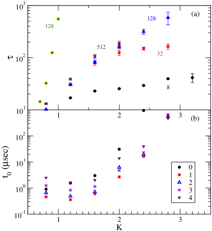
Figure 1: (a) Exponential relaxation times in units of loop trials of the worm algorithm for system sizes $L\times L$ where $L=8$, 32, 128, and 512, vs. dimensionless inverse temperature $K=J/(k_{B}T)$. For comparison, the result of single-spin-flip Metropolis algorithm on $L=128$ is also plotted. (b) CPU time ($\mu$sec) per loop trial per lattice site for a $32\times 32$ lattice on a $2.4\,$GHz AMD Opteron computer, without (0) or with $n$-step acceleration.

Figure 1 demonstrates the efficiency of the algorithm for various sizes and inverse dimensionless temperature $K=J/(k_{B}T)$. The results are from linear fits of the form $\ln f(t)=-t/\tau+c$ in a window $[\tau,3\tau]$. The correlation functions are very close to a pure exponential with $c\approx 0$. The top part, Fig. 1(a), shows correlation time $\tau$ in units of loop moves, the bottom part (b) shows the central processor unit (CPU) times. It is useful to separate the effect of the intrinsic dynamics defined by the base algorithm from the speed-up due to differences in detailed implementation. The correlation time in Fig. 1(a) is independent which of the N-fold-way is used since the N-fold-way preserves the dynamics. They all give the same correlation time in units of number of loops generated. The bottom part Fig. 1(b) gives the actual CPU time, $t_{0}$, in microsecond for one loop generation divided by the number of spins. This number is only slightly dependent on system size $L$. The overall efficiency should be measured by the product of the two. It is interesting to note that as $K$ increases, the correlation time $\tau$ saturates and becomes $K$ independent. Unfortunately, the time it takes for generating one loop increases exponentially. Comparing different versions of N-fold-way acceleration, we found that there is a big improvement going from the base algorithm to one-step N-fold-way. Further increasing the step size does not lead to big improvement until very low temperatures. It is clear that, at $T=0$, one step or two step N-fold-way will not be ergodic, the system can be trapped in a configuration. However, if we allow for sufficiently long-ranged multi-step attempts, we can still make moves even at $T=0$.

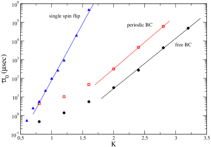
Figure 2: Correlation times, $\tau t_{0}$, measured in actual CPU times for single-spin-flip, 1-step N-fold-way worm algorithm with periodic boundary condition and with a free boundary condition, for $L=128$. The slopes $a$ of the straight line fits to $\exp(aK)$ are 14.0, 6.5, and 6.2, respectively.

What is more remarkable is that a free boundary condition will make the algorithm even more efficient. This is because we can always start from the boundary, or “outside” the system, and the worm will cut the system into pieces. The worm has a much easier job terminating as there are order $L$ more possibilities to hit the boundary comparing to a single site. Conceptually, we can view the system as a planar graph. Various ways of exiting the system can be regarded as moving to the single dual site representing the outside. Fig. 2 gives the correlation times measured in real CPU time, the quantity $\tau t_{0}$. The meaning of this quantity is the amount of CPU time needed in order to decorrelate the system such that the correlation function is reduced to about $e^{-1}$. This is a fair comparison between completely different algorithms, but the results depend on the detail implementation of the computer programs. From this plot, we see that the free boundary condition case is about 20 times more efficient than periodic boundary conditions. The correlation length $\xi$ of the 2D $\pm J$ spin glass diverges as $\exp(2K)$ Kardar ; Houdayer ; Katzgraber . If we define the dynamical critical exponent $z$ as $\tau t_{0}\sim\xi^{z}$, we have $z\approx 7.0$ and 3.2, for the Metropolis single spin flip and the worm algorithms, respectively.

We now turn to the specific heat of the spin glass at low temperatures. In 1988, Wang and Swendsen found by their replica Monte Carlo algorithm that the specific heat of the 2D $\pm J$ spin glass approaches zero according to $c\sim K^{2}\exp(-2K)$ replicaMCPRB . Since the energy gap from the ground states to the first excited states is $4J$, we might expect that the specific heat should go as $\exp(-4K)$. Wang and Swendsen gave an argument in analogous to the 1D Ising model with periodic boundary condition, where although the minimum excitation is also $4J$, the configuration appears in the form of a pair of kinks, each one of them can move freely, so only a single kink with energy $2J$ should be considered “elementary.” Indeed, for 1D Ising model, the specific heat goes as $\exp(-2K)$ in the thermodynamic limit.

However, the above interpretation has been challenged in Ref. Kardar with a method of exact calculation of the partition function and recently in Katzgraber by Monte Carlo simulation, but supported in exact-partition . Thus, the problem is still controversial.

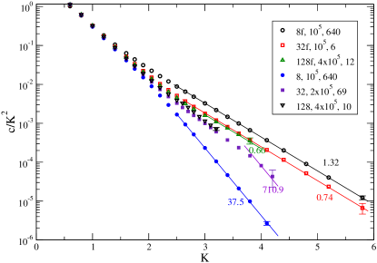
Figure 3: 2D $\pm J$ spin-glass reduced specific heat $c/K^{2}$ vs. $K$. The legend specifies the lattice size $L$ ($f$ for free boundary conditions), Monte Carlo steps, and number of samples of random couplings. The straight lines are fit to $c/K^{2}\approx b\exp(-2K)$ or $b\exp(-4K)$, with $b$ indicated on the lines. The errors at the largest $K$ are mainly due to sample fluctuations.

The present algorithms are well-suited to simulate spin glasses at low temperatures, particularly the free boundary condition version. However, as we can see from Fig. 2, the worm algorithms still have difficulty equilibrating the system when coupling $K>3$. Therefore, we have used a combination of several different algorithms. Each Monte Carlo step consists of several worm loop moves, one sweep of Metropolis single spin flip, replica Monte Carlo between systems at neighboring temperatures and at the same temperature. Three replicas for each temperature are used. With these algorithms, we were able to equilibrate the system down to $K\approx 6$ for $L=8$ and 32, or $K\approx 4$ for $L=128$.

In Fig. 3, we present the reduced specific heat $cK^{-2}$ vs. $K$. The asymptotic slopes for large $K$ should resolve the issue of $2J$ vs. $4J$ controversy. As can be seen from the figure, with periodic boundary conditions, the specific heat eventually settles to $\exp(-4K)$ because of the gap of excitations. However, as $L$ increases, the crossover to a fast decay appears at a larger and larger value of $K$. According to Ref. exact-partition , the cross-over length scale is $l\sim\exp(K)$. This “finite-size-effect” length scale appears different from the correlation length $\xi$, which goes as $\exp(2K)$. On the other hand, the free boundary condition results have a rather different finite-size dependence. We see that the asymptotic form of $\exp(-2K)$ is approached much faster in this case. Of course, since the energy gap with free boundary conditions is $2J$, the final form must be $\exp(-2K)$ for finite sizes. Our data indicate that this is also the form in the thermodynamic limit. Some weak size dependence on the amplitudes is seen, but surprisingly, the thermodynamic limit is obtained much faster with free boundary conditions than with periodic boundary conditions.

In summary, we have shown numerically that the low-temperature specific heat goes like $K^{2}\exp(-2K)$ in the thermodynamic limit. This is observed much clearer with free boundary conditions. Our new calculations support the original argument of Wang and Swendsen regarding the asymptotic form of heat capacity for 2D $\pm J$ spin glass. We demonstrate these results with an efficient worm algorithm. The worm algorithm presented here should be applicable to any models defined on a (planar) graph where the concept of dual graph can be defined. It does not seem possible for 3D lattices. It is also interesting to study the clusters generated in the worm algorithms and to relate them to other quantities. More detailed study will be presented elsewhere.

This work is supported in part by a Faculty Research Grant of National University of Singapore.

References

- (1) K. Binder and A. P. Young, Rev. Mod. Phys. 58, 801 (1986); M. Mézard, G. Parisi, and M. A. Virasoro, Spin Glass Theory and Beyond, Lecture Notes in Physics Vol. 9 (World Scientific, Singapore, 1987); A. P. Young, ed., Spin Glasses and Random Fields, (World Scientific, Singapore, 1998).
- (2) E. Marinari and G. Parisi, Europhys. Lett. 19, 451 (1992).
- (3) K. Hukushima and K. Nemoto, J. Phys. Soc. Jpn 65, 1604 (1996).
- (4) R. H. Swendsen and J.-S. Wang, Phys. Rev. Lett. 58, 86 (1987).
- (5) R. H. Swendsen and J.-S. Wang, Phys. Rev. Lett. 57, 2607 (1986); J.-S. Wang and R. H. Swendsen, Prog. Theor. Phys. Suppl. 157, 317 (2005).
- (6) S. Liang, Phys. Rev. Lett. 69, 2145 (1992).
- (7) J. Houdayer, Eur. Phys. J. B 22, 479 (2001).
- (8) A. Rahman and F. H. Stillinger, J. Chem. Phys. 57, 4009 (1972); A. Yanagawa and J. F. Nagle, Chem. Phys. 43, 329 (1979); G. T. Barkema and M. E. J. Newman, Phys. Rev. E 57, 1155 (1998).
- (9) H. G. Evertz, Adv. Phys. 52, 1 (2003).
- (10) N. Prokof’ev and B. Svistunov, Phys. Rev. Lett. 87, 160601 (2001).
- (11) F. Alet and E. S. Sørensen, Phys. Rev. E 67, 015701(R) (2003); P. Hitchcock, E. S. Sørensen, and F. Alet, Phys. Rev. E 70, 016702 (2004).
- (12) G. Toulouse, Commun. Phys. 2, 115 (1977); F. Barahona, R. Maynard, R. Rammal, and J. P. Uhry, J. Phys. A: Math. Gen. 15, 673 (1982).
- (13) A. B. Bortz, M. H. Kalos, and J. L. Lebowitz, J. Comput. Phys. 17, 10 (1975).
- (14) M. A. Novotny, Phys. Rev. Lett. 74, 1 (1995).
- (15) L. Saul and M. Kardar, Phys. Rev. E 48, R3221 (1993); Nucl. Phys. B 432, 641 (1994).
- (16) H. G. Katzgraber and L. W. Lee, Phys. Rev. B 71, 134404 (2005).
- (17) J.-S. Wang and R. H. Swendsen, Phys. Rev. B 38, 4840 (1988).
- (18) J. Lukic, A. Galluccio, E. Marinari, O. C. Martin, and G. Rinaldi, Phys. Rev. Lett. 92, 117202 (2004).