Superconductivity in C₆Ca explained.

Abstract

Using density functional theory we demonstrate that superconductivity in C₆Ca is due to a phonon-mediated mechanism with electron-phonon coupling $\lambda=0.83$ and phonon-frequency logarithmic-average $\langle\omega\rangle=24.7$ meV. The calculated isotope exponents are $\alpha({\rm Ca})=0.24$ and $\alpha({\rm C})=0.26$. Superconductivity is mostly due C vibrations perpendicular and Ca vibrations parallel to the graphite layers. Since the electron-phonon couplings of these modes are activated by the presence of an intercalant Fermi surface, the occurrence of superconductivity in graphite intercalated compounds requires a non complete ionization of the intercalant.

Graphite intercalated compounds (GICs) were first synthesized in 1861 Schaffautl but only from the 30s a systematic study of these systems began. Nowadays a large number of reagents can be intercalated in graphite ($\gg 100$)DresselhausRev . Intercalation allows to change continuously the properties of the pristine graphite system, as it is the case for the electrical conductivity. The low conductivity of graphite can be enhanced to obtain even larger conductivities than Copper Foley . Moreover at low temperatures, intercalation can stabilize a superconducting stateDresselhausRev . The discovery of superconductivity in other intercalated structures like MgB₂Nagamatsu and in other forms of doped Carbon (diamond) Ekimov has renewed interest in the field.

The first discovered GIC superconductors were alkali-intercalated compoundsHannay (C₈A with A= K, Rb, Cs with T${}_{c}<$ 1 K). Synthesis under pressure has been used to obtain metastable GICs with larger concentration of alkali metals (C₆K, C₃K, C₄Na, C₂Na) where the highest T_c corresponds to the largest metal concentration, T_c(C₂Na)=5 K Belash . Intercalation involving several stages have also been shown to be superconductingAlexander ; Outti (the highest T_c = 2.7 K in this class belongs to KTl_1.5C₄). Intercalation with rare-earths has been tried, C₆Eu, C₆Cm and C₆Tm are not superconductors, while recently it has been shown that C₆Yb has a T_c = 6.5 K Weller . Most surprising superconductivity on a non-bulk sample of C₆Ca was also discoveredWeller . The report was confirmed by measurements on bulk C₆Ca poly-crystalsGenevieve and a $T_{c}=11.5$ K was clearly identified. At the moment C₆Yb and C₆Ca are the GICs with the highest T_c. It is worthwhile to remember that elemental Yb and Ca are not superconductors.

Many open questions remain concerning the origin of superconductivity in GICs. (i) All the aforementioned intercalants act as donors respect to graphite but there is no clear trend between the number of carriers transferred to the Graphene layers and T_cDresselhausRev . What determines T_c? (ii) Is superconductivity due to the electron-phonon interaction Mazin or to electron correlation Csanyi ? (iii) In the case of a phonon mediated pairing which are the relevant phonon modes Mazin ? (iv) How does the presence of electronic donor states (or interlayer states) affect superconductivity DresselhausRev ; Csanyi ; Mazin ?

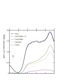
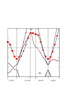
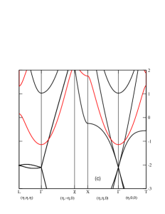
Figure 1: (Color online) (a) Total DOS and DOS projected on selected atomic wavefunctions in C₆Ca. (b) Band structure of C₆Ca. The size of the dots represents the percentage of Ca component. As a reference the dot at $\approx 0.6$ eV at the L-point represents 0.95 Ca component. (c) Band structure of ^∗Ca (Red) and C${}_{6}^{*}$ (black). The bands have been shifted to compare with the C₆Ca band structure. The directions are given in terms of the rombohedral reciprocal lattice vectors. $\chi$ is the interception between the $(\eta,-\eta,0)$ line with the border of the first Brillouin zone ($\eta=0.3581$). The points L, $\Gamma$, X, T have $\eta=0.5$.

Two different theoretical explanations has been proposed for superconductivity in C₆Ca. In Csanyi it was noted that in most superconducting GICs an interlayer state is present at E_f and a non-conventional excitonic pairing mechanismAllender has been proposed. On the contrary Mazin Mazin suggested an ordinary electron-phonon pairing mechanism involving mainly the Ca modes with a 0.4 isotope exponent for Ca and 0.1 or less for C. However this conclusion is not based on calculations of the phonon dispersion and of the electron-phonon coupling in C₆Ca. Unfortunately isotope measurements supporting or discarding these two thesis are not yet available.

In this work we identify unambiguously the mechanism responsible for superconductivity in C₆Ca. Moreover we calculate the phonon dispersion and the electron-phonon coupling. We predict the values of the isotope effect exponent $\alpha$ for both species.

We first show that the doping of a graphene layer and an electron-phonon mechanism cannot explain the observed T_c in superconducting GICs. We assume that doping acts as a rigid shift of the graphene Fermi level. Since the Fermi surface is composed by $\pi$ electrons, which are antisymmetric respect to the graphene layer, the out-of-plane phonons do not contribute to the electron-phonon coupling $\lambda$. At weak doping $\lambda$ due to in-plane phonons can be computed using the results of ref. Piscanec . The band dispersion can be linearized close to the K point of the hexagonal structure, and the density of state per two-atom graphene unit-cell is $N(0)=\beta^{-1}\sqrt{8\pi\sqrt{3}}\sqrt{\Delta}$ with $\beta=14.1$ eV and $\Delta$ is the number of electron donated per unit cell (doping). Only the E_2g modes near $\Gamma$ and the A${}^{\prime}_{1}$ mode near K contribute:

$$\lambda=N(0)\left[\frac{2\langle g^{2}_{\bf\Gamma}\rangle_{F}}{\hbar\omega_{\bf\Gamma}}+\frac{1}{4}\frac{2\langle g^{2}_{\bf K}\rangle_{F}}{\hbar\omega_{\bf K}}\right]=0.34\sqrt{\Delta}$$ (1)

where the notation is that of ref. Piscanec . Using this equation and typical values of $\Delta$ Pietronero the predicted T_c are order of magnitudes smaller than those observed. As a consequence superconductivity in C₆Ca and in GICs cannot be simply interpreted as doping of a graphene layer, but it is necessary to consider the GIC’s full structure.

The atomic structureGenevieve of CaC₆ involves a stacked arrangement of graphene sheets (stacking AAA) with Ca atoms occupying interlayer sites above the centers of the hexagons (stacking $\alpha\beta\gamma$). The crystallographic structure is R3̄m Genevieve where the Ca atoms occupy the 1a Wyckoff position (0,0,0) and the C atoms the 6g positions (x,-x,1/2) with x$=1/6$. The rombohedral elementary unit cell has 7 atoms, lattice parameter 5.17 ${\rm\AA}$ and rombohedral angle $49.55^{o}$. The lattice formed by Ca atoms in C₆Ca can be seen as a deformation of that of bulk Ca metal. Indeed the fcc lattice of the pure Ca can be described as a rombohedral lattice with lattice parameter 3.95 ${\rm\AA}$ and angle $60^{o}$. Note that the C₆Ca crystal structure is not equivalent to that reported in Weller which has a stacking $\alpha\beta$. In Weller the structure determination was probably affected by the non-bulk character of the samples.

Density Functional Theory (DFT) calculations are performed using the PWSCF/espresso codePWSCF and the generalized gradient approximation (GGA) PBE . We use ultrasoft pseudopotentialsVanderbilt with valence configurations 3s²3p⁶4s² for Ca and 2s²2p² for C. The electronic wavefunctions and the charge density are expanded using a 30 and a 300 Ryd cutoff. The dynamical matrices and the electron-phonon coupling are calculated using Density Functional Perturbation Theory in the linear responsePWSCF . For the electronic integration in the phonon calculation we use a $N_{k}=6\times 6\times 6$ uniform k-point meshfootnotemesh and and Hermite-Gaussian smearing of 0.1 Ryd. For the calculation of the electron-phonon coupling and of the electronic density of states (DOS) we use a finer $N_{k}=20\times 20\times 20$ mesh. For the $\lambda$ average over the phonon momentum q we use a $N_{q}=4^{3}$ ${\bf q}-$points mesh. The phonon dispersion is obtained by Fourier interpolation of the dynamical matrices computed on the $N_{q}$ points mesh.

The DFT band structure is shown in figure 1(b). Note that the $\Gamma\chi$X direction and the L$\Gamma$ direction are parallel and perpendicular to the graphene layers. The K special point of the graphite lattice is refolded at $\Gamma$ in this structure. For comparison we plot in 1(c) the band structure of C₆Ca and with Ca atoms removed (C₆^∗) and the structure C₆Ca with C₆ atoms removed (^∗Ca). The size of the red dots in fig. 1(b) represents the percentage of Ca component in a given band (Löwdin population). The ^∗Ca band has a free electron like dispersion as in fcc Ca. From the magnitude of the Ca component and from the comparison between fig. 1(b) and (c) we conclude that the C₆Ca bands can be interpreted as a superposition of the ^∗Ca and of the C₆^∗ bands. At the Fermi level, one band originates from the free electron like ^∗Ca band and disperses in all the directions. The other bands correspond to the $\pi$ bands in C₆^∗ and are weakly dispersive in the direction perpendicular to the graphene layers. The Ca band has been incorrectly interpreted as an interlayer-band Csanyi not associated to metal orbitals.

More insight on the electronic states at E_f can be obtained calculating the electronic DOS. The total DOS, fig. 1(a), is in agreement with the one of ref. Mazin and at E_f it is $N(0)=1.50$ states/(eV unit cell). We also report in fig. 1(a) the atomic-projected density of state using the Löwdin populations, $\rho_{\eta}(\epsilon)=\frac{1}{N_{k}}\sum_{{\bf k}n}|\langle\phi^{L}_{\eta}|\psi_{{\bf k}n}\rangle|^{2}\delta(\epsilon_{{\bf k}n}-\epsilon)$. In this expression $|\phi^{L}_{\eta}\rangle=\sum_{\eta\prime}[{\bf S}^{-1/2}]_{\eta,\eta^{\prime}}|\phi^{a}_{\eta^{\prime}}\rangle$ are the orthonormalized Löwdin orbitals, $|\phi^{a}_{\eta^{\prime}}\rangle$ are the atomic wavefunctions and $S_{\eta,\eta^{\prime}}=\langle\phi^{a}_{\eta}|\phi^{a}_{\eta^{\prime}}\rangle$. The Kohn and Sham energy bands and wavefunctions are $\epsilon_{{\bf k}n}$ and $|\psi_{{\bf k}n}\rangle$. This definition leads to projected DOS which are unambiguously determined and are independent of the method used for the electronic structure calculation. At E_f the Ca 4s, Ca 3d, Ca 4p, C 2s, C 2p_σ and C 2p_π are 0.124, 0.368, 0.086, 0.019, 0.003, 0.860 states/(cell eV), respectively. Most of C DOS at E_f comes from C 2p_π orbitals. Since the sum of all the projected DOSs is almost identical to the total DOS, the electronic states at E_f are very well described by a superposition of atomic orbitals. Thus the occurrence of a non-atomic interlayer-state, proposed in ref. Csanyi , is further excluded. From the integral of the projected DOSs we obtain a charge transfer of 0.32 electrons (per unit cell) to the Graphite layers ($\Delta=0.11$).

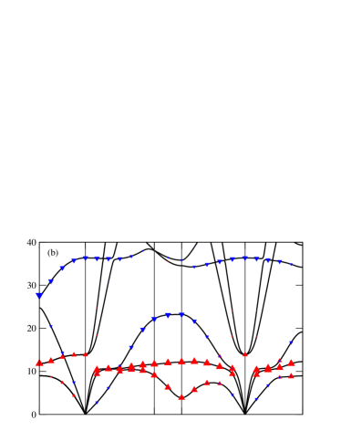
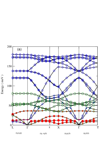
Figure 2: (Color online) (a) and (b) CaC₆ Phonon dispersion. The amount of Ca vibration is indicated by the size of the •, of C_z by the size of $\circ$, of C${xy}$ by the size of $\diamond$, of Ca_xy by the size of $\blacktriangle$ and of Ca_z by the size of $\blacktriangledown$.

The phonon dispersion ($\omega_{{\bf q}\nu}$) is shown in fig. 2. For a given mode $\nu$ and at a given momentum ${\bf q}$, the radii of the symbols in fig.2 indicate the square modulus of the displacement decomposed in Ca and C in-plane ($xy$, parallel to the graphene layer) and out-of-plane ($z$, perpendicular to the graphene layer) contributions. The corresponding phonon density of states (PHDOS) are shown in fig. 3 (b) and (c). The decomposed PHDOS are well separated in energy. The graphite modes are weakly dispersing in the out-of-plane direction while the Ca modes are three dimensional. However the Ca_xy and the Ca_z vibration are well separated contrary to what expected for a perfect fcc-lattice. One Ca_xy vibration is an Einstein mode being weakly dispersive in all directions.

The superconducting properties of C₆Ca can be understood calculating the electron-phonon interaction for a phonon mode $\nu$ with momentum ${\bf q}$:

$$\lambda_{{\bf q}\nu}=\frac{4}{\omega_{{\bf q}\nu}N(0)N_{k}}\sum_{{\bf k},n,m}|g_{{\bf k}n,{\bf k+q}m}^{\nu}|^{2}\delta(\epsilon_{{\bf k}n})\delta(\epsilon_{{\bf k+q}m})$$ (2)

where the sum is over the Brillouin Zone. The matrix element is $g_{{\bf k}n,{\bf k+q}m}^{\nu}=\langle{\bf k}n|\delta V/\delta u_{{\bf q}\nu}|{\bf k+q}m\rangle/\sqrt{2\omega_{{\bf q}\nu}}$, where $u_{{\bf q}\nu}$ is the amplitude of the displacement of the phonon and $V$ is the Kohn-Sham potential. The electron-phonon coupling is $\lambda=\sum_{{\bf q}\nu}\lambda_{{\bf q}\nu}/N_{q}=0.83$. We show in fig.3 (a) the Eliashberg function

$$\alpha^{2}F(\omega)=\frac{1}{2N_{q}}\sum_{{\bf q}\nu}\lambda_{{\bf q}\nu}\omega_{{\bf q}\nu}\delta(\omega-\omega_{{\bf q}\nu})$$ (3)

and the integral $\lambda(\omega)=2\int_{-\infty}^{\omega}d\omega^{\prime}\alpha^{2}F(\omega^{\prime})/\omega^{\prime}$. Three main contributions to $\lambda$ can be identified associated to Ca_xy, C_z and C_xy vibrations.

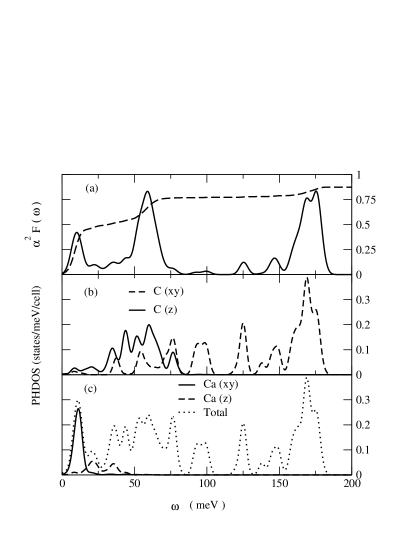
Figure 3: (a) Eliashberg function, $\alpha^{2}F(\omega)$, (continuous line) and integrated coupling, $\lambda(\omega)$ (dashed). (b) and (c) PHDOS projected on selected vibrations and total PHDOS.

A more precise estimate of the different contributions can be obtained noting that

$$\lambda=\frac{1}{N_{q}}\sum_{\bf q}\sum_{i\alpha j\beta}[{\bf G}_{\bf q}]_{i\alpha,j\beta}[{\bf C_{q}}^{-1}]_{j\beta,i\alpha}$$ (4)

where $i,\alpha$ indexes indicate the displacement in the Cartesian direction $\alpha$ of the $i^{\rm th}$ atom, $[{\bf G_{q}}]_{i\alpha,j\beta}=\sum_{{\bf k},n,m}4{\tilde{g}}_{i\alpha}^{*}{\tilde{g}}_{j\beta}\delta(\epsilon_{{\bf k}n})\delta(\epsilon_{{\bf k+q}m})/[N(0)N_{k}]$, and ${\tilde{g}}_{i\alpha}=\langle{\bf k}n|\delta V/\delta x_{{\bf q}i\alpha}|{\bf k+q}m\rangle/\sqrt{2}$. The ${\bf C_{q}}$ matrix is the Fourier transform of the force constant matrix (the derivative of the forces respect to the atomic displacements). We decompose $\lambda$ restricting the summation over $i,\alpha$ and that over $i,\beta$ on two sets of atoms and Cartesian directions. The sets are C_xy, C_z, Ca_xy, and Ca_z. The resulting $\bm{\lambda}$ matrix is:

$$\bm{\lambda}\,=\begin{matrix}&\begin{matrix}{\rm C}_{xy}&{\rm C}_{z}&{\rm Ca}_{xy}&{\rm Ca}_{z}\\ \end{matrix}\\ \begin{matrix}{\rm C}_{xy}\\ {\rm C}_{z}\\ {\rm Ca}_{xy}\\ {\rm Ca}_{z}\\ \end{matrix}&\begin{pmatrix}0.12&0.00&0.00&0.00\\ 0.00&0.33&0.04&0.01\\ 0.00&0.04&0.27&0.00\\ 0.00&0.01&0.00&0.06\\ \end{pmatrix}\end{matrix}$$ (5)

The off-diagonal elements are negligible. The Ca out-of-plane and C in-plane contributions are small. For the in-plane C displacements, eq. 1 with $\Delta=0.11$ gives $\lambda_{{\rm C}_{xy},{\rm C}_{xy}}=0.11$. Such a good agreement is probably fortuitous given the oversimplified assumptions of the model. The main contributions to $\lambda$ come from Ca in-plane and C out-of-plane displacements. As we noted previously the C out-of-plane vibration do not couple with the C $\pi$ Fermi surfaces. Thus the coupling to the C out-of-plane displacements comes from electrons belonging to the Ca Fermi surface. Contrary to what expected in an fcc lattice, the Ca_xy phonon frequencies are smaller than the Ca_z ones. This can be explained from the much larger $\lambda$ of the Ca in-plane modes.

The critical superconducting temperature is estimated using the McMillan formulamcmillan :

$$T_{c}=\frac{\langle\omega\rangle}{1.2}\exp\left(-\frac{1.04(1+\lambda)}{\lambda-\mu^{*}(1+0.62\lambda)}\right)$$ (6)

where $\mu^{*}$ is the screened Coulomb pseudopotential and $\langle\omega\rangle=24.7$ meV is the phonon frequencies logarithmic average. We obtain T${}_{c}=11$K, with $\mu^{*}=0.14$. We calculate the isotope effect by neglecting the dependence of $\mu^{*}$ on $\omega$. We calculate the parameter $\alpha({\rm X})=-\frac{d\log{T_{c}}}{dM_{\rm X}}$ where X is C or Ca. We get $\alpha({\rm Ca})=0.24$ and $\alpha({\rm C})=0.26$. Our computed $\alpha({\rm Ca})$ is substantially smaller than the estimate given in ref. Mazin . This is due to the fact that only $\approx 40\%$ of $\lambda$ comes from the coupling to Ca phonon modes and not $85\%$ as stated in ref.Mazin .

In this work we have shown that superconductivity in C₆Ca is due to an electron-phonon mechanism. The carriers are mostly electrons in the Ca Fermi surface coupled with Ca in-plane and C out-of-plane phonons. Coupling to both modes is important, as can be easily inferred from the calculated isotope exponents $\alpha({\rm Ca})=0.24$ and $\alpha({\rm C})=0.26$. Our results suggest a general mechanism for the occurrence of superconductivity in GICs. In order to stabilize a superconducting state it is necessary to have an intercalant Fermi surface since the simple doping of the $\pi$ bands in graphite does not lead to a sizeable electron-phonon coupling. This condition occurs if the intercalant band is partially occupied, i. e. when the intercalant is not fully ionized. The role played in superconducting GICs by the intercalant Fermi surface has been previously suggested by Jishi . More recently a correlation between the presence of a band, not belonging to graphite, and superconductivity has been observed in Csanyi . However the attribution of this band to an interlayer state not derived from intercalant atomic orbitals is incorrect.

We acknowledge illuminating discussions with M. Lazzeri,G. Loupias, M. d’Astuto, C. Herold and A. Gauzzi. Calculations were performed at the IDRIS supercomputing center (project 051202).

References

- (1) P. Schaffäutl, J. Prakt. Chem. 21, 155 (1861)
- (2) M. S. Dresselhaus and G. Dresselhaus, Adv. in Phys. 51 1, 2002
- (3) G. M. T. Foley, C. Zeller, E. R. Falardeau and F. L. Vogel, Solid. St. Comm. 24, 371 (1977)
- (4) J. Nagamatsu et al., Nature (London), 410, 63 (2001).
- (5) E. A. Ekimov et al. Nature (London), 428, 542 (2004)
- (6) N. B. Hannay, T. H. Geballe, B. T. Matthias, K. Andres, P. Schmidt and D. MacNair, Phys. Rev. Lett. 14, 225 (1965)
- (7) I. T. Belash, O. V. Zharikov and A. V. Palnichenko, Synth. Met. 34, 47 (1989) and Synth. Met. 34, 455 (1989).
- (8) M. G. Alexander, D. P. Goshorn, D. Guerard P. Lagrange, M. El Makrini, and D. G. Onn, Synt. Meth. 2, 203 (1980)
- (9) B. Outti, P. Lagrange, C. R. Acad. Sci. Paris 313 série II, 1135 (1991).
- (10) T. E. Weller, M. Ellerby, S. S. Saxena, R. P. Smith and N. T. Skipper, cond-mat/0503570
- (11) N. Emry et al., cond-mat/0506093
- (12) I. I. Mazin, cond-mat/0504127, I. I. Mazin and S. L. Molodtsov, cond-mat/050365
- (13) G. Csányi et al., cond-mat/0503569
- (14) D. Allender, J. Bray and J. Bardeen, PRB 7, 1020 (1973)
- (15) S. Piscanec et al., Phys. Rev. Lett. 93, 185503 (2004)
- (16) L. Pietronero and S. Strässler, Phys. Rev. Lett. 47, 593 (1981)
- (17) http://www.pwscf.org, S. Baroni, et al., Rev. Mod. Phys. 73, 515-562 (2001)
- (18) J.P.Perdew, K.Burke, M.Ernzerhof, Phys. Rev. Lett. 77, 3865 (1996)
- (19) D. Vanderbilt, PRB 41, 7892 (1990)
- (20) This mesh was generated respect to the reciprocal lattice vectors of a real space unit cell formed by the 120o hexagonal vectors in the graphite plane and a third vector connecting the centers of the two nearby hexagons on neighboring graphite layers. In terms of the real space rombohedral lattice vectors (,,) the new vectors are , , .
- (21) McMillan, Phys. Rev. 167, 331 (1968).
- (22) R. A. Jishi, M. S. Dresselhaus, PRB 45, 12465 (1992)