Speckle-visibility spectroscopy: A tool to study time-varying dynamics

Abstract

We describe a multispeckle dynamic light scattering technique capable of resolving the motion of scattering sites in cases that this motion changes systematically with time. The method is based on the visibility of the speckle pattern formed by the scattered light as detected by a single exposure of a digital camera. Whereas previous multispeckle methods rely on correlations between images, here the connection with scattering site dynamics is made more simply in terms of the variance of intensity among the pixels of the camera for the specified exposure duration. The essence is that the speckle pattern is more visible, i.e. the variance of detected intensity levels is greater, when the dynamics of the scattering site motion is slow compared to the exposure time of the camera. The theory for analyzing the moments of the spatial intensity distribution in terms of the electric field autocorrelation is presented. It is demonstrated for two well-understood samples, a colloidal suspension of Brownian particles and a coarsening foam, where the dynamics can be treated as stationary. However, the method is particularly appropriate for samples in which the dynamics vary with time, either slowly or rapidly, limited only by the exposure time fidelity of the camera. Potential applications range from soft-glassy materials, to granular avalanches, to flowmetry of living tissue.

I Introduction

Dynamic light scattering (DLS) is a powerful tool for probing motion within samples of physical, chemical, biological, and medical interest Cummins and Pike (1974); Berne and Pecora (2000); Chu (1991); Brown (1993); Shepherd and Oberg (1990); Aizu and Asakura (1991); Briers (2001). The physical basis is that the frequency spectrum of the scattered light is Doppler broadened according to the velocities of all the scattering sites. The shape of the spectrum reveals the nature of the motion, for example whether it is ballistic or diffusive; the characteristic width of the spectrum reveals the rate of the motion, for example the root-mean-squared speed or the diffusion coefficient. If the sample is nearly transparent, so that incident photons scatter at most once, then the spectrum can be resolved vs scattering angle in order to probe collective motion at different length scales. This is the single-scattering regime. By contrast if the sample is opaque, so that incident photons scatter off many sites before exiting the sample, then any wavevector-dependence is lost. The art of DLS in this regime is known as diffusing-wave spectroscopy Maret and Wolf (1987); Pine et al. (1988); Weitz and Pine (1993); Maret (1997).

The most straightforward approach to DLS is to measure the frequency spectrum directly, for example using a Fabry-Perot interferometer with a very narrow band pass. However, it is also common practice to deduce the spectrum by an interference technique, in which the scattered light is collected over an area comparable to one speckle spot (spatial-coherence length). The motion of the scattering sites causes corresponding changes in the speckle pattern, and hence large fluctuations in the detected intensity. These fluctuations are quantified by the temporal intensity autocorrelation function, which is simply related to the frequency spectrum under certain conditions (below). This is known as intensity- or photon-correlation spectroscopy (PCS). One advantage of PCS is that digital correlators are commercially available that can compute the intensity autocorrelation over many decades in delay time, for example 10 ns to 100 s. One disadvantage of this approach is that the temporal fidelity is limited by the necessity of sampling over many correlation times to build up statistical weight. This makes them a poor choice for studying systems with dynamics changing on time scales of seconds or faster. Interferometers are useful for large frequency shifts, but do not sport an equally impressive dynamic range. Given the breadth of applications of DLS, it is perhaps not surprising that the essential equivalence of information available from interferometric and correlation-based approaches to DLS is not universally recognized Briers (1996).

In order to ensure simple connection between the intensity autocorrelation and the frequency spectrum of the scattered light, several conditions must be met: (a) There must be many, uncorrelated scattering sites or regions; (b) the extent of the motion must be sufficiently great as to fully randomize the speckle pattern; and (c) the scattering site dynamics must not vary over the time scale of the measurement. The first criterion holds if the sample and scattering volume are sufficiently large; this does not represent a fundamental restriction. The second criterion holds if the sample is fluid or if the scattering sites are bound only loosely to a fixed average location. The third criterion holds if the sample is in thermal equilibrium, or if the sample is in a stationary state in which both the external energy input and the microscopic dynamical response do not fluctuate. Thus, the conditions (a-c) for conventional single-detector PCS to apply are not overly restrictive. It is possible to verify whether not these conditions hold through measurement of higher-order temporal intensity correlations Lemieux and Durian (1999), which can be processed from the raw intensity vs time data stream simultaneously with the second-order intensity autocorrelation.

There are many systems where some of the above conditions do not hold and conventional single-detector PCS does not apply. The kinetics of phase separation, gelation, and aggregation are examples of long-standing interest, in which the dynamics progressively change with time Poon (1998). These processes can be treated as stationary only if the evolution is slow compared to the time scale over which the intensity autocorrelation decays. The broad class of soft-glassy materials comprise another example where the dynamics change with time Cipelletti and Ramos (2005). Furthermore, just as for the gelation problem, the scattering sites can become more tightly bound with age, so that after a certain point the speckle pattern no longer fully randomizes. And lastly, dynamics in granular materials usually cannot be studied with traditional PCS, for example because the input of energy is vibratory or because the response is intermittent avalanche-like flows Jaeger et al. (1996).

Multispeckle dynamic light scattering techniques have been introduced as a useful remedy in such situations where traditional single-detector PCS methods do not apply Wong and Wiltzius (1993); Kirsch et al. (1996). The approach is to compute the temporal autocorrelation function for each pixel of a digital camera, and then to average together the results. Since there are many pixels, and hence many speckles, it is no longer a requirement that motion within the sample cause the speckle pattern to fully randomize. And since the large number of pixels can significantly reduce the time needed to acquire good signal-to-noise, it is easier to study evolving dynamics. However it still remains a challenge to implement multispeckle DLS. A prohibitive difficulty is that commercial multispeckle devices do not exist. A limiting difficulty is either that vast quantities of data must be stored for post-processing or that real-time processing must be made sufficiently fast. Further difficulties arise from the use of charge coupled devices as light sensing elements. Hardware and software advances continue to be reported in the technical literature Cipelletti and Weitz (1999); Lumma et al. (2000); Viasnoff et al. (2002); Xu et al. (2002); Cipelletti et al. (2003); Seydel et al. (2003); Pham et al. (2004); Falus et al. (2004).

In this paper we supply full details and demonstration of a multispeckle dynamic light scattering technique we dub speckle-variance spectroscopy Dixon and Durian (2001) or speckle-visibility spectroscopy (SVS) Dixon and Durian (2003). Our approach is to characterize motion within a sample in terms of the visibility of the speckle pattern formed with scattered light for a single exposure of a digital CCD or CMOS camera. We begin by introducing appropriate notation and the experimental apparatus in the context of the more usual multispeckle DLS. Then we describe the theoretical underpinnings of SVS, and give examples for common types of scattering site dynamics. Our theory contradicts a widely-cited prediction obtained in the context of laser-speckle photography Fercher and Briers (1981). Next, crucially, we demonstrate the validity of our theory by experiments on well-known samples. Finally we discuss experimental considerations for successful implementation of dynamic light scattering with a digital camera.

II Photon-Correlation Spectroscopies

We begin with prerequisite theoretical and experimental background materials necessary for the next sections on SVS.

II.1 Theory

In all DLS experiments, light from a coherent source enters a sample. Some portion scatters, with individual photons experiencing different trajectories, and some fraction of the scattered light reaches a photodetector. Ignoring constant factors, the detector reports a signal proportional to the light intensity, $I(t)=E(t)E^{*}(t)$, where the electric field $E(t)$ is a superposition of many fields representing many photon trajectories. The acquired intensity can be an analog signal, or it can be a bit-stream with each pulse representing a different detected photon. Ultimately, the quantity of interest is either the power spectrum $|E(\omega)|^{2}$ or its Fourier transform: the temporal electric field autocorrelation function. We denote the absolute normalized temporal electric field autocorrelation as

$$g_{1}(\tau)\equiv|\langle E(t)E^{*}(t+\tau)\rangle|/\langle E(t)E^{*}(t)\rangle,$$ (1)

where $\tau$ is the delay time. In traditional PCS the average $\langle\cdots\rangle$ is taken over a range of times $t_{\rm start}<t<t_{\rm stop}$. By definition, $g_{1}(\tau)$ decays from one to zero as $\tau$ ranges from zero to infinity. The characteristic time scale for the decay is the reciprocal of the characteristic width of the power spectrum. If the power spectrum is symmetric and centered around $\omega_{\circ}$, then the normalized (but not absolute) electric field autocorrelation function is $g_{1}(\tau)e^{i\omega_{\circ}\tau}$. For example, a Lorentzian power spectrum $|E(\omega)|^{2}\propto 1/[Dq^{2}+(\omega-\omega_{\circ})^{2}]$ and an exponential field autocorrelation function $g_{1}(\tau)=\exp(-Dq^{2}\tau)$ correspond to light of incident frequency $\omega_{\circ}$ scattered by wavevector $q$ from diffusing particles; the diffusion coefficient $D$ could be extracted from measurement of either the power spectrum or the field autocorrelation.

In single-detector PCS the electric field autocorrelation function is deduced from measurement of the normalized intensity autocorrelation function,

$$g_{2}(\tau)\equiv\langle I(t)I(t+\tau)\rangle/\langle I\rangle^{2}.$$ (2)

This is straightforward only if the three conditions discussed in the Introduction are all met. If (a) the electric field is the superposition of many independent scattered fields and if (b) the field autocorrelation decays to zero over a time scale much shorter than the duration of the measurement, then the Central Limit Theorem implies that $E(t)$ is a Gaussian-distributed complex variable with zero mean. Intuitively, the total field $E(t)=\sum E_{i}(t)$ at some instant of time, $t$, may be evaluated graphically by phasor addition. If there are enough independent scattering regions, then each term in the sum constitutes one step in a random walk in the complex plane. Many such random walks will be sampled, and hence the distribution of values of $E(t)$ over the course of the measurement will be Gaussian, if $g_{1}(\tau)$ fully decays to zero over a shorter time scale than the measurement duration. If the field distribution is Gaussian, then temporal correlations of the form $\langle E(t)E^{*}(t)E(t+\tau_{1})E^{*}(t+\tau_{1})E(t+\tau_{2})E^{*}(t+\tau_{2})\cdots\rangle$ can be expressed as a sum of products of field autocorrelations. For example, the normalized intensity autocorrelation is a four-order field correlation that reduces to

$$g_{2}(\tau)=1+\beta[g_{1}(\tau)]^{2},$$ (3)

where $\beta\leq 1$ is a number determined by the ratio of detector size to speckle spot size. This is widely known as the Siegert relation. A detailed derivation of the Siegert relation, the value of $\beta$, and analogous results for third- and fourth-order temporal intensity correlations, are given in Ref. Lemieux and Durian (1999). To briefly summarize, the method of PCS is to measure $g_{2}(\tau)$ and to extract $g_{1}(\tau)$ using Eq. (3). Subsequent connection is then to be made between $g_{1}(\tau)$ and scattering site dynamics, depending on details of the illumination and detection geometry and on the optical properties of the sample.

In multispeckle PCS methods the intensity autocorrelation is measured at each pixel of a digital camera and the results are averaged together Wong and Wiltzius (1993); Kirsch et al. (1996); Cipelletti and Weitz (1999); Lumma et al. (2000); Viasnoff et al. (2002); Xu et al. (2002); Cipelletti et al. (2003); Seydel et al. (2003); Falus et al. (2004). By virtue of the large number of pixels, the combined statistics of all the detected fields is now Gaussian even if the field autocorrelation never decays to zero. In effect, statistics are sampled by an ensemble average over many speckles rather than by a time-average for a single speckle. Thus the Siegert relation, Eq. (3), may be invoked even more generally for multispeckle PCS than for single-detector PCS.

As an aside, the violation of the Siegert relation in single-detector PCS due to non-randomization of the detected electric field is sometimes said to be due to non-ergodicity of the sample. This is a misnomer and can lead to confusion. The ergodicity of dynamics within the sample, and the ergodicity of the field statistics for the detected light, are distinct issues that may or not be related.

II.2 Experiment

We now apply the above multispeckle PCS technique to a suspension of diffusing Brownian particles. This serves as a starting point from which to demonstrate SVS, since all measurement and sample hardware carry over without change.

The sample consists of 653 nm diameter polystyrene spheres [Duke Scientific] suspended in water at a volume fraction of ten percent. It is poured into a glass beaker, diameter 6 cm, to a depth of 2.4 cm, then sealed. Light from a Coherent Verdi V5 NdYVO₄ Laser, wavelength $\lambda=532$ nm, is expanded and directed almost normal to the bottom of the sample beaker with a Gaussian spot size of $a=1.25$ cm. The outpower of the laser is held fixed, and the illumination intensity is reduced as needed by use of neutral density filters. See the schematic diagram in Fig. 1. According to Mie scattering theory for dilute independent spheres van de Hulst (1957), the scattering length specifying the exponential attenuation of a beam is $l_{s}=24~{}\mu$m, and the average cosine of the scattering angle is $g=0.90$. Therefore, about ten scattering events are required to randomize the photon propagation direction, and the transport mean free path is $l^{*}=l_{s}/(1-g)\approx 240~{}\mu$m. Thus our sample has an opaque white appearance, and we operate in the multiple scattering regime known as diffusing-wave spectroscopy.

In order to perform multispeckle DWS, a portion of the backscattered light leaving the bottom of the sample is reflected by mirror into a Basler-160 digital line scan CCD camera. This device has 1024 pixels, each $10~{}\mu$m $\times$ $10~{}\mu$m and 8 bits deep, and can capture images at a maximum rate of 58 kHz. Except for the mirror and a 532 nm line filter, there are no other optics. The sample-to-camera distance is adjusted to about $d=30$ cm. This gives a speckle size of $s\approx d\lambda/a=13~{}\mu$m, and a ratio of pixel to speckle areas of $A_{\rm pixel}/A_{\rm speckle}\approx 0.6$. The camera is interfaced to a PC equipped with a National Instruments PCI-1422 card, and is programmed using LabVIEW.

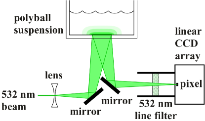
Figure 1: Experimental apparatus for performing both multispeckle dynamic light scattering and speckle-visibility spectroscopy on an opaque colloidal suspension. The orientation of the array of pixels is horizontal, perpendicular to the plane of the drawing.

As a benchmark reference to compare with our SVS technique, our operating procedure is to record the intensity levels in all 1024 pixels for a total of 2 s in increments of $20~{}\mu$s; the entire data set thus consists of 102.4 million 8-bit values. The laser intensity is adjusted so that the average gray-scale value is 40. When the laser is blocked, the signal drops to a “dark count” grayscale value of 3.5. The first step in the analysis is to subtract the dark count and divide by the average remaining signal, thus giving the normalized intensity time trace $I(t)/\langle I\rangle$ for each pixel. A portion of such a trace for one pixel is displayed in Fig. 2. As the colloidal particles diffuse, the intensity level at a pixel indeed fluctuate strongly; here, it is seen to vary between about 0.4 and 4 times the average.

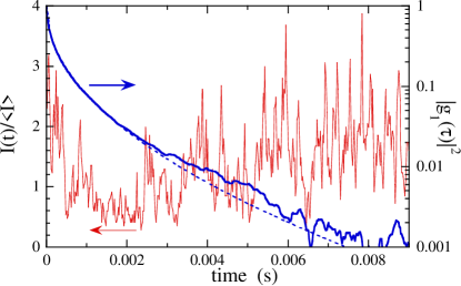
Figure 2: An example of intensity vs time in one pixel (left) and the normalized intensity autocorrelation function $|g_{1}(\tau)|^{2}=[\langle I(0)I(\tau)\rangle/\langle I\rangle^{2}-1]/\beta$ (right), for light backscattered from an opaque colloidal suspension. The intensity autocorrelation is directly computed from the full time-trace, which consists of $10^{5}$ points in 20 $\mu$s time increments for each of the 1024 pixels in the linescan CCD camera. The normalization factor $\beta=0.34$ was obtained by extrapolating the unnormalized intensity autocorrelation to zero delay time. The suspension consists of 653 nm diameter polystyrene spheres in water, at a volume fraction of 10 percent. The theory of diffusing-wave spectroscopy predicts $g_{1}(\tau)\sim\exp[-\gamma\sqrt{6t/t_{o}}]$ where $t_{o}=1/Dk^{2}=6.1$ ms. The fit to this form (dashed curve) gives $\gamma=1.3$.

The observed intensity fluctuations in Fig. 2 display structures lasting over a range of time scales. As is done in multispeckle PCS, this behavior may be quantified by the normalized intensity autocorrelation, $g_{2}(\tau)$ defined by Eq. (2), which we compute directly for each pixel and then average together. According to the Siegert relation, Eq. (3), the zero-time intercept is $g_{2}(0)=1+\beta$. Extrapolating $g_{2}(\tau)$ data to $\tau=0$ gives $\beta=0.34$, which is consistent with the ratio of pixel to speckle areas. Invoking the Siegert relation, we deduce the normalized field autocorrelation $|g_{1}(\tau)|$, and plot its square in Fig. 2. Finding the value of $\beta$ is often referred to as the issue of normalization. Note that the square of $g_{1}(\tau)$ is simply the intensity autocorrelation displayed dimensionlessly on a scale ranging from 1 to 0. Thus, the time scales of structure in the intensity time trace can be compared directly with features in the decay of $|g_{1}(\tau)|^{2}$. Indeed the decay is very fast initially, reflecting the fast fluctuations in $I(t)$. The later-time decay is slower, reflecting the longer-lived fluctuations evident in Fig. 2 as drift in a local average of the intensity.

The above measurement of $g_{1}(\tau)$ may be compared with the predictions of DWS. In the backscattering geometry, with equivalent plane-wave in / plane-wave out illumination and detection, the theory of DWS Weitz and Pine (1993) predicts $g_{1}(\tau)\approx\exp(-\gamma\sqrt{6\tau/\tau_{\circ}})$ where typically $1.5<\gamma<2.5$ and where $\tau_{\circ}\equiv 1/(Dk^{2})$ is the characteristic time for a particle to diffuse a distance $1/k=\lambda/(2\pi n)$ where n is the index of refraction. For our sample, the predicted decay time is $\tau_{\circ}=6.1$ ms. The stretched-exponential form of $g_{1}(\tau)$ reflects the broad length distribution of possible photon paths that contribute to the signal. It also reflects a subtle breakdown of diffusion and continuum approximations for short path lengths Middleton and Fisher (1991); Durian (1995). The value of $\gamma$, but not the stretched-exponential form, is particularly sensitive to the treatment of short paths and can thus be affected by the polarization states, boundary reflectivities, and propagation directions for the incoming and outgoing photons MacKintosh et al. (1989); Vera et al. (1997); Lemieux et al. (1998). Taking the value $\gamma=1.28$, somewhat lower than expectation, we obtain an excellent fit to the data as shown by the dashed curve in Fig. 2. Thus we pronounce our sample, apparatus, dataset, and multispeckle analysis methods as sound. For demonstration of SVS in a later section, the value of $\gamma$ will not be important; we only need a sample with known $g_{1}(\tau)$.

III Speckle-visibility spectroscopy

In this section we develop the theory of speckle-visibility spectroscopy (SVS). The underlying principle of SVS is illustrated in Fig. 3, which displays intensity vs pixel number for four different exposure times, $T$, of the camera. The shortest exposure in Fig. 3, $T=2\times 10^{-5}$ s, is shorter than the decay time of $g_{1}(\tau)$; therefore, the speckle appears static and large intensity differences are registered from pixel to pixel. For longer and longer exposures, the visibility of this speckle pattern progressively fades. This is because the intensity at each individual pixel fluctuates during the exposure and is averaged over the exposure time. In the limit of a very long exposure time in comparison to the decay time, each pixel approaches the same mean intensity value and there is no variation among the pixels. Indeed, the longest exposure in Fig. 3, $T=2\times 10^{-2}$ s, is longer than the decay time of $g_{1}(\tau)$; here, many speckles are sampled at each pixel over the duration of the exposure, and each pixel registers a value close to the average. The very essence of SVS is, thus, to quantify the visibility of the speckle pattern in terms of moments of the distribution of intensities registered by all the pixels for a given exposure duration, and to relate this to the absolute normalized electric field autocorrelation function $g_{1}(\tau)$. A subsequent connection with scattering site dynamics can then be made as per usual DLS practice in either single- or multiple scattering limits.

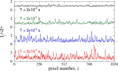
Figure 3: Intensity vs pixel number, ie the profile of the speckle pattern in the plane of the CCD camera, for the same colloidal suspension and optical configuration as in Figure 1. The exposure durations $T$ differ by successive factors of ten, as labelled. Since the speckles change with time, as shown in Fig. 2, their visibility is smaller for longer exposures. This is the essence of SVS.

Before carrying out the theoretical aspects of this program, we note that our method is not without precedent. Perhaps the first is a calculation Jakeman and Pike (1968) and experimental verification Jakeman et al. (1968) of the distribution for the photocurrent as measured by one detector as a function of integration time. Another precedent is “laser-speckle photography” Fercher and Briers (1981), in which the blurring of speckle in a laser-illuminated scene is taken as a signature of motion Aizu and Asakura (1991); Briers (2001). The latter is now being applied to cerebral blood flow, in particular Dunn et al. (2001); Durduran et al. (2004); Weber et al. (2004); Yuan et al. (2005). One aspect of our contribution here is to simplify and generalize the work of Refs. Jakeman and Pike (1968), and to correct a mistake in the widely-cited work of Ref. Fercher and Briers (1981).

III.1 Variance

The variance of intensity across the pixels is a simple way to quantify the visibility of the speckle pattern formed at the imaging array. For a given exposure, each pixel reports a signal that is proportional to the total number of photons it receives. Thus the signal at pixel $i$ is proportional to the time-average of the intensity trace $I_{i}(t)$:

$$S_{i,T}=\int_{0}^{T}I_{i}(t^{\prime}){\rm d}t^{\prime}/T,$$ (4)

where $t=0$ defines the beginning of the exposure and $T$ is the duration of the exposure. The data returned by the camera, for a single exposure, consists of the set $\{S_{i,T}\}$ where the index $i$ ranges from 1 to the total number $N$ of pixels. All quantities of interest are to be computed from the $N$ members of this set. For example the $n^{th}$-moment of the distribution of pixel signals is

$$\langle I^{n}\rangle_{T}=\sum_{i=1}^{N}(S_{i,T})^{n}/N,$$ (5)

where the subscript $T$ is a reminder that the result depends on the exposure duration. Note that these moments represent an ensemble average over pixels for a fixed time interval.

To compute the variance we focus on the first two moments of the signal distribution. The first moment is simply the average intensity, $\langle I\rangle=\sum_{i=1}^{N}S_{i,T}/N$, which is independent of the exposure duration. The second moment is the average over pixels of the quantity

$$(S_{i,T})^{2}=\int_{0}^{T}\int_{0}^{T}I_{i}(t^{\prime})I_{i}(t^{\prime\prime}){\rm d}t^{\prime}{\rm d}t^{\prime\prime}/T^{2}.$$ (6)

Since this is an ensemble average, the Siegert relation Eq. (3) may be invoked: $\langle I_{i}(t^{\prime})I_{i}(t^{\prime\prime})\rangle=\langle I\rangle^{2}\{1+\beta[g_{1}(t^{\prime}-t^{\prime\prime})]^{2}\}$, giving an intermediate result for the second moment as

$$\langle I^{2}\rangle_{T}=\langle I\rangle^{2}\int_{0}^{T}\int_{0}^{T}\{1+\beta[g_{1}(t^{\prime}-t^{\prime\prime})]^{2}\}{\rm d}t^{\prime}{\rm d}t^{\prime\prime}/T^{2}.$$ (7)

The first term in the integral is one; the second term can be reduced to a single integral by recognizing that $g_{1}(t)$ is usually an even function. We now define a normalized variance, and finish the calculation:

$$V_{2}(T) \equiv {1\over\beta}\left[\langle I^{2}\rangle_{T}/\langle I\rangle^{2}-1\right],$$ (8)

$$= \int_{0}^{T}\int_{0}^{T}[g_{1}(t^{\prime}-t^{\prime\prime})]^{2}{\rm d}t^{\prime}{\rm d}t^{\prime\prime}/T^{2},$$ (9)

$$= \int_{0}^{T}2(1-t/T)[g_{1}(t)]^{2}{\rm d}t/T.$$ (10)

This is the fundamental equation of SVS. The top line is a definition; it quantifies speckle visibility on a scale of $0-1$ in terms of the first two moments of the distribution of pixel signal data, $\{S_{i,T}\}$, returned for a given exposure of duration $T$. The middle line is an intermediate step that holds even if $g_{1}(t)$ is not even. The bottom line is where contact usually is to be made between measurement and the underlying normalized electric field autocorrelation. Evidently the variance is a weighted-average of $[g_{1}(t)]^{2}$ over the exposure interval $0<t<T$, with heavier weighting for shorter $t$. This weighting reflects the distribution of possible time differences within an exposure.

III.2 Higher-Order Moments

The distribution of pixel signals is typically skewed toward higher values, as seen for example in Fig. 3; therefore, it is not Gaussian and cannot be fully specified by just the value of the variance. Hence we repeat the calculation leading to the fundamental equation of SVS, Eq. (10), but now for higher-order moments. The results can be useful for diagnosing problems with the experimental apparatus, for deducing the normalization constant $\beta$, and for better testing trial forms of $g_{1}(t)$ for unknown samples.

We define reduced moments of the pixel signal distribution as

$$v_{n}(T)\equiv\langle I^{n}\rangle_{T}/\langle I\rangle^{n}-1.$$ (11)

These are larger for shorter exposures, and vanish for long exposures in the limit that the speckle is no longer visible. While dimensionless, these moments are not normalized in the sense that their values depend on the number of speckles per pixel through $\beta$. Hence we use a lower-case “$v_{n}(T)$” for reduced moments defined in Eq. (11), to contrast with the upper-case “$V_{2}(T)$” for the normalized second moment defined in Eq. (10). Now the task is to compute an ensemble average over pixels $i$ for quantities of form

$$\left\langle\int_{0}^{T}{{\rm d}t_{1}\over T}\int_{0}^{T}{{\rm d}t_{2}\over T}\cdots\int_{0}^{T}{{\rm d}t_{n}\over T}I_{i}(t_{1})I_{i}(t_{2})\cdots I_{i}(t_{n})\right\rangle_{i}.$$ (12)

Invoking third and fourth order Siegert relations Lemieux and Durian (1999), and assuming that $g_{1}(t)$ is even, we arrive at

$$v_{2}(T) = 2\beta\int_{0}^{T}{{\rm d}t\over T}\left(1-t/T\right)[g_{1}(t)]^{2},$$ (13)

$$v_{3}(T) = 3v_{2}(T)+12\beta^{2}\int_{0}^{T}{{\rm d}t_{1}\over T}\int_{t_{1}}^{T}{{\rm d}t_{2}\over T}\left(1-t_{2}/T\right)g_{1}(t_{1})g_{1}(t_{2})g_{1}(t_{2}-t_{1}),$$ (14)

$$v_{4}(T) = 6v_{2}(T)+O(\beta^{2})$$ (15)

The reduced second moment is recognized as $v_{2}(T)=\beta V_{2}(T)$. The third and fourth reduced moments, by contrast, contain terms that are not proportional to $\beta$; therefore, their dependence on the number of speckles per pixel cannot be normalized away by a simple division.

Note that for very short exposure times, the reduced moments approach

$$v_{n}(0)=[1+\beta][1+2\beta]\cdots[1+(n-1)\beta]-1,$$ (16)

which is a well-known result describing the moments of static speckle patterns Lemieux and Durian (1999); Goodman (1984). For long exposure times, the reduced moments vanish as

$$v_{2}(T) \rightarrow 2\beta\int_{0}^{\infty}[g_{1}(t)]^{2}{\rm d}t/T,$$ (17)

$$v_{3}(T) \rightarrow 3v_{2}(T),$$ (18)

$$v_{4}(T) \rightarrow 6v_{2}(T).$$ (19)

No matter what the form of $g_{1}(t)$, the final decay of the moments goes as $v_{n}(T)\sim 1/T$. This is a consequence of the heavy weighting of $g_{1}(t)$ near $t=0$.

III.3 Examples and Precedents

Here we consider the intensity moments predicted by the above formalism for several forms of $g_{1}(\tau)$ of experimental interest. Normalized variance predictions for five special cases are collected in Table 1. The first three of these cases are plotted vs exposure time in Fig. 4. Note that the decay of $V_{2}(T)$ vs $T$ is slower than that of $g_{1}(\tau)$ vs $\tau$; furthermore, the long-time decay is always $V_{2}(T)\sim 1/T$, as explained by Eq. (19). This feature allows the characteristic time scale for the decay of $g_{1}(\tau)$, which is equivalent to the characteristic broadening of the power spectrum, to be extracted even when it is a decade or more faster than the bandwidth of the camera.

$g_{1}(x=\Gamma\tau)$	$V_{2}(x=\Gamma T)$
$\exp(-x)$	$[e^{-2x}-1+2x]/(2x^{2})$
$\exp(-\sqrt{x})$	$[(3+6\sqrt{x}+4x)e^{-2\sqrt{x}}-3+2x]/(2x^{2})$
$\exp(-x^{2})$	$[e^{-2x^{2}}-1+\sqrt{2\pi}x{\rm erf}(\sqrt{2}x)]/(2x^{2})$
$\sqrt{6x}/\sinh{\sqrt{6x}}$	$\zeta(3)/x\approx 1.202/x$, $x\gg 1$
$\sqrt{6x^{2}}/\sinh{\sqrt{6x^{2}}}$	$\sqrt{\pi^{4}/54}/x\approx 1.343/x$, $x\gg 1$

Table 1: Normalized variance predictions, computed from Eq. (10), for various forms of the normalized electric field autocorrelation function, $g_{1}(\tau)$. The first example, $g_{1}(\tau)=\exp(-\Gamma\tau)$, corresponds to single-scattering from sites with diffusive dynamics and to DWS in backscattering for a sample with ballistic dynamics. The second example, $g_{1}(\tau)=\exp(-\sqrt{\Gamma\tau})$, corresponds to DWS in backscattering for a sample with diffusive dynamics. The third example, $g_{1}(\tau)=\exp[-(\Gamma\tau)^{2}]$, corresponds to single-scattering for a sample with ballistic dynamics. These three cases are plotted vs exposure time in Fig. 4. The fourth and fifth examples correspond to DWS in transmission for samples with diffuse and ballistic dynamics, respectively. These forms are too intractable to compute for general exposure times.

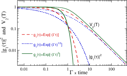
Figure 4: Comparison of $[g_{1}(\tau)]^{2}$ and $V_{2}(T)$, for three types of scattering site dynamics, as labelled. According to prediction, Eq. (10), the latter is a weighted average of the former.

The only case for which we have analytically computed both second and third moments of the pixel signal distribution is for a Lorentzian spectrum or, equivalently, for an exponential field autocorrelation $g_{1}(\tau)=\exp(-\Gamma\tau)$. This corresponds to single-scattering from a sample with diffusive dynamics and to DWS in backscattering from a sample with random ballistic dynamics. For the former, the linewidth or decay rate is $\Gamma=Dq^{2}$ where $D$ is the diffusion coefficient and $q$ is the magnitude of the scattering vector; for the latter, the decay rate is $\Gamma\approx 4\pi\delta v/\lambda$ where $\delta v$ is the root-mean squared average random speed and $\lambda$ is the wavelength of light in the medium. For this example, the reduced second and third moments are

$$v_{2}(T) = \beta{e^{-2x}-1+2x\over 2x^{2}},$$ (20)

$$v_{3}(T) = 3v_{2}(T)+6\beta^{2}{(1+x)e^{-2x}-1+x\over 2x^{3}},$$ (21)

where $x=\Gamma T$ is the product of decay rate and exposure time, as per the notation in Table 1.

The normalized variance for the special case of a Lorentzian spectrum, given in Eq. (21), appeared nearly thirty years ago as Eq. (50) of Ref. Jakeman and Pike (1968). It was subsequently tested experimentally in Ref. Jakeman et al. (1968). This supports our theory of SVS, which seems both simpler and more general than that of Ref. Jakeman and Pike (1968). Our approach applies for any form of $g_{1}(\tau)$, not just for a Lorentzian spectrum, and it also accounts for any number of speckles per pixel. To our knowledge, Eqs. (15a-c) have not previously appeared in the literature.

The special case of a Lorentzian spectrum was also considered in Ref. Fercher and Briers (1981), which is widely cited as a founding paper in the field of laser-speckle flowmetry. There the visibility of a speckle pattern is quantified by “speckle contrast”:

$$K(T)\equiv\sigma_{T}/\langle I\rangle,$$ (22)

where $\sigma_{T}$ is the standard deviation of the set of intensities as measured over an exposure of duration $T$. This quantity equals the square root of our reduced variance, $K(T)=\sqrt{v_{2}(T)}$. The quoted result for a Lorentzian spectrum, Eq. (9) of Ref. Fercher and Briers (1981) and Eq. (13) of a more recent review Briers (2001), would give $v_{2}(T)$ as the following unweighted average of $[g_{1}(\tau)]^{2}$ over the exposure interval:

$$\int_{0}^{T}[g_{1}(t)]^{2}{\rm d}t/T={1-e^{-2x}\over 2x},$$ (23)

where $x=\Gamma T$ as before. This conflicts with Eq. (21) here, and with Eq. (50) of Ref. Jakeman and Pike (1968), due to absence of the factors $\beta$ and $2(1-t/T)$ in Eq. (10). The latter mistake of Ref. Fercher and Briers (1981) is that the variance is taken as a single integral of $[g_{1}(\tau)]^{2}$ over the exposure window $0<\tau<T$, rather than as a double integral where $\tau=t_{1}-t_{2}$ ranges over possible time differences within the window. The former mistake is that the value of $\beta$, in effect, is taken as one; this is correct only if both the pixel size is infinitesimal compared to speckle size and if just one polarization mode is detected. A sampling of papers that invoke Eq. (9) of Ref. Fercher and Briers (1981) simultaneously match pixel size to speckle size but neglect an unknown visibility reduction that results. The combined error introduced by the incorrect weighting and the neglect of $\beta$ depend on details of the experiment, but can easily exceed a factor of ten. Hence these issues may well contribute to the inability in the field of laser-speckle flowmetry to make reproducible quantitative connection between speckle visibility and blood flow speed.

IV Demonstration of SVS

In this section we both demonstrate the SVS technique and compare the experimental results with theoretical predictions of the previous section.

IV.1 Colloidal Particles

Our first sample is the same opaque colloidal suspension, probed by diffusely backscattered light with the same optical setup, as previously in Figs. 2-3. For this sample, the speckles fluctuate due to diffusion of the particles. Now we measure the second, third, and fourth moments of the distribution of pixel signals, Eq. (5), and reduce the results to dimensionless form as per Eq. (11). This is done for many different exposure times $T$, with results shown vs $T$ in Fig. 5. These reduced moments appear to approach a constant for short exposures, and to decay according to Eq. (19) as $1/T$ for long exposures.

To compare with expectation, we first note that $v_{2}(T)$ is a weighted average of $\beta[g_{1}(\tau)]^{2}$ over the exposure interval, Eq. (15). Therefore, we also include data for the latter as presented previously in Fig. 2. Recall that the functional form for the field autocorrelation is $g_{1}(\tau)=\exp(-\sqrt{\Gamma\tau})$ with $\Gamma=6\gamma^{2}/\tau_{o}=1623~{}{\rm s}^{-1}$. Evidently $v_{2}(T)$ and $\beta[g_{1}(\tau)]^{2}$ extrapolate to the same value at short times, $\beta=0.34$. But while $g_{1}(\tau)$ decays more rapidly, $v_{2}(T)$ decays more slowly in accord with the heavy short-time weighting in the average across the exposure interval, Eq. (15). This qualitative agreement with expectation also can be made quantitative. Indeed, the two solid curves in Fig. 5 are generated by numerical integration of $g_{1}(\tau)$ data according to our SVS predictions of Eq. (15). As a check, the numerical prediction for $v_{2}(T)$ matches the analytic prediction given in Table 1. The predictions for both $v_{2}(T)$ and $v_{3}(T)$ match the reduced moment data very well, with no adjustable parameters.

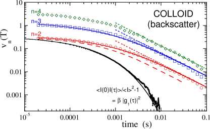
Figure 5: Reduced moments of the speckle pattern vs the exposure duration $T$, for light diffusely backscattering from an opaque colloidal suspension. Intensity autocorrelation data and fit from Fig. 2 are included for comparison. The solid curves for $n=\{2,3\}$ are generated numerically from the $g_{1}(\tau)$ data in Fig. 2 according to our theory of SVS, Eq. (15). The dotted lines represent the expected long-exposure behavior, $v_{n}(T)\sim 1/T$ of Eq. (19). The dashed curve is Eq. (24), the expectation for $v_{2}(T)$ based on the formalism of Ref. Fercher and Briers (1981).

Finally we compare with expectation based on the mistaken formalism of Ref. Fercher and Briers (1981). Introducing the correct factor of $\beta$ and taking the field autocorrelation as $g_{1}(\tau)=\exp(-\sqrt{\Gamma\tau})$, the prediction for $v_{2}(T)$ would be

$$\int_{0}^{T}\beta[g_{1}(t)]^{2}{\rm d}t/T=\beta{1-(1+2\sqrt{x})\exp(-2\sqrt{x})\over 2x},$$ (24)

where $x=\Gamma T$. This is plotted as a dashed curve for $\Gamma=1623~{}{\rm s}^{-1}$ and $\beta=0.34$, as known from the intensity autocorrelation data. Evidently, the formalism of Ref. Fercher and Briers (1981) does not correctly predict speckle variance.

IV.2 Foam

As another example, we collect SVS data for light diffusely transmitted through an aqueous foam of thickness $L=1$ cm [Gillette Foamy Regular]. The optical set-up is similar to the colloid experiments, except that the camera is moved opposite to the side upon which the laser light is incident. For this experiment, the speckles fluctuate due to sudden avalanche-like rearrangements of bubbles within small localized sub-volumes Durian et al. (1991a). Such dynamics are driven by the coarsening process, whereby small bubbles shrink and large bubbles grow in order to lower the total interfacial surface energy Durian et al. (1991b). Since the sample is far from equilibrium, and the dynamics evolve with time, we restrict data collection to a narrow time window centered at 100 minutes after production. Here the average bubble diameter is $D\approx 60~{}\mu$m, the transport-mean free path is $l^{*}\approx 3.5D$, and the average time between rearrangements at each scattering site is $\tau_{o}\approx 20$ s Durian et al. (1991b). The volume of foam sampled by the collected photons is sufficiently great that the speckle pattern is in continuous motion. The field correlation function takes the same form as for DWS in transmission from a sample of diffusing particles, $g_{1}(\tau)=\sqrt{6\Gamma\tau}/\sinh\sqrt{6\Gamma\tau}$. The first cumulant or initial decay rate is expected to be $\Gamma=(L/l^{*})^{2}/\tau_{o}\approx(1~{}{\rm cm}/0.02~{}{\rm cm})^{2}/(20~{}{\rm s})=125~{}{\rm s}^{-1}$. This understanding is supported by both single-detector Durian et al. (1991a, b); Earnshaw and Jaafar (1994); Gopal and Durian (1999) and multi-speckle Cohen-Addad and Hohler (2001); Mayer et al. (2004) dynamic light scattering experiments.

Our results for the second and third reduced moments of the distribution of pixel signals are shown in Fig. 6. For short exposures both $v_{2}(T)$ and $v_{3}(T)$ approach a constant, from which we extrapolate to zero to find $\beta=0.19$. For longer exposures, the moments become smaller as the speckle pattern fluctuates more extensively during the exposure. To model this, we numerically integrate the field correlation function $g_{1}(\tau)=\sqrt{6\Gamma\tau}/\sinh\sqrt{6\Gamma\tau}$, according to the SVS prescription of Eqs. (15). Taking the first cumulant as $\Gamma=121~{}{\rm s}^{-1}$, close to expectation, we obtain a satisfactory fit to both $v_{2}(T)$ and $v_{3}(T)$ data as shown.

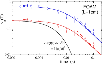
Figure 6: Reduced moments of the speckle pattern vs the exposure duration, $T$, for light diffusely transmitted through an opaque aqueous foam of thickness $L=1$ cm. The solid curves represent numerical integration of the known field autocorrelation function, $g_{1}(\tau)=\sqrt{6\Gamma\tau}/\sinh\sqrt{6\Gamma\tau}$, according to the prescription of Eq. (15). The best fit is attained for $\beta=0.19$ and $\Gamma=121~{}{\rm s}^{-1}$.

V Experimental Considerations

This final section provides guidance on the optimal design of an SVS experiment. Many of the issues, and the recommendations, are identical for other types of dynamic light scattering experiment. Throughout we shall assume that statistics are not limited by lack of photons. In this case it is advantageous to double the laser power and to place a polarizer in front of the detector. While this does not change the average detected intensity, it does improve the contrast in intensity levels at the plane of the detector, and hence the signal-to-noise, since each polarization mode forms an independent speckle pattern. Therefore, throughout, we shall assume that polarized detection is employed.

V.1 Optics

First we consider the geometry of illumination and detection. Let $a$ be the size of the region from which emerging light is collected. For single-scattering experiments this could be controlled by the diameter of the incident beam or the length it travels within the sample. For multiple-scattering experiments it could be controlled by the beam diameter or the sample thickness. The value of $a$ can also be affected by use of lenses or apertures between the sample and the detector. This is an important parameter because the angular size of the speckle, in the far field, is approximately $\lambda/a$ just as in a diffraction experiment. Thus, if the detector is located a distance $d$ away from the source of the collected light, then the speckle size or spatial correlation length is approximately $s=d\lambda/a$.

Imagining that $\lambda/a$ is fixed, and that the light intensity can be adjusted at will, we now seek to optimize the distance $d$ at which to place the detector. If $d$ is too small, then the number $N_{s}$ of speckles at each pixel will be large and the intercept, or maximum contrast, $\beta=v_{2}(0)=\langle I^{2}\rangle/\langle I\rangle^{2}-1$, will be small. The best case in terms of contrast is $\beta\rightarrow 1$ (or $\beta\rightarrow 1/2$ for unpolarized detection). In the opposite extreme, if $d$ is too large then each speckle will span many pixels and the statistics of ensemble averaging will be poor. Overall, the figure of merit to be maximized is thus $\beta\sqrt{N_{s}}$, the product of maximum contrast times the spread in number of speckles per pixel.

To find the optimal detector location by maximizing the figure of merit requires knowing $\beta$ as a function of $N_{s}$. We do this by Monte-Carlo simulation, calculating the second intensity moment across a specified area for speckle patterns generated at random with the correct statistical properties. Results for $\beta$, as well as for the figure of merit $\beta\sqrt{N_{s}}$, are plotted vs $N_{s}$ in Fig. 7. As expected, $\beta\rightarrow 1$ for small $N_{s}$ and $\beta\rightarrow 1/N_{s}$ for large $N_{s}$. The figure of merit achieves a maximum where the speckle size nearly matches the pixel size, $N_{s}=1$. As Fig. 7 demonstrates, an experiment is within about 10% of optimum if the intercept lies within the range $0.3<\beta<0.7$ (or $0.15<\beta<0.35$ for unpolarized detection). Thus a good strategy is to adjust the detector location until this criterion is met, keeping the illumination optics fixed. It is well-known that pixel and speckle sizes should be matched, but to our knowledge specific guidelines in terms of the measurable intercept have not been published.

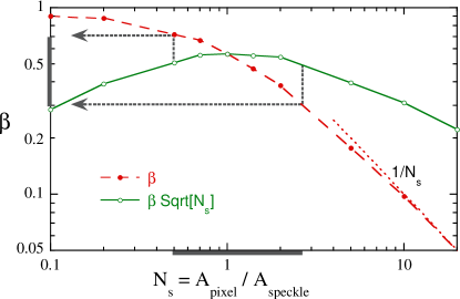
Figure 7: The intercept or maximum speckle contrast, $\beta=v_{2}(0)=\langle I^{2}\rangle/\langle I\rangle^{2}-1$, and the figure of merit $\beta\sqrt{N_{s}}$ to be maximized in design of experiment, as a function of the number $N_{s}$ of speckles per pixel. An experiment with polarized detection is within about ten percent of optimal if the intercept lies in the range $0.3<\beta<0.7$.

V.2 Light Intensity

Now we consider the optimal average intensity level, as controlled by choice of laser power. To beat photon-counting number fluctuations and dark-count subtraction error, this power should be as great as possible. However, high power can result in clipping of signal for bright speckles that exceed the maximum grayscale level of the detector. This effect introduces an error whereby the measured intensity moments are shifted systematically to lower values. In the opposite extreme, for low laser power, the detected intensity levels are binned coarsely over too few grayscale levels. This effect introduces an error whereby the moments are shifted systematically to higher values. Two other effects can introduce systematic error at low laser power. One source is dark counts. For example, the pixels of our CCD camera report fluctuating grayscale values of either 3 or 4, with a time average of 3.5, when there is no illumination. The other source of error is that the grayscale levels are reported at the lower edge of the bin, i.e. $0-255$ for an 8-bit camera like ours. For example, an actual signal level lying in the range $5\leq S<6$ is reported as a grayscale level of 5.

To investigate these effects we again turn to Monte-Carlo simulation. At first we restrict attention to an 8-bit detector with a pixel size of three speckles. This gives $\beta\approx 0.3$, and hence corresponds well with our colloid experiments. In Fig. 8 we display results for the systematic error in the first four moments as a function of average intensity level. The top plot is for an ideal detector, with zero dark counts, with signal levels taken at the lower edge of the bins, $\{0,1,2,\ldots,255\}$. Higher intensity levels are “clipped” to a value of 255. The fraction of pixels that must be clipped is plotted on the right-hand axis. At higher average intensity levels, where clipping occurs, the intensity moments fall below their correct values. At lower average intensity levels, where digitization issues occur, the intensity moments rise above their correct values. The middle plot shows that the latter can be mitigated to large extent by taking the signal level at the center of the bin. In other words, intensity moments are much more accurate if an offset of $1/2$ is added to each reported signal, so that possible levels are now $\{0.5,1.5,2.5,\ldots,255.5\}$. The bottom plot shows the effect of dark counts, as simulated by randomly adding 3 or 4 to the analog signal. This choice mimics the conditions of our colloid experiments. To mitigate both dark counts and lower-edge binning effect, we now subtract 3.5 from each pixel value. Effectively, this introduces a $\pm 1$ statistical error in pixel values, which broadens the distribution and causes higher than expected moments, as seen by comparison of Fig. 8b-c. Under the operating conditions of our colloid experiment, $\langle I\rangle=40$, we use Fig. 8c to estimate that the systematic error in our SVS data due to the combined effects of clipping, digitization, and dark-count effects is less than 0.25%.

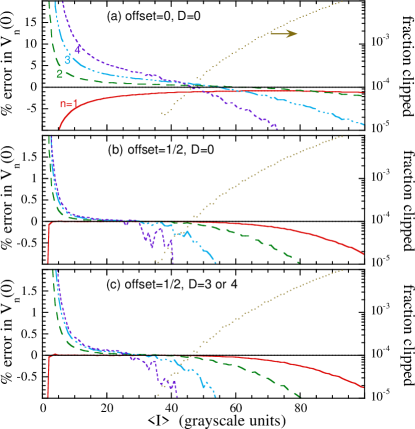
Figure 8: Simulated accuracy of SVS signals, due to errors introduced by an 8-bit digital camera, as a function of average grayscale level. For high average intensities, the brightest pixels are clipped to a grayscale level of 255; the fraction of pixels that must be clipped is shown on the right-hand axis. The top plot shows results for moments computed directly from the returned grayscale levels $\{0,1,2,\ldots,255\}$. The middle shows how the accuracy is improved dramatically if pixel values are offset by $+1/2$, which corresponds to the center of the grayscale bin. The bottom plot differs from the middle plot by inclusion of random dark counts, which are accounted for by subtraction. Note that the error scales in (b-c) are ten times smaller than the scale in (a).

We now repeat the simulations for different numbers of speckles per pixel, assuming an 8-bit camera with zero dark counts. Plots of error vs average grayscale level are used to identify a safe operating range where the error in the variance is less than 0.1%. Recommended grayscale levels are shown as a function of intercept, $\beta$, in Fig. 9. Once an optimal value of $\beta$ is achieved, for example by adjusting the detector location per the previous subsection, the laser power should be adjusted according to this plot. Photon-counting and dark-count errors can be minimized by operating at the upper end of the safe range.

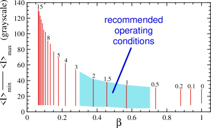
Figure 9: Recommended average intensity levels for an 8-bit digital camera, as a function of the intercept $\beta=v_{2}(0)$; the corresponding pixel area is labelled in units of average speckle area. If the average intensity is too low, then error occurs due to digitizing the intensity crudely into a small number of bins. If the average intensity is too high, then error occurs due to clipping of the high-intensity tail of the distribution. The vertical bars indicate the range over which these effects cause less than a 0.1% error in the variance. For $n$-bit cameras, the lower limit does not change but the upper limit scales with the number of grayscale levels.

V.3 Normalization factor, $\beta$

The perceived contrast of the intensity levels in a speckle pattern is reduced progressively as the pixel size increases relative to speckle size. To eliminate this effect, so that the remaining speckle contrast can serve as a quantitative probe of scattering site motion during the exposure window, the intercept $\beta\equiv v_{2}(0)=\lim_{T\rightarrow 0}(\langle I^{2}\rangle_{T}/\langle I\rangle^{2}-1)$ must be accurately determined. One approach, employed in our colloid and foam experiments above, is to collect data for many exposure times and to extrapolate the variance results to $T=0$. This is satisfactory only if the dynamics are both stationary and sufficiently slow compared to the fastest speed of the camera. Obviously another approach is needed for systems with fluctuating dynamics, where each individual exposure is to be analyzed in terms of scattering site motion at that particular moment in time. This was the case for our first reported application of SVS, where we probed grain motion as a function of phase in a vibratory oscillation cycle Dixon and Durian (2003). There we had the luxury of being able to turn off the shaking and to measure the contrast of the static speckle pattern under absolutely identical illumination and detection conditions.

Here we introduce an alternative method, whereby the value of $\beta$ can be eliminated from consideration altogether. The idea is to analyze not just one exposure, but rather some number $m$ of successive exposures all of duration $T$. The first step is to find the variance for each of the exposures, and to average the results together, giving $v_{2}(T)$. The second step is to add together the $m$ exposures pixel-by-pixel, and to compute the variance for the resulting “synthetic exposure” of duration $mT$, giving $v_{2}(mT)$. These two variances depend on the value of $\beta$, but their ratio does not:

$${v_{2}(mT)\over v_{2}(T)}={\int_{0}^{mT}[1-t/(mT)][g_{1}(t)]^{2}{\rm d}t/m\over\int_{0}^{T}(1-t/T)[g_{1}(t)]^{2}{\rm d}t}.$$ (25)

The left-hand size is thus measured, and contact with scattering site motion is made by calculation of the right-hand side for the field autocorrelation of interest. The predicted forms in Table 1 can be used directly. For short exposures or slow dynamics, the variance ratios in Eq. (25) approach one. For long exposures or fast dynamics, the variance ratios in Eq. (25) approach $1/m$. As a specific example, the variance ratio for the case of a Lorentzian spectrum, $g_{1}(\tau)=\exp(-\Gamma\tau)$, takes the form

$${v_{2}(mT)\over v_{2}(T)} = {e^{-2mx}-1+2mx\over(e^{-2x}-1+2x)m^{2}},$$ (26)

$$\approx {1+{12+2m+2m^{2}\over 15(1+m)}x+{3-2m+3m^{2}\over 15(1+m)}x^{2}\over 1+{2+2m+12m^{2}\over 15(1+m)}x+{3-2m+3m^{2}\over 15(1+m)}mx^{2}},$$ (27)

where $x=\Gamma T$ as before. The second line is a rational approximation that is correct to $O(x^{3})$ and approaches $1/m$ for long exposures. It can be inverted by solution of a quadratic equation. An additional advantage to this synthetic exposure method is that drift in laser power or detector gain, and CCD or CMOS noise that is correlated over successive exposures, are all automatically cancelled.

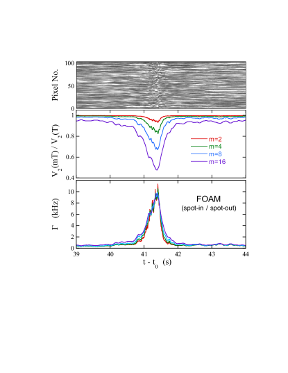
Figure 10: Pixel grayscale levels, variance ratios, and Lorentzian linewidths as a function of age for a coarsening foam. The offset along the time axis is $t_{0}=6$ hrs, the lapse between sample production and the beginning of data collection. Here the exposure duration is $T=10$ ms.

This synthetic exposure variance ratio method is now illustrated for the same coarsening foam as in Fig. 6. Here the foam is six hours old, and we employ an optical geometry whereby photons are both introduced and collected through the same 1 mm diameter aperture. This reduces the volume of foam sampled by the detected photons, and ensures that only one rearrangement event is probed at a given time. Traditional DLS methods do not apply in this regime. An example rearrangement event is captured by SVS in Fig. 10. While the bubbles remain in a fixed location, the speckle is nearly static and the variance ratios are nearly one. While the bubbles move, the speckle fluctuates and the variance ratios drop below one. According to the theory of DWS, the spectrum is Lorentzian with linewidth $\Gamma\approx 4\pi\delta v/\lambda$, where $\delta v$ is the root-mean squared ballistic speed of the rearranging bubbles. Analyzing the variance ratio data using Eq. (27) gives nearly identical linewidths for four different synthetic exposures, $m=\{2,4,8,16\}$, as shown in the bottom plot of Fig. 10. This good agreement further supports our theoretical and experimental methods of SVS. It also demonstrates how rapidly varying dynamics may now be measured.