Adiabatic pumping in a Superconductor-Normal-Superconductor weak link

Abstract

We present a formalism to study adiabatic pumping through a superconductor - normal - superconductor weak link. At zero temperature, the pumped charge is related to the Berry phase accumulated, in a pumping cycle, by the Andreev bound states. We analyze in detail the case when the normal region is short compared to the superconducting coherence length. The pumped charge turns out to be an even function of the superconducting phase difference. Hence, it can be distinguished from the charge transferred due to the standard Josephson effect.

In a mesoscopic conductor a dc charge current can be obtained, in the absence of applied voltages, by cycling in time two parameters which characterize the system thouless83 ; switkes99 . This transport mechanism is called pumping. If the time scale over which the time-dependent parameters vary is large compared to the typical electron dwell time of the system, then pumping is adiabatic, and the pumped charge does not depend on the detailed timing of the cycle, but only on its geometrical properties. Different formulations have been developed to describe adiabatic pumping, for example, based on scattering theory in Refs. brouwer98 ; makhlin01 ; buttiker02 or Green’s function methods in Refs. zhou99 ; entin02 . In the scattering approach the pumped charge per cycle can be expressed in terms of derivatives of the scattering amplitudes with respect to the pumping parameters (Brouwer’s formula brouwer98 ). This result is based on the so-called emissivities of the system buttiker94 , which express the charge that flows from a lead in response to the variation of one parameter in the scattering region. This formulation requires the presence of terminals which provide propagating channels. The scattering approach has been later extended to hybrid systems containing superconducting (S) terminals. In Refs. wang01 ; blaauboer02 a two terminal structure comprising one superconducting lead was considered. Subsequently, this approach was generalized to multiple-superconducting-lead systems, where at least one normal lead is present taddei04 . The presence of a normal lead is essential for generalizing Brouwer’s formula to these hybrid structures.

If only superconducting leads are present, at low enough temperature, pumping is due to the adiabatic transport of Cooper pairs. Besides the dependence of the pumped charge on the cycle, in the superconducting pumps there is a dependence on the superconducting phase difference(s) (the overall process is coherent). Moreover, in addition to Cooper-pair pumping, in equilibrium, there is a contribution due to the Josephson effect if the phase difference between the two superconducting leads is different from zero. Up to now adiabatic Cooper pair pumping was studied only in the Coulomb Blockade regime for all-superconducting systems (superconducting islands weakly connected to superconducting leads) geerligs91 ; pekola99 ; fazio03 ; niskanen03 . In this Letter we would like to (partially) fill this gap, and consider adiabatic pumping between two superconducting terminals connected through a normal (N) region. We focus on the regime of an open structure (SNS weak link), where charging effects are negligible. This is relevant when the normal region is, for example, a chaotic cavity as those used for normal, electronic pumps switkes99 .

The derivation of a formula for the pumped charge makes use of the connection between Berry’s phase berry84 and the pumped charge avron00 ; aunola03 ; bender05 , which we prove to be valid also for the SNS weak link. The resulting expression for the charge pumped in a period can be written in terms of derivatives of the Andreev-bound-state wavefunctions with respect to the pumping parameters. We point out that there is a close analogy of the problem studied here with that of pumping in a Aharonov-Bohm ring moskaletsring .

The system under investigation (depicted in Fig. 1) consists of a SNS junction, with the weak link occupying the region $-W/2<x<W/2$. The superconducting order parameter is given by $\Delta_{0}e^{-i\varphi/2}$ and $\Delta_{0}e^{i\varphi/2}$ for the superconductor on the left-hand-side and right-hand-side, respectively. The properties of the weak link can be varied, for example, by realizing it with a semiconductor and operating on two independent external gates, indicated by $X_{1}(t)$ and $X_{2}(t)$ in the figure.

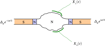
Figure 1: (Color on line.) Schematic setup for the SNS pump. The weak link is composed of a scattering region contacted to the S terminals (in orange) through two fictitious N leads (in light blue). The transport properties of the scattering region (characterized by the matrix $S_{0}$) are cycled in time via two external gates which control the parameters $X_{1}$ and $X_{2}$. The superconducting order parameters of the S terminals on the left-hand-side and on the right-hand-side have equal magnitude $\Delta_{0}$, but differ by a phase $\varphi$.

The state of such a hybrid structure $|\psi(t)\rangle$ is the solution of the time-dependent Bogoliubov-de Gennes equation:

$$i\hbar\partial_{t}|\psi(t)\rangle=H(t)|\psi(t)\rangle,$$ (1)

where the Hamiltonian

$$H(t)=\left(\begin{array}[]{cc}-\frac{\hbar^{2}}{2m}\vec{\nabla}^{2}+U(\vec{r},t)-\mu&\Delta(\vec{r})e^{i\phi(\vec{r})}\\ \Delta(\vec{r})e^{-i\phi(\vec{r})}&\frac{\hbar^{2}}{2m}\vec{\nabla}^{2}-U(\vec{r},t)+\mu\end{array}\right)$$ (2)

depends on time through the two parameters: $H(t)=H[X_{1}(t),X_{2}(t)]$. In Eq. (2) $U(\vec{r},t)$ is the potential that takes into account the effect of the time-varying external gate voltages, $\phi(\vec{r})=\varphi/2[\theta(x-W/2)-\theta(-x-W/2)]$, $\Delta(\vec{r})=\Delta_{0}/2[\theta(x-W/2)+\theta(-x-W/2)]$ and $\mu$ is the superconductor chemical potential (equal for the two S leads). We now assume that the state $|\psi(t)\rangle$ evolves adiabatically and that at any time $t$ it is in an instantaneous eigenstate of the Hamiltonian. The instantaneous solutions are defined by the equation:

$$H(t)|\tilde{\psi}(t)\rangle=\epsilon(t)|\tilde{\psi}(t)\rangle,$$ (3)

whereby $t$ plays the role of a parameter. After a cycle of period $\tau$, the states returns to the initial one, but with an added phase factor $\Phi$:

$$|\psi(\tau)\rangle=e^{i\Phi}|\psi(0)\rangle,$$ (4)

The phase $\Phi$ contains both a geometrical (Berry’s) and a dynamical contribution $\Phi=\gamma_{\text{B}}-\gamma_{\text{D}}$. The dynamical phase is simply given by $\gamma_{\text{D}}=\frac{1}{\hbar}\int_{0}^{\tau}dt\,\langle\tilde{\psi}|H|\tilde{\psi}\rangle$

For the SNS system, where Andreev bound states are formed, the condition of validity of the adiabatic approximation is that the frequency $\hbar\omega$ of the time-dependent parameters be much smaller than the energy difference between any pair of Andreev bound states, or between any Andreev bound states and the continuum of states above the gap. This implies that the pumping frequency needs at least to be smaller than the superconducting gap $\Delta_{0}$.

It is possible to show explicitly that the charge current $J_{\text{ch}}$ carried by a Bogoliubov-de Gennes eigenstate $|\tilde{\psi}\rangle$ is given by the expectation value of the derivative of the Hamiltonian $H$ with respect to the superconducting phase difference ludin99 :

$$J_{\text{ch}}=\frac{2e}{\hbar}\langle\tilde{\psi}|\frac{\partial H}{\partial\varphi}|\tilde{\psi}\rangle.$$ (5)

The charge transferred per cycle is then defined as $Q=\int_{0}^{\tau}J_{\text{ch}}(t)\,dt.$ By assuming adiabatic evolution of the state, and making use of Eq. (5), the following relation between the accumulated phase and the charge transferred in a cycle can be written:

$$Q=2e\frac{\partial}{\partial\varphi}(\gamma_{\text{D}}-\gamma_{\text{B}}).$$ (6)

The first term corresponds to the instantaneous Josephson current integrated over one period, while the second represents the pumped charge. Using Green’s theorem, $\gamma_{\text{B}}$ can be written in terms of derivatives with respect to the pumping parameter of the instantaneous eigenfunctions:

$$\gamma_{\text{B}}=-2\int_{\text{S}}dX_{1}dX_{2}\text{Im}\left[\left\langle\frac{\partial\tilde{\psi}}{\partial X_{1}}\left|\frac{\partial\tilde{\psi}}{\partial X_{2}}\right.\right\rangle\right],$$ (7)

$S$ being the area in the parameter space spanned by the parameters over one cycle. In Eq. (7) the notation $\left\langle\cdot\left|\cdot\right.\right\rangle$ stands for a space integration defined by $\left\langle A\left|B\right.\right\rangle=\int d\vec{r}\,A^{\dagger}(\vec{r})B(\vec{r})$, $A$ and $B$ being vectors in the Nambu space.

In the short junction limit (i.e. when the distance $W$ between the two superconducting interfaces is much smaller than the superconducting coherence length) only the superconducting regions contribute to the space integration in Eq. (7). The instantaneous eigenfunction, corresponding to the Andreev-bound-state energy $\epsilon_{j}$, in the superconducting regions can be written as:

$$\tilde{\psi_{j}}(\vec{r})=\left\{\begin{array}[]{lr}\tilde{\psi}_{\text{S,L},j}(\vec{r})&x\leq-W/2\\ \tilde{\psi}_{\text{S,R},j}(\vec{r})&x\geq W/2\end{array}\right.,$$ (8)

with

$$\tilde{\psi}_{\text{S,L},j}(\vec{r})=\sum_{n}\left(\mathbf{b}^{+}_{\text{L}n,j}e^{-ik^{+}_{n,j}x}+\mathbf{b}^{-}_{\text{L}n,j}e^{ik^{-}_{n,j}x}\right)\chi_{n}(y,z)$$ (9)

and

$$\tilde{\psi}_{\text{S,R},j}(\vec{r})=\sum_{n}\left(\mathbf{b}^{+}_{\text{R}n,j}e^{ik^{+}_{n,j}x}+\mathbf{b}^{-}_{\text{R}n,j}e^{-ik^{-}{{}_{n},j}x}\right)\chi_{n}(y,z),$$ (10)

$n$ being the transverse channel index relative to the transverse wavefunction $\chi_{n}(y,z)$ with transverse subband energies $E_{n}$ note0 . The index $j$ labels the different Andreev bound states. In Eqs. (9) and (10) $k^{\pm}_{n,j}$ are particle(hole)-like quasiparticle wavevectors given, in the Andreev approximation ($\Delta_{0}\ll\mu-E_{n}$ for any $E_{n}$), by $k^{\pm}_{n,j}=k_{\text{F}n}\left(1\pm\frac{i}{2}\sqrt{\frac{\Delta^{2}_{0}-\epsilon_{j}^{2}}{(\mu-E_{n})^{2}}}\right)$, with $k_{\text{F}n}=\sqrt{\frac{2m}{\hbar^{2}}(\mu-E_{n})}$. The Nambu-space vectors $\mathbf{b}^{\beta}_{\nu n,j}$ can be calculated with the following procedure: i) the eigenfunction in the fictitious leads in the normal regions adjacent to the superconducting interface (see Fig. 1) are calculated along the lines of Ref. beenakker92 ; ii) the wavefunction in the superconductor is obtained by imposing the continuity equations at the interfaces within the Andreev approximation; iii) the normalization condition $\sum_{\nu=\text{L,R}}\left\langle\tilde{\psi}_{\text{S},\nu,j}\left|\tilde{\psi}_{\text{S},\nu,j}\right.\right\rangle=1$ is imposed.

Making use of the Andreev approximation, the pumped charge reduces to

$$Q_{\text{p }}=4e\frac{\partial}{\partial\phi}\int_{\text{S}}dX_{1}dX_{2}\sum_{\stackrel{{\scriptstyle{\stackrel{{\scriptstyle\beta=+,-}}{{\nu=\text{L,R}}}}}}{{n,j}}}\left\{\frac{1}{2\text{Im}k^{+}_{n,j}}\text{Im}\left[\frac{\partial\mathbf{b}_{\nu n,j}^{\beta\dagger}}{\partial X_{1}}\frac{\partial\mathbf{b}_{\nu n,j}^{\beta}}{\partial X_{2}}\right]+\frac{1}{(2\text{Im}k^{+}_{n,j})^{2}}\text{Re}\left[\mathbf{b}^{\beta\dagger}_{\nu n,j}\frac{\partial\mathbf{b}^{\beta}_{\nu n,j}}{\partial X_{2}}\frac{\partial k^{+}_{n,j}}{\partial X_{1}}+\frac{\partial\mathbf{b}^{\beta\dagger}_{\nu n,j}}{\partial X_{1}}\mathbf{b}^{\beta}_{\nu n,j}\frac{\partial k^{+}_{n,j}}{\partial{X_{2}}}\right]\right\},$$ (11)

where the sum over $j$ runs over the Andreev bound states. This is the central result of this Letter, and a few comments are in order. We have succeeded in expressing the pumped charge as a function of the instantaneous Andreev-bound-state eigenfunction. The vectors $\mathbf{b}^{\pm}_{\text{L(R)}n,j}$ depend only on the parameters of the system, such as the normal region scattering matrix $S_{0}$, the superconducting gap, and the superconducting phase difference. It is clear that the pumped current can be written in terms of the elements of the normal-region scattering matrix $S_{0}$. Equation (11) is a zero temperature result, and contains only the contribution to the pumped charge due to the Andreev bound states. At finite temperatures, but still smaller than the gap, the contributions of the different Andreev bound states $\epsilon_{j}$ are weighted by the thermal occupation $1-2f(\epsilon_{j})$, being $f$ the Fermi function. At temperatures of the order of the gap, there is an additional contribution, not contained in Eq. (11), due to the propagating quasi particles with energies above the gap. When superconductivity is suppressed only the latter contribution, which is described by Brouwer’s formula, remains, leading to the usual result for the pumped charge through a normal region connected to normal leads.

Now let us consider the following single-channel parametrization for the normal-conductor scattering matrix

$$S_{0}=\left(\begin{array}[]{cc}e^{i\alpha}\sqrt{1-g}&i\sqrt{g}\\ i\sqrt{g}&e^{-i\alpha}\sqrt{1-g}\end{array}\right),$$ (12)

choosing $g$ and $\alpha$ as pumping fields ($X_{1}=g$, and $X_{2}=\alpha$). The instantaneous Andreev-bound-state energy $\epsilon_{0}$ is simply related to the transmission probability $g$ by beenakker92

$$\epsilon_{0}(t)=\Delta_{0}\sqrt{1-g(t)\sin^{2}(\frac{\varphi}{2})},$$ (13)

so that $\gamma_{\text{D}}=1/\hbar\int_{0}^{\tau}\epsilon_{0}(t)$.

The charge transfered due to the Josephson current (in the following named also Josephson charge) reads

$$Q_{\text{Jos}}=-2e\frac{\Delta_{0}}{\hbar}\int_{0}^{\frac{2\pi}{\omega}}dt\,\,\,\frac{g(t)}{2}\frac{\sin{\left(\frac{\varphi}{2}\right)}\cos{\left(\frac{\varphi}{2}\right)}}{\sqrt{1-g(t)\sin^{2}{\left(\frac{\varphi}{2}\right)}}}.$$ (14)

Notice that it depends on the pumping frequency $\omega$. On the other hand, the pumped charge does not depend on the pumping frequency, but only on the geometrical properties of the pumping cycle, and it reads

$$Q_{\text{p}}=4e\int_{S}dgd\alpha\frac{\partial}{\partial\varphi}\text{Im}\left[\left\langle\frac{\partial\tilde{\psi}}{\partial g}\left|\frac{\partial\tilde{\psi}}{\partial\alpha}\right.\right\rangle\right].$$ (15)

Interestingly, the integrand of Eq. (15) turns out to be independent of $\alpha$.

We now consider the following sinusoidal pumping cycle: $g(t)=\bar{g}+\Delta g\sin(\omega t)$ and $\alpha(t)=\bar{\alpha}+\Delta\alpha\sin(\omega t+\phi_{0})$. In the weak pumping limit we assume that $\Delta g/\bar{g}\ll 1$ so that the integrand of Eqs. (14) and (15) vary negligibly during the cycle. As far as the frequency is concerned, the maximum value of $\hbar\omega$ in order for the adiabatic hypothesis to hold is $\hbar\omega<\Delta_{0}-\bar{\epsilon}_{0}$, with $\bar{\epsilon}_{0}=\Delta_{0}\sqrt{1-\bar{g}\sin^{2}(\varphi/2)}$. In order to compare $Q_{\text{p}}$ with $Q_{\text{Jos}}$, we choose $\hbar\omega=0.1(\Delta_{0}-\tilde{\epsilon}_{0})$, $\tilde{\epsilon}_{0}$ being equal to the value of $\bar{\epsilon}_{0}$ at $\varphi=\pi/2$. Note that the adiabatic condition breaks down for $\varphi=0$ or $\bar{g}=0$, when the Andreev bound state is at the gap boundary. Thus in our analysis we shall avoid small values of those variables.

Figure 2 shows the pumped charge as a function of the superconducting phase difference $\varphi$ for different values of $\bar{g}$. $Q_{\text{p}}$ is a non-monotonous function of $\varphi$ exhibiting a maximum at $\varphi=\pi$. For comparison, in the inset of Fig. 2, we plot the transferred charge due to the Josephson current, whose absolute value is larger, with respect to the pumped current, by a factor of order $\hbar\omega/\Delta_{0}$. However, while $Q_{\text{p}}(\varphi)$ is an even function of $\varphi$, $Q_{\text{Jos}}(\varphi)$ is odd, so that a measure of $[Q(\varphi)+Q(-\varphi)]/2$ will single out only the pumped contribution. The particular parity of $Q_{\text{p}}$ is due to the fact that a time-reversal operation implies not only the reversal of phase but also of the pumping trajectory in parameter space. It has also to be noticed (see Fig. 2) that the pumped charge is not quantized. In absence of Coulomb blockade, charge quantization occurs only for very specific pumping cycles (see, for example, Ref. makhlin01 ). In addition the global superconducting phase-coherence of the system, which leads to wave functions extending in the two superconducting electrodes, also hinders charge quantization.

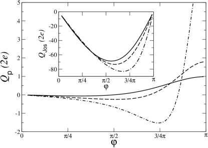
Figure 2: Pumped charge, in units of $2e$, as a function of superconducting phase difference $\varphi$ computed for a sinusoidal weak-pumping cycle. Different lines refer to different values of average transmission: solid line $\bar{g}=0.5$; dashed line $\bar{g}=0.7$; and dot-dashed line $\bar{g}=0.9$. For the pumping cycle we have chosen $\Delta g=0.1$, $\Delta\alpha=2\pi$ and $\hbar\omega=0.1\Delta_{0}(1-\sqrt{1-\bar{g}/2})$. In the inset the Josephson charge is plotted as a function of $\varphi$ for the same parameters of the main panel.

To study the effect of an external magnetic field in the normal region, we change slightly the parametrization of $S_{0}$ introducing a phase factor $\exp{\pm i\beta}$ in the transmission amplitudes. As a result both the pumped and the Josephson charge are shifted along the $\varphi$ axis by $2\beta$, i.e. $Q_{\text{p/Jos}}(\varphi)\rightarrow J_{\text{p/Jos}}(\varphi-2\beta)$. For example, the maximum pumped charge is now reached for $\varphi=2\beta-\pi$.

As far as detection is concerned, we wish to stress that for realistic parameters, using Al as superconductor, one can attain sizable pumped currents of the order of 5 nA. A sensitive setup to currents of even smaller size can be realized by inserting the SNS pump in a arm of a SQUID.

In conclusion, we have presented a formalism to study adiabatic charge pumping in a SNS weak link. The pumped charge is related to the Berry’s phase accumulated in a pumping cycle by the Andreev bound-state wavefunctions, which can be written as a function of the scattering matrix of the normal region. In the short junction limit, the pumped charge is even with respect to the superconducting phase difference. Hence, it can be easily distinguished from the charge transferred by the Josephson current.

- (1) D.J. Thouless, Phys. Rev. B 27, 6083 (1983).
- (2) M. Switkes, C.M. Marcus, K. Campman, and A.C. Gossard, Science 283, 1905 (1999).
- (3) P.W. Brouwer, Phys. Rev. B 58, R10135 (1998).
- (4) Yu. Makhlin and A.D. Mirlin, Phys. Rev. Lett. 87, 276803 (2001).
- (5) M. Moskalets, and M. Büttiker, Phys. Rev. B 66, 035306 (2002).
- (6) F. Zhou, B. Spivak, and B. Altshuler, Phys. Rev. Lett. 82, 608 (1999).
- (7) O. Entin-Wohlman, A. Aharony, and Y. Levinson, Phys. Rev. B 65, 195411 (2002).
- (8) M. Büttiker, H. Thomas, and A. Prêtre, Z. Phys. B 94, 133 (1994).
- (9) J. Wang, Y. Wei, B. Wang, and H. Guo, Appl. Phys. Lett. 79, 3977 (2001).
- (10) M. Blaauboer, Phys. Rev. B 65, 235318 (2002)
- (11) F. Taddei, M. Governale, and R. Fazio, Phys. Rev. B 70, 052510 (2004).
- (12) L.J. Geerligs et al., Z. Phys. B 85, 349 (1991).
- (13) J.P. Pekola, J.J. Toppari, M. Aunola, M.T. Savolainen, and D.V. Averin, Phys. Rev. B 60, R9931 (1999).
- (14) R. Fazio, F.W.J. Hekking, and J.P. Pekola, Phys. Rev. B 68, 054510 (2003).
- (15) A.O. Niskanen, J.P. Pekola, and H. Seppä, Phys. Rev. Lett 91, 177003 (2003).
- (16) M.V. Berry, Proc. R. Soc. London A 392, 45 (1984).
- (17) J.E. Avron, A. Elgart, G.M. Graf, and L. Sadun, Phys. Rev. B 62 R10618 (2000).
- (18) M. Aunola and J.J. Toppari, Phys. Rev. B 68, 020502 (2003).
- (19) A. Bender, F.W.J. Hekking, and Yu. Gefen, (unpublished).
- (20) M. Moskalets, and M. Büttiker, Phys. Rev. B 68, 075303 (2003).
- (21) N. I. Ludin, L. Y. Gorelik, R. I. Shekhter, M. Jonson, and V. S. Shumeiko, Superlattices and Microstructures 25, 937 (1999).
- (22) Equations (9) and (10) are valid in general. However, beyond the short-junction limit the knowledge of the wave function in the normal region is necessary to compute the space integration in Eq. (7).
- (23) C.W.J. Beenakker, in Transport Phenomena in Mesoscopic Systems, Eds. H. Fukuyama, and T. Ando, Springer Series in Solid-State Sciences, vol. 109 (Springer-Verlag, Berlin Heidelberg 1992), p. 235.