The partition of energy for air-fluidized grains

Abstract

The dynamics of one and two identical spheres rolling in a nearly-levitating upflow of air obey the Langevin Equation and the Fluctuation-Dissipation Relation [Ojha et al. Nature 427, 521 (2004) and Phys. Rev. E 71, 016313 (2005)]. To probe the range of validity of this statistical mechanical description, we perturb the original experiments in four ways. First, we break the circular symmetry of the confining potential by using a stadium-shaped trap, and find that the velocity distributions remain circularly symmetric. Second, we fluidize multiple spheres of different density, and find that all have the same effective temperature. Third, we fluidize two spheres of different size, and find that the thermal analogy progressively fails according to the size ratio. Fourth, we fluidize individual grains of aspherical shape, and find that the applicability of statistical mechanics depends on whether or not the grain chatters along its length, in the direction of airflow.

I Introduction

There is a growing list of driven, far-from-equilibrium systems where the dynamics of microscopic fluctuations are characterized by an effective temperature. One of the earliest examples is the kinetic energy associated with velocity fluctuations in a sheared granular material Bagnold (1954). More recent examples in granular physics include dilute grains driven within a horizontal planePouligny et al. (1990); Ippolito et al. (1995); Prentis (2000); Ojha et al. (2004, 2005), as well as flowing granular liquids Menon and Durian (1997); Mueth et al. (2000); Losert et al. (2000); Reydellet et al. (2000); Lemieux and Durian (2000); Song et al. (2005) and vertically-vibrated granular gasses Olafsen and Urbach (1998); Feitosa and Menon (2002); D’Anna et al. (2003); Baxter and Olafsen (2003). Wider ranging examples include chaotic fluids Hohenberg and Shraiman (1989); Egolf (2000), spin glasses Cugliandolo and Kurchan (1993); Herisson and Ocio (2002), glasses Grigera and Israeloff (1999); Berthier and Barrat (2002), colloids Segre et al. (2001); Bellon et al. (2001), and foams Ono et al. (2002), which are all far away from equilibrium. In some of these cases Prentis (2000); Ojha et al. (2004); Song et al. (2005); D’Anna et al. (2003); Baxter and Olafsen (2003); Ono et al. (2002), the behavior is in perfect analogy with that expected for a system in thermal equilibrium. Degrees of freedom are populated according to a density of states and Boltzmann factor, and correlation-response relations all hold, with a single effective temperature whose value is set by the nature of the energy injection mechanism. In other cases, such a thermal analogy is more limited and does not hold in detail; for example, the distributions may not be described by a Boltzmann factor or the effective temperature may not be uniquely defined.

An outstanding question is how to predict whether or not the thermal analogy holds. What do the systems in Ref. Prentis (2000); Ojha et al. (2004, 2005); Song et al. (2005); D’Anna et al. (2003); Baxter and Olafsen (2003); Ono et al. (2002) have in common, and how do they differ from other driven systems? Here we seek insight by systematically perturbing one case for which the analogy unarguably holds in all detail, in hopes that it may be progressively upset. In particular, we focus on a small number of grains fluidized in a nearly-levitating upflow of air. While grains thus never leave the plane, they can nevertheless be driven randomly within the plane by the random shedding of turbulent wakes at a rate set by the Strouhal number Achenbach (1974); Suryanarayana and Prabhu (2000). The Reynold’s number based on sphere size is of order $10^{4}$. Under these conditions, a single sphere confined within a circular cell rolls stochastically, without slipping, exactly like a Brownian particle in a two-dimensional harmonic trap Ojha et al. (2004). Specifically, the dynamics obey a Langevin equation where the random force autocorrelation is proportional to the viscous drag memory kernel and the effective temperature according to the Fluctuation-Dissipation Relation. For a variety of conditions, the root-mean-squared displacement of the sphere from the center of the trap and the mean-squared speed of the sphere, respectively, are given by Ojha et al. (2005)

$$\sqrt{\langle r^{2}\rangle} = (0.20\pm 0.02)R_{cell},$$ (1)

$$\langle v^{2}\rangle = 0.7\left({\rho_{air}\over{\rho_{e}}}\right){u^{3}\over\sqrt{gD}}.$$ (2)

Here $\rho_{e}=m_{e}/[(4/3)\pi(D/2)^{3}]$; $m_{e}=m+I/(D/2)^{2}$ is the effective inertial mass of the sphere; $m$, $I$, and $D$ are respectively the mass, moment of inertia and diameter of the sphere; $\rho_{air}$ and $u$ are respectively the density and flow speed of the air; $g=980~{}{\rm cm/s^{2}}$ is gravitational acceleration; and $R_{cell}$ is the radius of the sample cell. Physically, Eq. (2) can be understood by balancing energy input, via collision between the sphere and a sphere-sized volume of air, with energy dissipation via viscous drag. Geometrically, Eq. (1) can be understood by a picture of the repulsion between the cell wall and the turbulent wake, which expands as it moves downstream.

The detailed thermal analogy for the behavior of one and two nearly-levitated gas-fluidized spheres was completely unexpected. In this paper, we seek insight via systematic perturbation of the original experiment. To begin, we first describe the experimental apparatus and analysis procedures used throughout. In the next four sections, we describe the perturbations and results, with one perturbation per section. We shall demonstrate that the thermal analogy is very robust with respect to some of these perturbations. We also shall demonstrate a control parameter by which the thermal analogy may be progressively upset.

II Experimental Details

Our methods for fluidizing grains and tracking their positions are similar to those of Refs. Ojha et al. (2004, 2005), but with some embellishments that we describe in detail here. As before, the heart of the apparatus is a rectangular windbox, $1.5\times 1.5\times 4~{}{\rm ft}^{3}$, standing upright. A circular sieve with mesh-size 300 $\mu$m sits in a twelve-inch circular hole on the top. The sieve is horizontal, so that the grains feel no component of gravity within the plane of motion and so that the air flow is upward counter to gravity. Except in the final section, all grains are spherical and roll without slipping. The rotational motion is therefore coupled to the translational motion and can be accounted for by an effective inertial mass as in Eq. (2). A digital CCD video camera [Pulnix 6710, 8 bits deep, 120 Hz frame rate], and a ring of six 100 W incandescent lights, are located approximately three feet directly above the sieve, mounted to a scaffolding which in turn is mounted to the windbox. A blower is connected at the base of the windbox to provide an upward air flow perpendicular to the sieve. A hotwire anemometer measures the flow rate, and verifies its uniformity. Previously, a perforated metal sheet was fixed in the middle of the windbox to break up large scale structures in the airflow. To ensure even more uniformity, we now use two perforated metal sheets with a one-inch thick foam air-filter sandwiched in between.

The control of the camera, and all image processing, is accomplished within LabVIEW. In all runs, images are harvested at 120 frames per second and written to hard disk for post processing. To minimize the size of the data set, and hence to optimize the maximum possible run length, we first threshold the images to binary so that each grain appears as a white blob on a black background. The illumination and thresholding level are adjusted so that each blob corresponds closely to the entire projected area of the grain. Successive binary images are encoded as a lossless format AVI movie [Microsoft RLE]. Previously, we used a custom encoding scheme that is optimal only for a very small number of spherical grains. The AVI format requires more disk space, but is also more flexible for large numbers of grains.

For post-processing we also use LabVIEW. If the grains are far enough apart as to be distinct white blobs that are completely surrounded by black, then we use LabVIEW’s “IMAQ Particle Analysis” algorithm to locate the center of brightness of each blob to sub-pixel accuracy. However, when two grains collide and their blobs touch, then this algorithm identifies only the center of the combined two-grain blob. When the total number of identified blobs falls below the known number of grains, we must modify our tracking procedure. The widely-used technique of Ref. Crocker and Grier (1996) cannot be invoked, because it requires the grain separation be large compared to grain size. Instead, we apply an erosion algorithm, in which a square mask consisting of ones (white) and zeros (black) is run over the binary image. The output at each pixel is one (white) if all the image pixels under the white region of the mask are white; otherwise, the output is zero (black). For spherical grains, we choose a mask that is about 2/3 the grain size, that is white throughout the largest inscribed circle, and that is black outside this region. This construction preserves the circular shape of the blobs, while eroding their size. It also separates blobs that are in contact, and optimizes their circularity after separation. After applying such an erosion, we then invoke the same centroid-finding algorithm as before. These procedures are demonstrated in Fig. 1, which shows two grains before, during, and after collision.

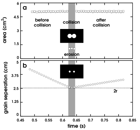
Figure 1: [col-ero] (a) The measured blob area, and (b) the center-to-center separation, for two grains in collision. The grayed stripe indicates the time-interval the grains are in close enough proximity so that they are imaged as as a single blob (inset a), which is eroded producing two smaller separated circles (inset b).

There are two more steps. First, the grain coordinates measured in each frame must be identified with the correct corresponding grains in the previous frame. This is aided by the fast frame rate of our camera, which is such that the maximum displacement in one frame is much less than the grain size. Finally, position vs time data is fitted to a third order polynomial within a window of $\pm 5$ points in order both to smooth and to differentiate to second order. Gaussian weighting that is nearly zero at the edges is used to ensure continuity of derivatives. The rms deviation of the raw data from the polynomial fit is 0.001 cm, which we take as an estimate of position accuracy. This and the frame rate give an estimate of speed accuracy as 0.1 cm/s. Indeed these numbers correspond to a visual inspection of the level of noise in time traces.

III One sphere in a stadium

Our first perturbation is motivated by the very form of Eq. (1), which says that the rms position of the sphere is set by the radius of the sieve. So instead of using a circular sample cell, we now construct a stadium-shaped sample cell by placing appropriate wooden inserts into contact with the sieve both above and below. A binary image of our stadium, with a $D=1$ inch nylon sphere, is shown in the inset of Fig. 2. Certainly the elongated boundary will affect the confining ball-wall potential, with the sphere expected to move farther along the long axis. Due to loss of symmetry, the rms position and speed of the grain could now both be different along the long and short axes, which would be a direct violation of the thermal analogy. To investigate, we fluidize the nylon ball with an upflow of air at speed $u=750$ cm/s, and we track its position with the methods described above.

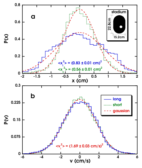
Figure 2: [v-p-dis] Distributions for the components of (a) position and (b) velocity measured for a one-inch nylon sphere along the long and short axes of a stadium-shaped trap. To within measurement uncertainty, these distributions are all Gaussian (dashed curves).

Results for the position and speed distributions along the two axes of the stadium are displayed in Fig. 2. All four have the same Gaussian shape, characteristic of a Brownian particle in a harmonic trap, as seen before. Though it couldn’t have been expected, the speed distributions remain identical along the two axes. However, the sphere now has wider excursions along the longer axis. The observed rms displacements are $\sqrt{\langle{x_{l}}^{2}\rangle}=0.83$ cm and $\sqrt{\langle{x_{s}}^{2}\rangle}=0.56$ cm for long and short axes, respectively. The ratio of these displacements is 1.48, which is very close to the ratio of long to short dimensions of the stadium, (22.8 cm)/(15.2 cm)=1.50, in accord with the scaling of Eq. (1).

If the thermal analogy holds for both the position and momentum degrees of freedom, then the spring constants along the two axes can be deduced from the equipartition of energy:

$$T\ =m_{e}\langle{v_{l}}^{2}\rangle=m_{e}\langle{v_{s}}^{2}\rangle=k_{l}\langle{x_{l}}^{2}\rangle=k_{s}\langle{x_{s}}^{2}\rangle,$$ (3)

where $T$ is the effective temperature measured in units of energy. To test this relation, we compare with an auxiliary mechanical measurement of the spring constants. As in Ref. Ojha et al. (2004), we tip the entire apparatus by a small angle $\theta$ away from horizontal and measure the shift $\langle\Delta x\rangle$ in the average position of the sphere down the plane. The new average position is where the spring force balances the force of gravity acting within the plane:

$$k\langle\Delta x\rangle=mg\sin\theta.$$ (4)

This is done for orientations of the stadium with the long axis both parallel and perpendicular to the tilting direction. The results for the shift in average position are plotted as symbols vs the sine of the tilt angle in Fig. 3. The expectations based on Eq. (3) and the position and speed statistics are also plotted in Fig. 3, now as a shaded region that reflects measurement uncertainty in the rms displacements and speeds. Indeed, the two results agree well.

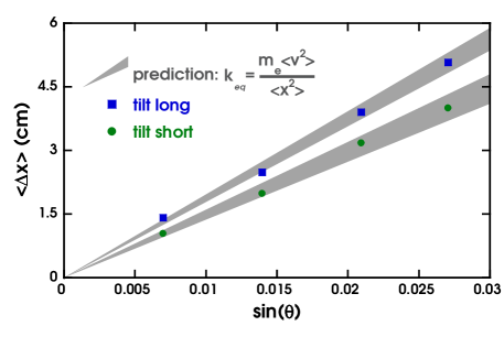
Figure 3: [spr-cons] Shift in average position of a fluidized sphere with respect to the sine of the angle by which the entire apparatus is tilted. Data are shown by symbols, and prediction based on the equipartition assumption and the variance of the position and speed distributions are shown by shaded regions. The experimental conditions are the same as in Fig. 2.

To drive home the validity of the thermal analogy for a nearly-levitated sphere in a stadium-shaped cell, we now compute the total mechanical energy $E$ as the sum of kinetic and potential energies at each instant in time. We then compute the distribution of total energy sampled over the entire run. The data, shown in the main plot of Fig. 4, agree nicely with the expectation for a thermal system, $P(E)=(E/T^{2})\exp(-E/T)$, which is given by the density of states times the Boltzmann factor with no adjustable parameters. The insets show no correlation in phase-space scatter plots of speed vs position.

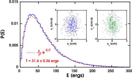
Figure 4: [ene-dis] The energy distribution for a one-inch nylon sphere in a stadium-shaped trap, under the same conditions as in Figs. 1-2. The dashed curve shows the expectation based on the known effective temperature and the product of density of states times a Boltzmann factor. The insets show scatter plots of velocity and position components; successive points are separated by several seconds, longer than the decay time of the velocity autocorrelation function.

While we might have hoped to tune the validity of the thermal analogy by the value of the aspect ratio of the sample boundary, apparently it is robust with respect to this perturbation and we must look elsewhere.

IV Five spheres of different density

Our second perturbation is motivated by the form of Eq. (2), which specifies the mean-squared speed of individually fluidized spheres as a function of the air and sphere properties. Note that Eq. (2) gives the scaling of the mean kinetic energy with sphere density as $K\sim 1/\rho_{e}$, due to the way energy is injected by turbulent wakes. If this relation also holds when multiple spheres of different density are in the sample cell, then the spheres would have different temperatures. To test this possibility we now simultaneously fluidize five solid spheres of the same diameter, $D=2.54$ cm, but of different density. The materials and effective densities of the spheres are as follows: wood 0.95 g/cc; polypropylene 1.29 g/cc; nylon 1.57 g.cc; teflon 3.02 g/cc; Al₂O₃ ceramic 5.33 g/cc. We note that the wooden ball is slightly aspherical, and its diameter is about 0.5% smaller than the others. The air speed is $u=600$ cm/s, the trap is circular, and the sieve is perpendicular to gravity.

The normalized speed distributions are displayed in Fig. 5 for the five spheres. All have the same Gaussian form as for a thermal particle in two dimensions, $P(v)=(2v/\langle v^{2}\rangle)\exp(-v^{2}/\langle v^{2}\rangle)$. But evidently the lighter spheres move faster, on average, than the denser spheres. The mean kinetic energy for each sphere is plotted in Fig. 6 vs effective density. There is a slight upward trend, with a difference of about thirty percent from lightest to densest spheres. This rise is slightly larger that the measurement uncertainty. More crucially, it is also slight in comparison with the factor of five decrease predicted by Eq. (2) for one ball alone, $K\sim 1/\rho_{e}$; Eq. (2) can be completely ruled out for multi-ball systems. Apparently the spheres exchange energy, mainly through interaction of their wakes as well as through occasional direct collisions, and thereby come to almost the same temperature. The thermal analogy is fairly robust with respect to perturbation of sphere density.

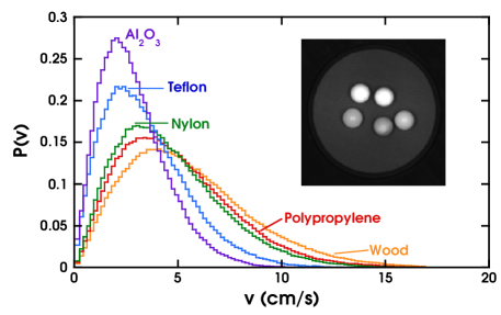
Figure 5: [diffdens] Speed distributions for grains of equal diameter but different density. In order of decreasing density, the sphere materials are ceramic (Al₂O₃), Teflon, Nylon, polypropylene, and wood. The inset shows a photograph of the system.

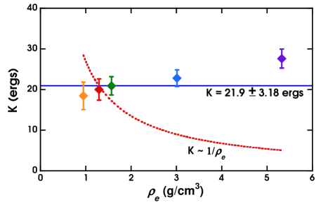
Figure 6: [ener] Average kinetic energy vs density, based on the speed distributions shown in Fig. 5 for five spheres of equal diameter. To within measurement uncertainty, the results are nearly constant, as shown by the solid horizontal line. The expectation based on single-grain behavior, Eq. (2), is shown by a dashed curve.

V Two spheres of different size

Our next perturbation is also motivated by the form of Eq. (2), which implies that the mean kinetic energy of an individually fluidized sphere scales with sphere diameter as $K\sim D^{5/2}$. If this holds when multiple spheres of different diameter are simultaneously fluidized, then the spheres would have different temperatures. To test this possibility, we fluidize pairs of nylon spheres of different diameter. The airspeed is $u=770$ cm/s and the trap is circular. By varying the choice of spheres, we have examined the behavior for seven diameter ratios ranging from about 0.5 to 5.

The speed distributions are always nearly Gaussian. This is quantified in Fig. 7a, which shows the kurtosis $\langle v^{4}\rangle/\langle v\rangle^{4}$ of the speed distribution for each sphere as a function of diameter ratio. The values are close to 3, the Gaussian expectation, except for two cases. This in and of itself is a violation of the thermal analogy. However, it is not so drastic that the mean kinetic energy, and hence the effective temperature, become ill-defined.

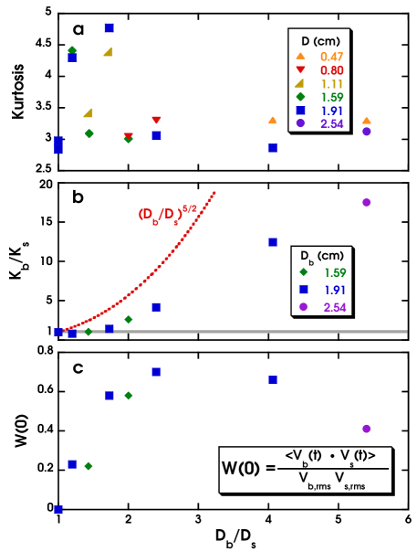
Figure 7: [TRK] (a) Kurtosis of the velocity distributions, (b) ratio of average kinetic energies, and (c) equal-time velocity cross-correlation for pairs of nylon spheres vs the ratio of their diameters. For the thermal analogy to hold, the kurtosis should equal 3, the kinetic energy ratio should equal 1, and the equal-time velocity cross-correlation should vanish. The ratio of average kinetic energies predicted by single-sphere behavior, Eq. (2), is shown by a dashed curve.

The ratio of mean kinetic energies of the two balls, which equals the ratio of their effective temperatures, is plotted vs diameter ratio in Fig. 7b. The kinetic energies are nearly equal for diameter ratios of less than two. But for increasing diameter ratio, the larger sphere becomes progressively hotter than the smaller sphere. Evidently, the diameter ratio is a control parameter that can be varied to systematically break the thermal analogy. This breakdown appears to be quite gentle, though. The temperature ratio is not as great as expected by Eq. (2), which again we find to be incorrect for multi-ball systems. Also, the leading behavior is not linear, but rather quadratic in the diameter ratio. This may be amenable to theoretical modelling.

Before closing this section, we now consider the physical origin of the breakdown of the thermal analogy vs diameter ratio. The reason, actually, is immediately obvious when viewing the system directly. The two spheres usually repel one another through interaction of their wakes, as discussed in Ref. Ojha et al. (2005). However, if they approach close enough, then they come into lasting contact and the upflow of air exerts a net total force on the pair causing them to accelerate straight across the cell until reaching the boundary. The direction of motion is such that the large sphere appears to chase the small sphere out of its territory. We speculate that the loss of symmetry of the two-ball pair causes the vortices to be shed preferentially along the line of centers, resulting in a net force.

The prevalence of this “chasing”phenomenon may be quantified by the equal-time velocity cross-correlation, $\langle{\bf v_{b}}(t)\cdot{\bf v_{s}}(t)\rangle$, where the subscripts denote “big” and “small” spheres as before. For the thermal analogy to hold, this quantity must vanish because all kinetic degrees of freedom must be independently populated. During a chase, however, the two velocities are equal and hence perfectly correlated. Data for the equal-time velocity cross-correlation, made dimensionless by the rms speeds of the two balls, are plotted vs diameter ratio in Fig. 7c. By contrast with the effective temperature ratio, this rises abruptly from zero for diameter ratios greater than one. Also by contrast, it reaches a peak for a diameter ratio of about 3 and then decreases. If the size disparity is too small, then the loss of symmetry is not enough to cause much chasing. If the size disparity is too great, then the large grain slowly rolls without regard for the small ball, which quickly flits about and is repelled as though from a stationary object. We believe the thermal analogy is recovered in this limit, but with the two balls being differentially “heated” by the upflow of air.

VI One aspherical grain

In the above sections, and also in Refs. Ojha et al. (2004, 2005), the shape of the grain is spherical. This is special because it permits the grain to roll freely in all directions without sliding. It is also special because it permits vortices to be shed equally in all directions. To explore for qualitatively new phenomena, and to seek another means of violating the thermal analogy, we now perturb the grain shape. The objects we fluidize are listed in Table 1 and pictured in Fig. 8: various pharmaceutical pills, a cylindrical wooden rod, and a dimer consisting of two connected hollow plastic spheres. When individually fluidized by an upflow of air, the pictured grains all translate and rotate seemingly at random. A few of the grains are axisymmetric, like the dimer; however, they exhibit virtually no rotation about the axis of continuous symmetry. While the spheres in previous sections roll without slipping, here the aspherical grains must slide in order to translate or rotate.

We may characterize the motion of these grains in terms of the time dependence of their center-of-mass position and their angular orientation. The former is deduced as per the spherical grains from the center of brightness. The latter is deduced from second moments of the spatial brightness distribution. Then we differentiate to measure both translational and rotational speed distributions. None of the grains is chiral by design, since that would lead to steady whirling in one direction. Nonetheless, some whirling can occur due to imperfections in shape. Therefore we measure both the average angular speed $\langle\omega\rangle$ as well as fluctuations $\delta\omega$ about this average.

Name	$\rho$ (g/cc)	$L$ (cm)	$W$ (cm)	$H$ (cm)	$m$ (g)	$I$ (g-cm2)
white	0.685	2.12	0.848	0.848	0.82	0.344
silver	0.951	1.52	0.586	0.586	0.39	0.083
brown	0.937	1.94	0.966	0.888	1.56	0.611
wood	0.671	4.75	0.540	0.540	0.73	1.386
dimer	0.256	5.08	2.540	2.540	4.40	11.34

Table 1: The density, length, width, height, mass, and moment of inertia of five aspherical grains. For computation of density and moment of inertia, the white, silver, and wood grains are approximated as cylinders, while the brown grain is approximated as a block. The dimer is composed of two polypropylene shells of thickness 0.14 cm.

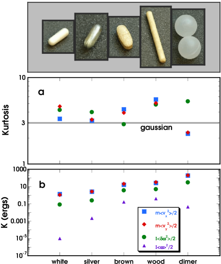
Figure 8: [AllShape] (a) Photographs of five aspherical grains; (b) the kurtosis of the speed distributions, and (c) the average kinetic energies, for the two translational and the one rotational degrees of freedom when these grains are individually fluidized. The airspeeds are 910 cm/s for the three leftmost grains, and 750 cm/s for the two rightmost grains.

A summary of the results for all grains, individually fluidized, is shown in Fig. 8. The kurtosis of the translational and rotational speed distributions is shown in the top plot. The results appear statistically greater than 3, the gaussian result, except for the translational velocity components of the dimer. The average kinetic energies are shown in the bottom plot. They too exhibit a violation of the thermal analogy since the translational kinetic energy is greater than the rotational kinetic energy. At this airspeed, the energy associated with whirling, $I\langle\omega\rangle^{2}/2$, is at least ten times smaller than the energy of angular speed fluctuations, $I\langle\delta\omega^{2}\rangle/2$. Therefore, the whirling caused by slight shape imperfections is not responsible for the breakdown of the thermal analogy.

To systematically explore the range of behavior for aspherical grains, we now vary the airflow for just one shape. We choose the silver pill, for which the thermal analogy works best in Fig. 8. Results for the average energy in each of the three kinetic degrees of freedom, $m\langle v_{x}^{2}\rangle/2$, $m\langle v_{y}^{2}\rangle/2$, and $I\langle\delta\omega^{2}\rangle/2$, as well as the whirling energy $I\langle\omega\rangle^{2}/2$, are shown in Fig. 9 along with the kurtosis of the distributions. Counter to intuition, and also counter to Eq. (2), the translational kinetic energy is nearly constant while the rotational kinetic energy actually decreases with increasing airspeed. As airspeed decreases, the kurtosis values decrease towards three and both the whirling and rotational fluctuation energies approach the translational kinetic energies. Except for the whirling, the motion is more nearly thermal at lower airspeeds.

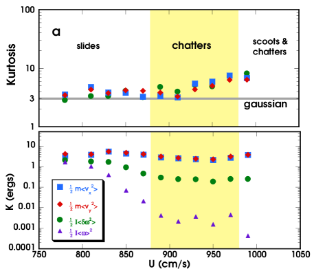
Figure 9: [Silver] (a) The kurtosis of the speed distributions, and (b) the average kinetic energies, for the two translational and the one rotational degrees of freedom for the silver grain in Fig. 8, as a function of the fluidizing airspeed.

The sequence of behavior in Fig. 9 correlates with the motion of the grain perpendicular to the sieve, which cannot be captured by our usual video methods. At low airspeeds, the grain is in physical contact with the sieve; translational motion thus requires sliding. At intermediate airspeeds, the center of mass is raised somewhat and the grain chatters back and forth along its length. This chattering becomes more prevalent as the airspeed increases. At the highest airspeeds, the chattering motion continues but with the important difference that occasionally the grain scoots rapidly across the cell. This is somewhat reminiscent of the intermittent chasing observed for two spheres of different size, and it too ruins the thermal analogy. Perpendicular motion is important for the other aspherical grains, as well. At the given airspeeds in Fig. 8, the white and silver grains both chatter steadily. The brown grain, wooden rod, and dimer all slide without chattering, like the silver grain at low airspeeds. To fully characterize and understand the behavior of aspherical grains, it would be necessary to measure their out-of-plane motion.

VII Conclusion

In summary we have explored four systematic perturbations to an experiment on nearly-levitated spheres that was previously Ojha et al. (2004, 2005) discovered to behave in perfect analogy to a thermal system. Here we find that the statistical mechanical description is robust with respect to variation of both the shape of the sample cell and with respect to the densities of the spheres. This adds to the growing list of driven out-of-equilibrium systems for which an effective temperature may be defined and used in the usual statistical mechanical sense. However, we also find that the spheres must have the same diameter or else the thermal analogy progressively breaks down as the size disparity increases. Furthermore, the analogy is well-controlled only for spherical grains. It can work for pill-shaped objects, but depends on out-of-plane motion that has not yet been well characterized. We hope that the smooth, gradual breakdown as a function of diameter ratio will stimulate theoretical work. This could lead to a better general understanding of when the concepts and tools of statistical mechanics can be invoked for driven far-from-equilibrium systems.