Two-dimensional anisotropic Heisenberg antiferromagnet in a field

Abstract

The classical, square lattice, uniaxially anisotropic Heisenberg antiferromagnet in a magnetic field parallel to the easy axis is studied using Monte Carlo techniques. The model displays a long-range ordered antiferromagnetic, an algebraically ordered spin-flop, and a paramagnetic phase. The simulations indicate that a narrow disordered phase intervenes between the ordered phases down to quite low temperatures. Results are compared to previous, partially conflicting findings on related classical models as well as the quantum variant with spin S=1/2.

I Introduction

The square lattice, uniaxially anisotropic Heisenberg antiferromagnet in an external field $H$ parallel to the easy axis has been studied since more than two decades both in its classical version lb ; gj ; kst ; cp and in the quantum variant.cu1 ; st However, important features of the phase diagram have not been definitely clarified.

The anisotropy may be introduced in various ways. In the XXZ case, the Hamiltonian may be written as

$$\mathcal{H}=J\sum\limits_{(i,j)}\left[\Delta(S_{i}^{x}S_{j}^{x}+S_{i}^{y}S_{j}^{y})+S_{i}^{z}S_{j}^{z}\right]-H\sum\limits_{i}S_{i}^{z},$$ (1)

where for the classical model $S_{i}^{x},S_{i}^{y},S_{i}^{z}$ are the components of a unit vector corresponding to the spin at site $i$ of the lattice, and the sum $(i,j)$ runs over all nearest-neighbor pairs. The coupling constant $J$ and the field $H$ are positive; the anisotropy parameter $\Delta$ may range from zero to one. The model is known to exhibit, for $0<\Delta<1$, both for simple cubic and square lattices, an antiferromagnetic (AF) phase at low temperatures and low fields, a spin-flop (SF) phase with spins canted towards the $z$-axis at larger fields, and the disordered, paramagnetic phase.

For the simple cubic lattice, the three phases are believed to meet at a bicritical point,fn belonging to the universality class of the isotropic Heisenberg model with O(3) symmetry. Elsewhere, the boundaries to the disordered phase display either Ising criticality in the AF case or XY criticality in the SF case.

For the square lattice, different scenarios on the fate of the bicritical point have been discussed following the early analysis of Landau and Binder.lb In particular, (a) the bicritical point may move to zero temperature, in accordance with the well-known theorem by Mermin and Wagner,mw with a presumably narrow disordered phase in between the AF and SF phases; (b) at low temperatures, there may be a direct transition of first order between the AF and SF phases, with a tricritical point on the boundary of the AF to the paramagnetic phase; and (c) a ’biconical phase’, in which the spins on only one of the sublattices of the antiferromagnet are canted, may intervene between the AF and SF phases at low temperatures. However, based on the early simulations lb at $\Delta=4/5$, none of these three scenarios has been strongly or even definitely favored.

More recently, related two-dimensional antiferromagnets in a field have been studied. For a classical antiferromagnet with nearest-neighbor interactions and a single-ion anisotropy, it has been suggested that the bicritical point occurs at zero temperature. However, evidence is provided by analytic approximations which are in quantitatively rather poor agreement with Monte Carlo data.cp A phase diagram with a tricritical point and a direct transition between the AF and SF phases has been determined for the quantum variant of the XXZ-model with spin $S=1/2$ and $\Delta=2/3$, see Eq. (1), corresponding to the hard-core boson Hubbard model.st For an experimentally motivated classical model mat with single-ion anisotropy and further neighbor couplings a topologically similar phase diagram has been obtained.ls

Experimentally, there seem to be quite a few quasi two-dimensional antiferromagnets with uniaxial anisotropy, including, for instance, Rb₂MnF₄, Rb₂MnCl₄, K₂MnF₄, La₅Ca₉Cu₂₄O₄₁, and Mn(HCOO)₂.mat ; gj ; exp1 ; kst ; exp2 ; exp3 ; exp4 However, the above sketched subtleties of the phase diagram have not been fully elucidated, perhaps due to additional interactions like interlayer couplings, or additional anisotropies like the breaking of the XY isotropy, which, even when being weak, are expected to affect significantly critical properties.cp Inevitable defects may eventually play an important role in two-dimensional antiferromagnets in a field being related to random-field systems.nat

In this article, we shall present results of extensive Monte Carlo simulations on the classical XXZ Heisenberg antiferromagnet on a square lattice, mostly setting the anisotropy parameter to $\Delta=4/5$ and $\Delta=2/3$. Our findings indicate that a narrow disordered phase intervenes between the AF and SF phases down to quite low temperatures.

The layout of the article is as follows. In the next section, basic properties of the model will be discussed and the quantities computed in the simulations will be listed. The transition from the SF to the paramagnetic phase will be discussed in Sec. III, followed by a section dealing with the boundary line of the AF phase. A brief discussion and summary will conclude the paper.

II Basic properties and quantities of interest

At zero temperature, $T=0$, the XXZ model on a square lattice, see Hamiltonian (1), may be easily solved exactly.lb The antiferromagnetic structure, being the ground state at low fields, becomes unstable against the spin-flop state at

$$H_{c1}=4J\sqrt{1-\Delta^{2}}.$$ (2)

Increasing the field, the paramagnetic state gets stable at $H\geq H_{c2}$, with

$$H_{c2}=4J(1+\Delta).$$ (3)

The tilt angle, $\Theta$, between the $z$-axis and the direction of the spins in the SF state, $H_{c1}\leq H\leq H_{c2}$, is given by

$$\Theta=\cos^{-1}[H/4J(1+\Delta)].$$ (4)

Obviously, in the isotropic limit, $\Delta=1$, one gets $H_{c1}=0$ and $H_{c2}=8J$, with the Ising-like AF state being squeezed out, the ground state at $H=0$ having the rotationally invariant O(3) symmetry. In the Ising limit, $\Delta=0$, one has $H_{c1}=H_{c2}=4J$, i.e. the SF structure is certainly not a ground state.

At low temperatures, considering $0<\Delta<1$, the AF and SF states give rise to ordered phases. In the AF case, one expects long-range order with the $z$-component of the sublattice magnetization as the order parameter. The transition to the paramagnetic phase is believed to be continuous and of Ising type, at least at small fields. In the SF phase, the rotational invariance of the $x$- and $y$-components of the canted spins may lead to algebraic order and a transition of Kosterlitz-Thouless type to the disordered phase,lb ; cp ; kt as it is known to hold, for instance, for the two-dimensional XY model.

Phase diagrams of the XXZ model, as obtained from our Monte Carlo simulations, are depicted in Figs. 1a and 1b. We set $\Delta=4/5$ and $\Delta=2/3$, to allow for comparison with previous findings.lb ; st The diagrams will be discussed in detail later. Unless indicated otherwise, here and in the following error bars in the figures are smaller than the size of the symbols.

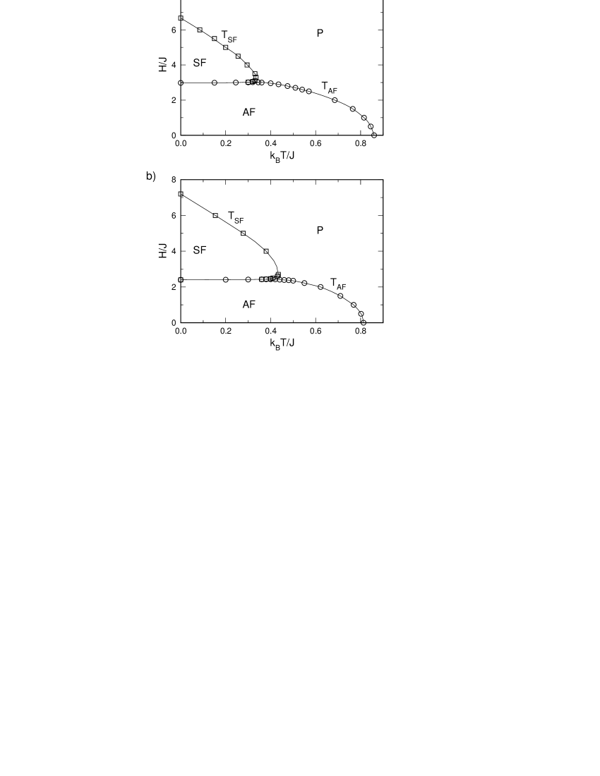
Figure 1: Simulated phase diagrams of the XXZ model on a square lattice, for the values (a) $\Delta=2/3$, and (b) $\Delta=4/5$ of the anisotropy parameter. Squares denote transitions between the SF and paramagnetic phases, circles refer to the boundary of the AF phase. Lines, here and in the following figures, are guides to the eye.

In the Monte Carlo (MC) simulations, we consider square lattices with $L\times L$ sites, employing full periodic boundary conditions. The linear dimension $L$ ranges from 2 to 240, especially to study finite-size effects allowing for extrapolation to the thermodynamic limit, $L\longrightarrow\infty$ (see below). Applying the standard Metropolis algorithm, each MC run consists of at least $10^{6}$ (and up to $10^{8}$) Monte Carlo steps per site. To obtain averages and error bars, we usually take into account several, typically about ten (and up to forty), realizations choosing various random numbers. In selected cases, especially at low temperatures close to the boundaries of the AF and SF phases, the MC runs are started with different initial configurations to check for correct equilibration.

We compute quantities of direct experimental interest as well as other quantities which enable us to conveniently determine the phase transition lines and critical properties. In particular, we calculated the specific heat $C$, both from the energy fluctuations and from the temperature derivative of the energy. Various magnetizations were computed: Especially, we recorded (i) the $z$-component of the total magnetization,

$$<M^{z}>=\Big{<}\sum\limits_{i}S_{i}^{z}\Big{>}\big{/}L^{2};$$ (5)

(ii) the square of the $z$-component of the staggered magnetization $<(M_{s}^{z})^{2}>$ (or, similarly, the absolute value) to describe the order in the antiferromagnetic phase,

$$<(M_{s}^{z})^{2}>=\Big{<}\Big{[}\sum\limits_{i_{a}}S_{i_{a}}^{z}-\sum\limits_{i_{b}}S_{i_{b}}^{z}\Big{]}^{2}\Big{>}\big{/}L^{2},$$ (6)

summing over all sites, $i_{a}$ and $i_{b}$, of the two sublattices $a$ and $b$ of the antiferromagnet; as well as (iii) the square of the staggered transverse sublattice magnetization $<(M_{s}^{xy})^{2}>$, to describe the ordering in the SF phase,

$$<(M_{s}^{xy})^{2}>\;=\;<(M_{s}^{x})^{2}>+<(M_{s}^{y})^{2}>,$$ (7)

in full analogy to Eq. (6). Alternately, one may compute the sum of the squares of each sublattice magnetization for both transverse components, as before.ls

In addition, we monitored the magnetic (staggered) susceptibility $\chi_{(s)}^{z}$, which may be obtained from the fluctuations of the (staggered) magnetization or its derivative with respect to the (staggered) field. To identify the type of transition along the boundary of the AF phase, the fourth-order, size dependent cumulant $U_{L}^{z}$ of the staggered magnetization, the Binder cumulant,bin is supposed to be rather useful:

$$U_{L}^{z}=1-<(M_{s}^{z})^{4}>_{L}\big{/}\left(3<(M_{s}^{z})^{2}>_{L}^{2}\right),$$ (8)

where $<(M_{s}^{z})^{4}>$ is defined in analogy to $<(M_{s}^{z})^{2}>$. The corresponding cumulant $U_{L}^{xy}$ may be useful to study the boundary of the SF phase. To identify the type of the phase transition, we also study the fourth-order cumulant of the energy chal

$$V_{L}=1-<E^{4}>_{L}\big{/}\left(3<E^{2}>_{L}^{2}\right),$$ (9)

with $E$ being the energy per site.

Further relevant information on the phase transitions may be inferred from histograms of the order parameter and of the energy.

III Transition from the spin-flop to the paramagnetic phase

For square lattices, the spin-flop phase has been argued to be of Kosterlitz-Thouless type,lb ; cp ; st where transverse spin correlations, i.e. $<S_{i}^{x}S_{i^{\prime}}^{x}+S_{i}^{y}S_{i^{\prime}}^{y}>$, decay algebraically with distance $|i-i^{\prime}|$ for widely separated sites $i$ and $i^{\prime}$. Closely related, the transverse sublattice magnetization $<(M_{s}^{xy})^{2}>$, see Eq. (7), describing the ordering in the SF phase, is expected to behave for $T>0$ and sufficiently large systems as

$$<(M_{s}^{xy})^{2}>_{L}\;\propto L^{-g},$$ (10)

with $g$ approaching 1/4 at the transition from the SF to the paramagnetic phase,kt ; pl and $g=2$ in the paramagnetic phase. Thence, in two dimensions, the order parameter, $<(M_{s}^{xy})^{2}>$, vanishes in the SF phase as $L\longrightarrow\infty$ at all temperatures $T>0$.

In fact, as illustrated in Fig. 2, the MC data clearly show that the magnetization decays with system size both in the SF and the paramagnetic phase. To determine the boundary of the SF phase, $T_{\text{SF}}$, from the size dependence of the transverse sublattice magnetization, Eq. (10), one may study the effective exponent, as usual,p

$$g_{\text{eff}}(L)=-\frac{\text{d}\ln<(M_{s}^{xy})^{2}>_{L}}{\text{d}\ln L},$$ (11)

in its discretized form, comparing data for consecutive system sizes, $L_{1}$ and $L_{2}$, $L_{2}>L_{1}$, with

$$g_{\text{eff}}(L_{0})=-\frac{\ln[<(M_{s}^{xy})^{2}>_{L_{2}}/<(M_{s}^{xy})^{2}>_{L_{1}}]}{\ln(L_{2}/L_{1})},$$ (12)

where $L_{0}=\sqrt{L_{1}L_{2}}$. Indeed, when crossing the phase boundary by, for instance, fixing the field and decreasing the temperature (see Figs. 1a and 1b), for large systems $g_{\text{eff}}$ tends to drop rapidly from rather high values approaching 2, characterizing the decay in the disordered phase, to a small value close to 1/4 at the transition to the SF phase. Deeper in the SF phase, $g_{\text{eff}}$ decreases somewhat to even lower values.

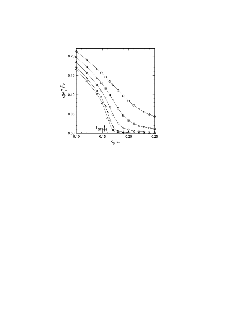
Figure 2: Square of the staggered transverse sublattice magnetization, $<(M_{s}^{xy})^{2}>_{L}$, vs. temperature at fixed field $H/J=6.0$ for systems of size $L=10$, 20, 40, 80, and 120 (from top to bottom), close to the boundary between spin-flop and disordered phases. The anisotropy parameter is $\Delta=4/5$.

This behavior of the effective exponent is exemplified in Fig. 3, allowing one to estimate $T_{\text{SF}}$. We checked the approach by analyzing the two-dimensional (planar) XY model, reproducing quite accurately the transition temperature as obtained from elaborate numerical studies.b

The Kosterlitz-Thouless character of the transition between the SF and the paramagnetic phases is also reflected in the thermal behavior of the specific heat $C$, which displays a non-critical maximum close to, but not exactly at the transition. Of course, from simulational data one cannot identify the expected essential singularity of $C$ at the transition.

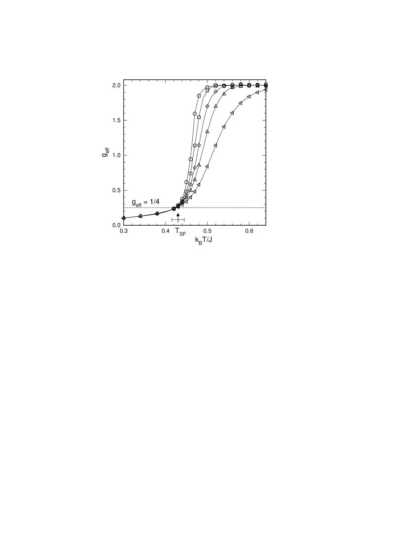
Figure 3: Effective exponent $g_{\text{eff}}$, see Eqs. (11) and (12), vs. temperature at fixed field $H/J=2.7$, comparing systems of size $(L_{2},L_{1})$= (20,10), (30,20), (40,30), (60,40), and (80,60) (from bottom to top), close to the boundary between spin-flop and disordered phases. The anisotropy parameter is $\Delta=4/5$.

Approximate analytic expressions for the boundary between the SF and the paramagnetic phases may be obtained by the following considerations, slightly modifying previous arguments.lb Using polar coordinates and fixing the $z$-component of the spins in the SF phase to its value in the ground state, Eq. (4), the transition temperature $T_{\text{SF}}$ may be approximated by lb

$$\frac{k_{B}T_{\text{SF}}}{J}=\frac{k_{B}T_{\text{KT}}}{J}\,\Delta\left[1-(H/H_{c2})^{2}\right],$$ (13)

where $k_{B}T_{\text{KT}}/J$ refers to the Kosterlitz-Thouless transition temperature of the XY model with coupling $J$, i.e. the classical isotropic model with a two-component spin vector of length one.b Indeed, this approximate expression may be regarded as an upper bound to the true transition temperature, because the fluctuations in the $z$-component (which, in turn, are coupled to the fluctuations in the transverse spin components) tend to reduce the transition temperature. In addition, the change of the tilt angle $\Theta$ with temperature, at fixed field, will affect the transition temperature. In fact, $T_{\text{SF}}$, as determined in the simulations, see Figs. 1a and 1b, is seen to be lower than suggested by Eq. (13). In any event, the approximation does not hold in the vicinity of $H_{c1}$, where the fluctuations of the longitudinal and transverse spin components are strongly correlated. Among others, that region will be discussed in the next section.

IV The boundary line of the antiferromagnetic phase

We determined the boundary line of the AF phase by monitoring especially the specific heat $C$, the square of the $z$-component of the staggered magnetization, $<(M_{s}^{z})^{2}>$, the staggered susceptibility, $\chi_{s}^{z}$, and the Binder cumulant, $U_{L}^{z}$. The transition temperatures follow from finite-size extrapolations of the Monte Carlo data. Results for $\Delta=4/5$ and $\Delta=2/3$ are displayed in Fig. 1.

At low fields and high temperatures the transition is expected to be continuous and of Ising type. Indeed, we observe, for instance, a logarithmic divergence in the height of the peak in the specific heat as a function of system size, $C_{\text{max}}\propto\ln L$, and an effective critical exponent of the order parameter $\beta_{\text{eff}}$ consistent with the asymptotic value 1/8 when approaching the transition, fixing the field and varying temperature.

The transition line of the AF phase shows a maximum in the critical field, as a function of temperature, being somewhat higher than $H_{c1}$, Eq. (2), both for $\Delta=2/3$ and $\Delta=4/5$ (a feature which has not been mentioned in the early worklb ). In that part of the phase diagram, see Fig. 4 for $\Delta=4/5$, the boundary lines of the SF and AF phases approach each other, when lowering the temperature.

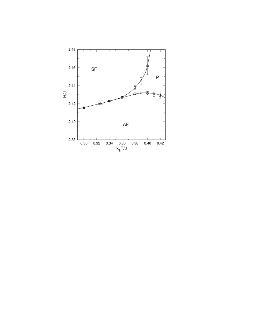
Figure 4: Details of the phase diagram of the XXZ model on a square lattice with $\Delta=4/5$. Squares refer to the boundary of the SF, circles to that of the AF phase.

Fixing the field to be slightly below its maximal critical value and decreasing the temperature, one observes a rather asymmetric behavior in the staggered magnetization $<(M_{s}^{z})^{2}>$, as illustrated in Fig. 5. The order parameter of the AF phase rises fairly gradually entering the AF phase from the paramagnetic phase, while it drops down rather rapidly on approach to the SF phase. This asymmetry signals either a change in the type of the transition at the lower temperature, becoming, possibly, of first order, or in the extent of the critical region becoming, possibly, very narrow.

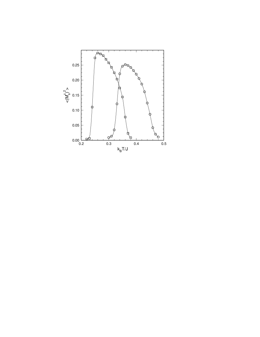
Figure 5: Staggered magnetization $<(M_{s}^{z})^{2}>$ vs. temperature at field $H/J=3.0$ for $\Delta=2/3$ with $L=128$ (squares), and at $H/J$= 2.42 for $\Delta=4/5$ with $L=120$ (circles), close to the maximum of the boundary of the AF phase.

To study the transition along the boundary of the AF phase in more detail, the Binder cumulant $U_{L}^{z}$ may be quite useful, as had been employed before.st ; ls In the thermodynamic limit the value of the cumulant at the transition point, the critical cumulant $U_{L=\infty}^{z}(T_{\text{AF}})$, is believed to characterize the type and universality class of the transition. From simulational data, the critical cumulant may be estimated from the intersection value $U^{I}(L)$ of the cumulant for different system sizes $L$ and $L^{\prime}=bL$ (in the following, we set $b=2$), doing finite-size extrapolations.bin In Fig. 6, we depict results for $\Delta=4/5$, monitoring $U^{I}(L)$ as a function of temperature in the vicinity of the AF boundary line. The intersection value $U^{I}$ seems to display one plateau at higher temperatures and another plateau, with a smaller height, at lower temperatures, with a fairly rapid change in between. The plateaus tend to get more pronounced and the change becomes sharper as the system size $L$ is increased. In fact, the plateau at high temperatures is obviously related to the critical cumulant in the universality class of the two-dimensional Ising model, where $U_{L=\infty}(T_{\text{AF}})\approx 0.6106$.bn Note that $U_{L}^{z}$, computed exactly at the transition $(T_{\text{AF}},H_{\text{AF}})$, approaches this value closely with only minor finite-size corrections for low fields and high temperatures. However, near the maximum of the boundary line of the AF phase, significant corrections are observed, which have not been discussed in the related quantum variant.st The critical cumulant of the apparent plateau at low temperatures tends to increase weakly with T, being close to 0.4 at $\Delta=4/5$, for the system sizes we considered, $L\leq 120$. Perhaps interestingly, at the critical field $H_{c1}(\Delta)$, the cumulant seems to approach, at least for small lattices, in the limit $T\longrightarrow 0$, a value close to 0.38. With decreasing $\Delta$, this limiting value decreases.

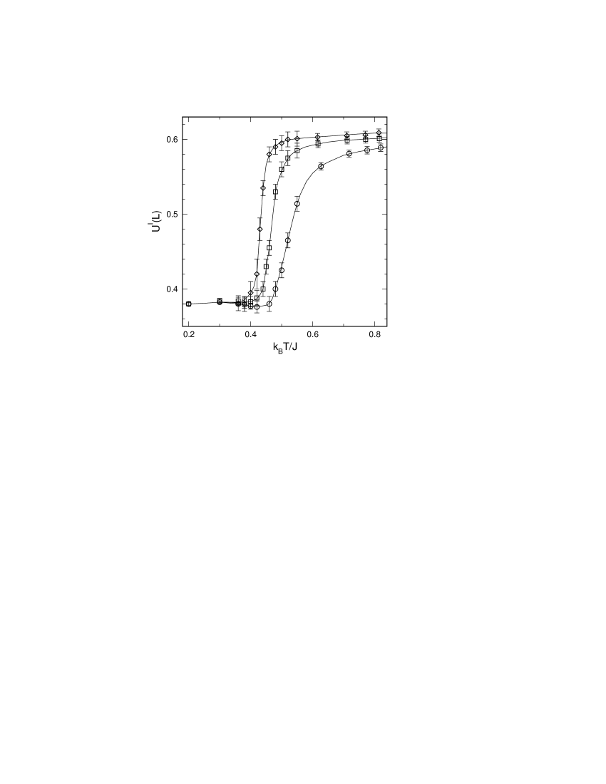
Figure 6: Binder cumulant $U^{I}(L)$, as obtained from the intersection points of cumulants for lattices of sizes $L$ and $2L$ close to the boundary of the AF phase, as a function of temperature, with $L$= 10, 20, and 40 (from bottom to top). The anisotropy parameter is $\Delta=4/5$.

Note that the turning point of the intersection value $U^{I}(L)$ is shifted towards lower temperatures, $T_{\text{tu}}$, as $L$ increases, see Figs. 6 and 7. Obviously, there are uncertainties in extrapolating those data to the thermodynamic limit. A naive linear extrapolation yields an estimate of a temperature, $T^{*}$, of about 0.4 (in units of $J/k_{B}$), at which non-Ising criticality may set in, possibly due to a transition of first order.

Figure 7: Size dependence of the turning point, $T_{\text{tu}}$, in the Binder cumulant $U^{I}(L)$ comparing lattices of linear dimension $L$ and $2L$, for $\Delta=4/5$, see Fig. 6, with $L$ ranging from 4 to 60.

This interpretation, however, has to be viewed with much care. Indeed, the fourth order energy cumulant chal gives no hint of a transition of first order at the AF boundary, at quite low temperatures, $0.3J/k_{B}\leq T<T^{*}$. Its minimum near the transition, becoming even more shallow at lower temperatures, tends to vanish for larger lattices, as expected for a continuous transition.

Even more strikingly, the size dependences of the specific heat as well as of the staggered susceptibility suggest that the boundary line of the AF phase is still in the Ising universality class well below the anticipated change at $T^{*}$. This behavior is exemplified in Figs. 8 and 9 for the case $\Delta=4/5$ and $H/J=2.42$, where $k_{B}T_{\text{AF}}/J\approx 0.33$, i.e. in the part of the phase diagram where the AF and SF phase boundaries are hardly discernible, see Fig. 4. We find consistency with Ising criticality, especially, $C_{\text{max}}\propto\ln L$, and the peak of the staggered susceptibility, $(\chi_{s}^{z})_{\text{max}}$, grows like $L^{\gamma/\nu}=L^{7/4}$. We checked equilibration of the MC data by monitoring time series of the energy and the staggered magnetization as well as by calculating the specific heat from the energy fluctuations and the temperature derivative of the energy. The findings suggest that there is a very narrow paramagnetic phase intervening between the AF and SF phases at least down to that temperature, $k_{B}T/J\approx 0.33$. At even lower temperatures, this type of analysis would require very large computational resources to obtain reliable MC data.

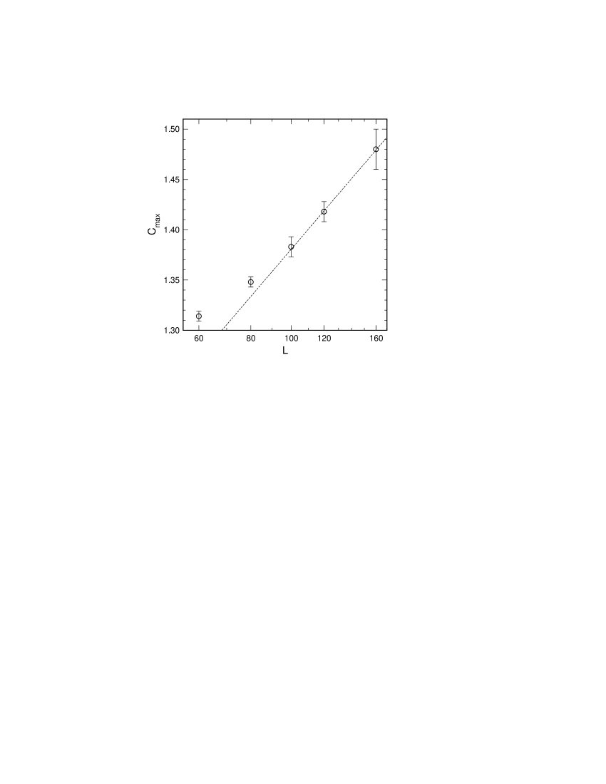
Figure 8: Maximum in the specific heat vs. logarithm of the system size $L$ at $H/J=2.42$ and $\Delta=4/5$ at temperatures close to $k_{B}T_{\text{AF}}/J\approx 0.33$, see Fig. 4. The dashed line indicates a logarithmic size dependence.

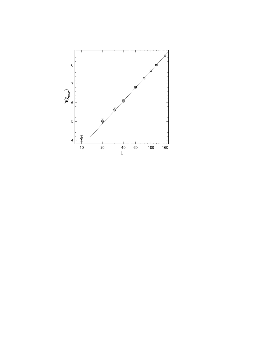
Figure 9: Doubly logarithmic plot of the size dependence of the maximum in the staggered susceptibility at $H/J=2.42$ and $\Delta=4/5$. The dashed line refers to a slope with $\gamma/\nu=7/4$.

For $\Delta=2/3$, similar features are observed in the corresponding part of the phase diagram, where, e.g., a logarithmic size dependence of the height of the specific heat at temperatures close to $k_{B}T_{\text{AF}}/J\approx 0.28$ is found, compare Fig. 1.

In contrast, results of our simulations of the XXZ model on a simple cubic lattice, setting $\Delta=4/5$, show at temperatures below the bicritical point a direct transition of first order between the AF and SF phases, as expected.fn ; bl2 For instance, the maximum of the specific heat increases with a power law in $L$, with an effective exponent, for moderate system sizes, $8\leq L\leq 20$, being significantly larger than the value characteristic for the universality class of the three-dimensional Ising model. The behavior is, indeed, indicative of a first order transition, where $C_{\text{max}}\propto L^{3}$. Likewise, energy histograms show the usual properties of a transition of first order, with an overlap of two distinct Gaussian peaks. The critical energy cumulant in the three-dimensional case is observed to be close to, but distinct from 2/3.

Note that at fixed low temperature and varying the field, the $z$-component of the magnetization changes rapidly in both sublattices simultaneously, within our field resolution, both for $\Delta=4/5$ and $\Delta=2/3$, contradicting a biconical intermediate phase with a canting of the spins in only one sublattice.

V Discussion and summary

We have studied the classical, square lattice, uniaxially anisotropic Heisenberg antiferromagnet, the XXZ model, in a magnetic field, doing extensive Monte Carlo simulations. We mainly considered two cases of fairly weak anisotropy, $\Delta=4/5$ and $\Delta=2/3$.

The model displays an antiferromagnetic, a spin-flop, and a paramagnetic phase.

The transition from the antiferromagnetic to the paramagnetic phase is seen to be of Ising type at small fields, remaining of that type at higher fields and rather low temperatures (down to at least $k_{B}T/J\approx 0.33$ in the case $\Delta=4/5$), as inferred, especially, from the size dependence of the maxima in the staggered susceptibility and the specific heat. A naive analysis of MC data of the Binder cumulant along the boundary of the antiferromagnetic phase may lead to a different, but supposedly erroneous conclusion. Presumably, the critical region at the AF phase boundary becomes rather tiny when the SF and AF phase boundaries approach each other, demanding very large lattices to identify the universality class correctly, at least when studying the Binder cumulant.

The transition between the spin-flop and the disordered phase is of Kosterlitz-Thouless type. It may be located accurately by analyzing the finite-size behavior of the transverse staggered magnetization, vanishing with increasing system size with a characteristic power law at the transition.

In the quantum variant of the model with spin $S=1/2$ a tricritical point on the AF boundary and a direct transition between the AF and SF phases at low temperatures have been obtained.st Near the tricritical point the AF and SF phases are still well separated. At present, we can only speculate whether this, perhaps, surprising discrepancy between the classical and quantum models could be resolved when the classical version would be analyzed at even lower temperatures or when MC data on the quantum version would be reanalyzed.

In the isotropic limit, $\Delta=1$, one finds, in non-vanishing field, $H>0$, a spin-flop phase of Kosterlitz-Thouless character both in the classical and in the quantum model.lb ; cu2 For $\Delta<1$ and $H=0$, an Ising type transition occurs at a non-zero temperature, with the transition temperature moving to zero as the anisotropy vanishes, $\Delta\longrightarrow 1$, again both in the classical and the quantum case.bar ; cu1

One of the remaining open crucial questions is, whether there is a typical phase diagram for square lattice, uniaxially anisotropic antiferromagnets. In the case of the antiferromagnetic nearest-neighbor Heisenberg model with single-ion anisotropy, a phase diagram with a paramagnetic phase between the antiferromagnetic and spin-flop phases extending down to arbitrarily low temperatures has been suggested.cp In another study of that model, a conflicting scenario with a direct transition between the AF and SF phases has been favored, presenting, however, only few Monte Carlo data.kst Including more than nearest-neighbor interactions in an antiferromagnet with single-ion anisotropy,mat ; ls or taking into account quantum fluctuations,st phase diagrams with a tricritical point and a direct transition between the AF and SF phases have been obtained.

In any event, we should like to encourage future work on this and related models, which may also serve as a guide in interpreting experiments on corresponding quasi two-dimensional anisotropic antiferromagnets.

- (1) D. P. Landau and K. Binder, Phys. Rev. B 24, 1391 (1981).
- (2) H. J. M. de Groot and L. J. de Jongh, Physica B 141, 1 (1986).
- (3) R. van de Kamp, M. Steiner, and H. Tietze–Jaensch, Physica B 241, 570 (1997).
- (4) B. V. Costa and A. S. T. Pires, J. Magn. Magn. Mat. 262, 316 (2003).
- (5) A. Cuccoli, T. Roscilde, V. Tognetti, R. Vaia, and P. Verrucchi, Phys. Rev. B 67, 104414 (2003).
- (6) G. Schmid, S. Todo, M. Troyer, and A. Dorneich, Phys. Rev. Lett. 88, 167208 (2002).
- (7) M. E. Fisher and D. R. Nelson, Phys. Rev. Lett. 32, 1350 (1974).
- (8) M. E. Mermin and H. Wagner, Phys. Rev. Lett. 17, 1133 (1966); 17, 1307 (1966).
- (9) M. Matsuda, K. Kakurai, J. E. Lorenzo, L. P. Regnault, A. Hiess, and G. Shirane, Phys. Rev. B 68, 060406(R) (2003).
- (10) R. Leidl and W. Selke, Phys. Rev. B 69, 056401 (2004); Phys. Rev. B 70, 174425 (2004).
- (11) H. Rauh, W. A. C. Erkelens, L. P. Regnault, J. Rossat–Mignod, W. Kullmann, and R. Geick, J. Phys. C 19, 4503 (1986).
- (12) R. A. Cowley, A. Aharony, R. J. Birgeneau, R. A. Pelcovits, G. Shirane, and T. R. Thurston, Z. Phys. B 93, 5 (1993).
- (13) R. J. Christianson, R. L. Leheny, R. J. Birgeneau, and R. W. Erwin, Phys. Rev. B 63, 140401(R) (2001).
- (14) U. Ammerahl, B. Büchner, C. Kerpen, R. Gross, and A. Revcolevschi, Phys. Rev. B 62, R3592 (2000); R. Klingeler, Ph.D. thesis, RWTH Aachen (2003).
- (15) T. Nattermann and J. Villain, Phase Transitions 11, 5 (1988).
- (16) J. M. Kosterlitz and D. J. Thouless, J. Phys. C 6, 1181 (1973).
- (17) K. Binder, Z. Phys. B 43, 119 (1981).
- (18) M. S. S. Challa, D. P. Landau, and K. Binder, Phys. Rev. B 34, 1841 (1986).
- (19) P. Peczak and D. P. Landau, Phys. Rev. B 43, 1048 (1991).
- (20) M. Pleimling and W. Selke, Eur. Phys. J. B 1, 385 (1998).
- (21) B. Berche, J. Phys. A 36, 585 (2003); R. Gupta and C. F. Baillie, Phys. Rev. B 45, 2883 (1992).
- (22) G. Kamieniarz and H. W. J. Blöte, J. Phys. A 26, 201 (1993); D. Nicolaides and A. D. Bruce, J. Phys. A 21, 233 (1988).
- (23) D. P. Landau and K. Binder, Phys. Rev. B 17, 2328 (1978).
- (24) A. Cuccoli, T. Roscilde, R. Vaia, and P. Verrucchi, Phys. Rev. B 68, 060402(R) (2003).
- (25) T. Barnes, K. J. Cappon, E. Dagotto, D. Kotchan, and E. S. Swanson, Phys. Rev. B 40, 8945 (1989).