Circuit theory for noise in incoherent normal–superconducting dot structures

Abstract

We consider the current fluctuations in a mesoscopic circuit consisting of nodes connected by arbitrary connectors, in a setup with multiple normal or superconducting terminals. In the limit of weak superconducting proximity effect, simplified equations for the second-order cross-correlators can be derived from the general counting field theory, and the result coincides with the semiclassical principle of minimal correlations. We discuss the derivation of this result in a multi-dot case.

Fluctuations of charge current in mesoscopic structures are in general sensitive to the interactions and the fermionic nature of electrons. In multi-terminal setups, the geometry of the circuit is important for the cross-correlations, and in superconducting heterostructures, also the Andreev reflection, the superconducting proximity effect and transmission properties of NS interfaces need to be accounted for.

The general theory for the full counting statistics of current fluctuations in multi-terminal structures was outlined in Ref. Yu. V. Nazarov and Bagrets, 2002. The calculation of the second-order correlators using this theory can be simplified, from complicated $4\times 4$ matrix equations to a Kirchoff-type system for scalar parameters, using an approach discussed also, for example, in Refs. Samuelsson and Büttiker, 2002a; Nagaev et al., 2002. In the incoherent case, Nagaev and Büttiker (2001); Samuelsson and Büttiker (2002a); Belzig and Samuelsson (2003) the result coincides with the semiclassical principle of minimal correlations. Samuelsson and Büttiker (2002a); Nagaev et al. (2002) In this paper we show the derivation of this result in a multi-dot system, and consider a few special cases.

The theory considers a network of normal ($\mathcal{T}_{N}$) and superconducting ($\mathcal{T}_{S}$) terminals ($\mathcal{T}=\mathcal{T}_{N}\cup\mathcal{T}_{S}$) and nodes ($\mathcal{N}$), connected by connectors. Each connector $(i,j)$ is described by its transmission eigenvalues $T_{n}^{ij}$, Blanter and Büttiker (2000) and each node $j$ is characterized by a Keldysh Green function $\check{G}_{j}$, which is a $4\times 4$ matrix in the Keldysh($\check{~{}}$) $\,\otimes\,$ Nambu($\hat{~{}}$) space. In the quasiclassical approximation, assuming stationary state and isotropicity, these are only functions of energy, $\check{G}(\varepsilon)$.

The statistics of the current in the circuit is connected to the generating function $S(\{\chi_{k}\}_{k\in\mathcal{T}})$ of charge transfer, which can be found by solving transport equations for the Green functions. In the stationary case at zero frequency, the noise correlations $\tilde{S}_{kl}$ between the fluctuations $\delta I_{k}=I_{k}-\left<{I_{k}}\right>$ of currents flowing into the terminals $k,l\in\mathcal{T}$ relate to it through Yu. V. Nazarov and Bagrets (2002); Belzig (2003)

$$\tilde{S}_{kl}\equiv\int_{-\infty}^{\infty}\!\frac{\text{d}t}{2}\left<{\left\{\delta I_{k}(t),\delta I_{l}(0)\right\}}\right>=-\frac{e^{2}}{t_{0}}\left.\frac{\partial^{2}S}{\partial\chi_{k}\partial\chi_{l}}\right|_{\{\chi_{j}\}=0}\,.$$ (1)

Here, $t_{0}$ is the duration of the measurement, and the equality applies provided this is much larger than the correlation time of the fluctuations.

The boundary conditions for transport are assumed such that the terminals are in an internal equilibrium, where the Green function has the form

$$\check{G}_{\text{eq}}=\begin{pmatrix}\hat{R}&\hat{K}\\ \hat{0}&\hat{A}\end{pmatrix},\;\begin{aligned} \hat{R}&=u\hat{\tau}_{3}+vi\hat{\tau}_{2}\,,\;\hat{K}=\hat{R}\hat{h}-\hat{h}\hat{A}\,,\\ \hat{A}&=-\hat{\tau}_{3}\hat{R}^{\dagger}\hat{\tau}_{3}\,,\;\hat{h}=f_{L}+\hat{\tau}_{3}f_{T}\,.\end{aligned}$$ (2)

Here, $u=\left\lvert{\varepsilon}\right\rvert/\sqrt{\varepsilon^{2}-\Delta^{2}}$, $v=\operatorname{sgn}(\varepsilon)\sqrt{u^{2}-1}$ are the coherence factors, and $\Delta$ is the superconducting pair amplitude. The functions $f_{T}(\varepsilon)=1-f_{0}(-\varepsilon)-f_{0}(\varepsilon)$ and $f_{L}(\varepsilon)=f_{0}(-\varepsilon)-f_{0}(\varepsilon)$ are the symmetric and antisymmetric parts of $f_{0}(\varepsilon)=[e^{(\varepsilon-eV)/(k_{B}T)}+1]^{-1}$, where $T$ is the temperature and $V$ the potential of the terminal. We assume $V=0$ in all S terminals to avoid time-dependent effects. For calculation of the statistics of the current, the counting field theory additionally specifies the rotation

$$\check{G}_{k}(\chi_{k})=e^{i\chi_{k}\check{\tau}_{K}/2}\;\check{G}_{k,\text{eq}}\;e^{-i\chi\check{\tau}_{K}/2}\,,\quad\check{\tau}_{K}\equiv\check{\tau}_{1}\otimes\hat{\tau}_{3}\,,$$ (3)

at each terminal $k$, which connects the “counting fields” $\chi_{k}$ to the Green functions.

In circuit theory, Yu. V. Nazarov (1999) transport is modeled by the conservation of the matrix current at each node $i$

$$\sum_{j\in\mathcal{C}}\check{I}^{ij}=\check{0}\,,\;\check{I}^{ij}=\frac{2e^{2}}{\pi\hbar}\sum_{n}\frac{T_{n}^{ij}\left[\check{G}_{j},\check{G}_{i}\right]}{4+T_{n}^{ij}\bigl{(}\left\{\check{G}_{i},\check{G}_{j}\right\}-2\bigr{)}}\,.$$ (4)

The sum runs over all nodes and terminals ($\mathcal{C}=\mathcal{T}\cup\mathcal{N}$): we assume the convention that $T_{n}^{ij}=0$ for $i=j$ and disconnected points. This matrix is related to the observable charge and energy currents by

$$I^{ij}=\frac{1}{8e}\int_{{-\infty}}^{\infty}\mathrm{d}\varepsilon\;\text{Tr}\left[\check{\tau}_{K}\check{I}^{ij}\right]\,,\;I_{E}^{ij}=\frac{1}{8e^{2}}\int_{{-\infty}}^{\infty}\mathrm{d}\varepsilon\;\varepsilon\text{Tr}\left[\check{\tau}_{1}\check{I}^{ij}\right]\,.$$ (5)

Their dependency on $\{\chi_{i}\}$, in turn, describes the generating function of charge transfer: Yu. V. Nazarov and Bagrets (2002)

$$\mathrm{d}S(\{\chi_{l}\})=-\frac{t_{0}}{e}\sum_{k\in\mathcal{T}}\sum_{j\in\mathcal{C}}I^{jk}(\{\chi_{l}\})\;\,\mathrm{d}(i\chi_{k})\,.$$ (6)

Determining the Green functions at the nodes from Eqs. (3,4) and finally applying Eqs. (5,6), one can in principle find the distribution of the fluctuations in the current. However, the problem becomes considerably simpler if one is interested only in the second moment of this distribution, i.e., the current noise as given in Eq. (1).

We proceed calculating the noise by assuming that the superconducting proximity effect is negligible, so that the anomalous parts ($\propto\hat{\tau}_{1},\hat{\tau}_{2})$ of the functions vanish in each node. Samuelsson and Büttiker (2002a); Belzig and Samuelsson (2003) Then, one can expand the Green function at node $j$ to the first order in the counting fields $\{\chi_{k}\}$, in the Nambu-diagonal form: Samuelsson and Büttiker (2002a); Nagaev et al. (2002); Houzet and Pistolesi (2004)

$$\check{G}_{j}=\begin{pmatrix}\hat{\tau}_{3}&2\hat{h}_{j}\hat{\tau}_{3}\\ 0&-\hat{\tau}_{3}\end{pmatrix}+\sum_{k\in\mathcal{T}}i\chi_{k}\begin{pmatrix}-\hat{h}_{j}\hat{b}^{j}_{k}&4\hat{c}^{j}_{k}-\hat{b}^{j}_{k}\\ \hat{b}^{j}_{k}&\hat{h}_{j}\hat{b}^{j}_{k}\end{pmatrix}+\ldots,$$ (7)

where $\hat{b}_{k}^{j}(\varepsilon)=\hat{1}b_{k}^{j}(\left\lvert{\varepsilon}\right\rvert)$, $\hat{c}_{k}^{j}=c_{T}^{jk}+\hat{\tau}_{3}c_{L}^{jk}$ and $\hat{h}=f_{L}+\hat{\tau}_{3}f_{T}$. This satisfies the quasiclassical normalization $\check{G}_{j}^{2}=\check{1}$ up to second order in $\{\chi_{k}\}$. For the matrix currents, the above corresponds to the expansion

$$\check{I}^{ij}=\begin{pmatrix}\hat{0}&\hat{I}_{0}^{ij}\\ \hat{0}&\hat{0}\end{pmatrix}+\sum_{k\in\mathcal{T}}i\chi_{k}\begin{pmatrix}\hat{0}&\hat{I}_{c,k}^{ij}-\hat{I}_{b,k}^{ij}\\ \hat{I}_{b,k}^{ij}&\hat{0}\end{pmatrix}+\ldots+\check{I}_{\text{coh.}}^{ij}$$ (8)

of Eq. (4), where $\hat{I}_{0}$, $\hat{I}_{b,k}$ and $\hat{I}_{c,k}$ have the structure $\hat{I}=\hat{\tau}_{3}I(\hat{\tau}_{3}\varepsilon)$, due to symmetries in the Nambu space. Here, $\check{I}_{\text{coh.}}(\{\chi_{k}\})$ contains the off-diagonal Nambu-elements, present if $j$ corresponds to a superconducting terminal. In what follows, we neglect this coherent part of the current, assuming there are additional decoherence-inducing sink terms in Eq. (4). Samuelsson and Büttiker (2002a); Belzig and Samuelsson (2003) This is valid provided that the Thouless energy describing the inverse time of flight through the node or the connector is much less than the characteristic energy scales of the problem, or, if there is a strong pair-breaking effect in the node, e.g., due to magnetic impurities.

One can then consider expansion (8) in detail, assuming a node $i$ is connected to a node or terminal $j$. This yields four independent equations of conservation:

$$\sum_{j\in\mathcal{C}}I_{T}^{ij}=0,\;\sum_{j\in\mathcal{C}}I_{L}^{ij}=0,\;\sum_{j\in\mathcal{C}}I_{b,k}^{ij}=0,\;\sum_{j\in\mathcal{C}}I_{c,T,k}^{ij}=0\,,$$ (9)

in which $I_{T}$ corresponds to the spectral charge current, $I_{L}$ to the energy current, and the last two to a “noise” current, with the symmetric part defined as $I_{c,T,k}(\varepsilon)=I_{c,k}(\varepsilon)+I_{c,k}(-\varepsilon)$. The corresponding antisymmetric current $I_{c,L,k}^{ij}$ is not needed, as we concentrate on the noise in the charge current. The spectral currents have the form

$$I_{T}^{ij}=g_{ij}(f_{T}^{j}-f_{T}^{i})\,,\quad I_{b,k}^{ij}=g_{ij}(b^{j}_{k}-b_{k}^{i})\,,$$ (10a)

$$I_{L}^{ij}=\begin{cases}0&\text{for $j\in\mathcal{T}_{S}$ and $\left\lvert{\varepsilon}\right\rvert<\left\lvert{\Delta}\right\rvert$,}\\ g_{ij}(f_{L}^{j}-f_{L}^{i})&\text{otherwise.}\end{cases}$$ (10b)

Thus, no energy current flows to the superconductors for $\left\lvert{\varepsilon}\right\rvert<\left\lvert{\Delta}\right\rvert$. The fourth current is

$$\frac{1}{4}I_{c,T,k}^{ij}=g_{ij}(c_{T}^{ik}-c_{T}^{jk})-(b_{k}^{i}-b_{k}^{j})(s_{ij}(\varepsilon)+s_{ij}(-\varepsilon))\,,$$ (11)

but it can be eliminated, see below.

The factors $g_{ij}$ and $s_{ij}(\varepsilon)$ appearing in the expansion can be identified as the conductances and spectral noise densities characteristic of the connectors, and their exact form depends on whether the connector lies between two normal points (NN) or between a normal and a superconducting point (NS). The expressions for the NS case are lengthy, so for simplicity we use here only the limits $\varepsilon\ll\Delta$ and $\varepsilon\gg\Delta$ for superconducting Green’s functions, effectively neglecting the exact form of the superconducting density of states (DOS). In this approximation, for an NS connector at $\left\lvert{\varepsilon}\right\rvert\gg\left\lvert{\Delta}\right\rvert$ or an NN connector,

$$\begin{split}s_{ij}^{NN}(\varepsilon)=\frac{1}{4}g_{ij}^{NN}[&2-(f_{L}^{i}+f_{T}^{i})^{2}-(f_{L}^{j}+f_{T}^{j})^{2}\\ &+F_{ij}^{NN}(f_{L}^{i}+f_{T}^{i}-f_{L}^{j}-f_{T}^{j})^{2}]\,,\end{split}$$ (12a)

$$g_{ij}^{NN}=\frac{e^{2}}{\pi\hbar}\sum_{n}T_{n}^{ij}\,,\;F_{ij}^{NN}=\frac{e^{2}}{g_{ij}^{NN}\pi\hbar}\sum_{n}T_{n}^{ij}(1-T_{n}^{ij})\,.$$ (12b)

The result for an NS connector at $\left\lvert{\varepsilon}\right\rvert\ll\left\lvert{\Delta}\right\rvert$ is

$$s_{ij}^{NS}(\varepsilon)=\frac{1}{2}g_{ij}^{NS}[1-(f_{L}^{i})^{2}-(f_{T}^{i})^{2}+F_{ij}^{NS}(f_{T}^{i})^{2}]\,,$$ (13a)

$$g_{ij}^{NS}=\frac{e^{2}}{\pi\hbar}\sum_{n}\frac{2(T_{n}^{ij})^{2}}{(2-T_{n}^{ij})^{2}}\,,$$ (13b)

$$F_{ij}^{NS}=\bigl{(}g_{ij}^{NS}\bigr{)}^{-1}\,\frac{e^{2}}{\pi\hbar}\sum_{n}\frac{16(T_{n}^{ij})^{2}}{(2-T_{n}^{ij})^{4}}(1-T_{n}^{ij})\,,$$ (13c)

as found through an expansion of Eq. (4). Naturally, the results above agree with expressions for the noise generated between two terminals, with $F_{ij}$ being the differential Fano factor. Blanter and Büttiker (2000); de Jong and Beenakker (1994)

The above equations are supplied with the boundary conditions

$$b_{k}^{l}=\delta_{kl}\,,\quad c_{k}^{l}=0\,,\quad f_{k}(\varepsilon)=f_{0}(\varepsilon,V_{k},T_{k})\,,$$ (14)

where $k$ and $l$ are indices of terminals. These can be found by comparing expansion (7) to Eq. (3) (for N terminals), and by examining the expression for $\check{I}$ (for S terminals).

Finally, Eqs. (1,5,6) yield the result

$$\tilde{S}_{kl} =\sum_{j\in\mathcal{C}}\int_{{-\infty}}^{\infty}\mathrm{d}\varepsilon\;\frac{1}{8}I_{c,T,l}^{kj}$$

$$=\sum_{(i,j)}\int_{{-\infty}}^{\infty}\mathrm{d}\varepsilon\;(b_{k}^{i}-b_{k}^{j})(b_{l}^{i}-b_{l}^{j})s_{ij}(\varepsilon)\,,\,$$ (15)

for the correlations between terminals $k$ and $l$. In the last step, we eliminated all $c_{T,k}^{i}$ from the set of equations, which transforms the result to a sum over all connectors $(i,j)$ in the circuit.

The equations above have a simple physical interpretation. The first two of Eqs. (9) describe the conservation of charge (T) and energy (L) currents at each energy interval $[\varepsilon,\varepsilon+\mathrm{d}\varepsilon]$. With boundary conditions (14,12,13), they yield distribution functions $f_{L}^{i}$, $f_{T}^{i}$ of electrons at the nodes. In addition, one needs to solve from Eqs. (9) the variable $b_{k}^{i}$, which characterizes the coupling between terminal $k$ and node $i$. It turns out that this quantity is in fact the characteristic potential introduced for semiclassical multiterminal calculations. Büttiker (1993) Knowing $f$, the standard two-terminal relations Beenakker (1997) (12,13) give the spectral noise densities in each connector, and Eq. (15) describes how these couple to the terminals. The final result is similar to the semiclassical result in diffusive metals, Sukhorukov and Loss (1998) and coincides with the result in dot systems, see below.

The assumption of all nodes being in the normal state resulted in a simple way to handle superconductors in one special case: first, it takes into account that no energy current enters superconductors at $\left\lvert{\varepsilon}\right\rvert<\left\lvert{\Delta}\right\rvert$, and second, assumes that other effects due to superconductivity are localized in only one connector, where both the conductivity and the generated noise are modified. Our last approximation of a piecewise constant superconducting DOS simplifies the resulting expressions.

We implicitly assumed above that there is no inelastic scattering which would drive the system towards equilibrium. However, following Ref. Nagaev, 1995, a strong relaxation of the distribution function in a node may be modeled by assuming that $f_{j}$ has the form of a Fermi function. In the case of relaxation due to strong electron-electron scattering, the corresponding potential $V_{j}$ and temperature $T_{j}$ can be determined by taking the two first moments, $\int\text{d}\varepsilon$ and $\int\text{d}\varepsilon\varepsilon$ of Eqs. (9):

$$\sum_{j\in\mathcal{C}}g_{ij}(V_{i}-V_{j})=0\,,\quad\mathcal{L}^{-1}\equiv\frac{3e^{2}}{k_{B}^{2}\pi^{2}}\,,$$ (16a)

$$\sum_{j\in\mathcal{C}\setminus\mathcal{T}_{S}}g_{ij}[T_{i}^{2}-T_{j}^{2}+\mathcal{L}^{-1}(V_{i}^{2}-V_{j}^{2})]=0\,.$$ (16b)

These describe the conservation of charge and energy currents. If some of the nodes are in non-equilibrium, one can define the effective voltages and temperatures so that Eqs. (16) still apply for the whole circuit. In addition, one can model relaxation due to strong electron-phonon coupling by forcing $T_{i}$ coincide with the lattice temperature, so that only $V_{i}$ need to be determined.

It is illustrative to note that the quantum-mechanical counting-field theory agrees with the well-known principle of minimal correlations, which is often used in semiclassical calculations. Blanter and Büttiker (2000); Samuelsson and Büttiker (2002a) In a typical model, one has the Langevin equations

$$\sum_{j\in\mathcal{C}}I^{ij}=0\,,\quad I^{ij}=g_{ij}(V_{j}-V_{i})+\delta I^{ij}\,,$$ (17)

where $\delta I^{ij}$ are the microscopic fluctuations of the current, generated in the connector $(i,j)$. Eliminating voltages $V_{i}$ at the nodes and assuming they do not fluctuate at the terminals, one finds the result

$$\delta I_{k}=\sum_{(i,j)}(b_{k}^{i}-b_{k}^{j})\delta I^{ij}\,,$$ (18)

for the fluctuations $\delta I_{k}$ in the current flowing to terminal $k$. Assuming $\delta I^{ij}$ are independent and evaluating $\frac{1}{2}\left<{\{\delta I_{k},\delta I_{l}\}}\right>$, one finds Eq. (15). This coincides with the prediction from the counting field theory, for an arbitrary circuit, provided it is understood that $s_{ij}$ should be evaluated using the (average) distribution functions at the nodes. These may in general be in non-equilibrium, and should be obtained from a kinetic equation. Moreover, in the incoherent limit, the semiclassical result is correct also in the presence of superconducting terminals. Nagaev and Büttiker (2001); Samuelsson and Büttiker (2002a)

The above discussion also clearly shows that an attempt to evaluate the higher correlators of noise using the principle of minimal correlations fails, as this corresponds to truncating expansion (7) after the first two terms. The higher-order semiclassical corrections needed to fix this are discussed for example in Ref. Nagaev et al., 2002.

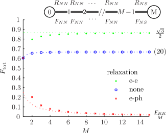
Figure 1: (Color online). Total Fano factor $F_{\text{tot}}$ for a string of $N+1$ nodes (inset), connected by $M$ connectors with the transmission eigenvalue distribution $\rho(T)=2g(\pi\sqrt{T(1-T)})^{-1}$ of chaotic cavities. Results are shown for three types of relaxation in the nodes. Inset: $M$ connectors in series.

Consider now an example setup that consists of $M-1$ nodes between two terminals “$0$” and “$M$” (see inset of Fig. 1), and attempt to calculate its differential Fano factor, $F_{\text{tot}}\equiv\frac{\partial\tilde{S}_{00}}{e\partial I}\rvert_{I=0}$ at zero temperature $T_{0}=T_{M}=0$. For simplicity of resulting expressions, we assume that all connectors are identical, sharing the same distribution $\{T_{n}^{ij}\}$ of the transmission eigenvalues.

First, if both terminals are normal, the application of Eqs. (9,10,12,14,15) is analogous to the semiclassical calculation presented in Ref. Oberholzer et al., 2002, and yields the result

$$F_{\text{tot,NN}}=\begin{cases}\frac{1}{3}+\frac{3F-1}{3M^{2}}\,,&\text{for no relaxation,}\\ \frac{F}{M}\,,&\text{for $e$-ph relaxation,}\\ \frac{\sqrt{3}}{4}\,,&\text{for $e$-$e$ relaxation, $M\rightarrow\infty$.}\end{cases}$$ (19)

This shows that the limit $M\rightarrow\infty$ corresponds to the diffusive limit, due to the isotropicity of electron momentum assumed at the nodes.

If terminal $M$ is superconducting, and relaxation is negligible, we need to apply Eqs. (9,10,12,13,14,15). In this example $b_{k}^{j}$ are then straightforward to find, $f_{L}^{j}=f_{L}^{0}$ and $f_{T}^{j}=f_{T}^{0}b_{0}^{j}+f_{T}^{M}b_{M}^{j}$ for $j=1,\ldots,M-1$. Summation in (15) then leads to a simple result

$$F_{\text{tot}}=\frac{2}{3}+\frac{(F_{NS}-\frac{2}{3})R_{NS}^{3}+\frac{M-1}{2}(F_{NN}-\frac{1}{3})R_{NN}^{3}}{[R_{NS}+(M-1)R_{NN}]^{3}}\,.$$ (20)

Here $R_{NN}$, $F_{NN}$, $R_{NS}$ and $F_{NS}$ are the resistances and differential Fano factors of the $NN$ and $NS$ connectors, as given in Eqs. (12) and (13). The result applies also for $M=1$, and in fact, for $M=2$ it is valid even if both connectors have differing $\{T_{n}^{ij}\}$. In the limit $M\rightarrow\infty$, the Fano factor again tends towards that of a diffusive contact, showing the doubling of the shot noise. de Jong and Beenakker (1994)

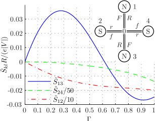
Figure 2: (Color online). Cross correlation $\tilde{S}_{13}$ between the two normal terminals changes sign as a function of contact transparency $\Gamma$, while $\tilde{S}_{24}$ and $\tilde{S}_{13}$ stay negative. Voltages are chosen $V_{1}=V_{3}=V$, $V_{2}=V_{4}=0$, and all connectors are assumed to be identical. Inset: A four-probe system. Terminals 1 and 3 are normal, 2 and 4 are superconducting. Connectors are assumed to have sub-gap resistances $R,r$ and differential Fano factors $F,f$.

Similar calculation shows that for strong inelastic e-ph scattering one has $F_{\text{tot,e-ph}}\sim F_{NN}/M$ for large $M$. For relaxation due to e-e scattering, in turn, Eq. (16b) first gives the temperature profile $T_{j}=[T_{0}^{2}+\mathcal{L}^{-1}(V_{0}^{2}-V_{j}^{2})]^{1/2}$, where $V_{j}=b_{0}^{j}V_{0}$. From Eqs. (15,12a) one then finds that $F_{\text{tot,e-e}}=\sqrt{3}/2$ for $M\rightarrow\infty$, showing again the doubling of the noise. Numerical results for the behavior at smaller $M$ are shown in Fig. 1.

It is mostly straightforward to solve the current correlations in multiterminal N-S systems, also discussed for example in Refs. Samuelsson and Büttiker, 2002b; Börlin et al., 2002; Nagaev, 2001. For the four-terminal setup shown in the inset of Fig. 2, one obtains

$$\tilde{S}_{13} =-c_{1}e(\left\lvert{V_{1}}\right\rvert+\left\lvert{V_{3}}\right\rvert+\left\lvert{V_{1}+V_{3}}\right\rvert)-c_{2}e\left\lvert{V_{1}-V_{3}}\right\rvert$$ (21)

$$c_{1} =\frac{r}{16(r+R)^{4}}[rR(1\!+\!F)+2FR^{2}+2r^{2}(1\!-\!f)]$$ (22)

$$c_{2} =\frac{r}{16(r+R)^{4}}\bigl{[}r(2r+R+2r^{2}R^{-1})+2r^{2}f$$ (23)

$$\qquad+(2+rR^{-1})(2r^{2}+4rR+R^{2})F\bigr{]}\,.$$

Here, $R=R_{NN}$, $r=R_{NS}$, $F=F_{NN}$ and $f=F_{NS}$, and the result is valid provided $\left\lvert{V_{i}}\right\rvert\ll\left\lvert{\Delta}\right\rvert$, $i=1,3$, and $T=0$. If the connectors are assumed diffusive ($F=1/3$, $f=2/3$), Eq. (21) agrees with Ref. Nagaev, 2001. One also finds that for $f>1$, the cross-correlation (21) can be positive if $R$ is small enough, Samuelsson and Büttiker (2002b) contrary to the case in normal-state circuits. For NS contacts with transparency $\Gamma$, this is satisfied for $0<\Gamma<2(\sqrt{2}-1)$, as in Refs. Torrès and Martin, 1999; Samuelsson and Büttiker, 2002b. A different example, where all four contacts are identical so that $R$ is not small, is shown in Fig. 2.

In conclusion, we discuss a simple model for the transmission of noise in multi-dot incoherent normal–superconducting structures, applying the microscopic counting field theory. The formalism produces the principle of minimal correlations, and has strong analogies with the semiclassical theory of noise in diffusive structures.

We thank W. Belzig for discussions, and P. Samuelsson and M. Büttiker for pointing out their previous work in Ref. Samuelsson and Büttiker, 2002a. TTH acknowledges the funding by the Academy of Finland.

References

• Yu. V. Nazarov and Bagrets (2002) Yu. V. Nazarov and D. A. Bagrets, Phys. Rev. Lett. 88, 196801 (2002).
• Samuelsson and Büttiker (2002a) P. Samuelsson and M. Büttiker, Phys. Rev. B 66, 201306(R) (2002a).
• Nagaev et al. (2002) K. E. Nagaev, P. Samuelsson, and S. Pilgram, Phys. Rev. B 66, 195318 (2002).
• Nagaev and Büttiker (2001) K. E. Nagaev and M. Büttiker, Phys. Rev. B 63, 081301(R) (2001).
• Belzig and Samuelsson (2003) W. Belzig and P. Samuelsson, Europhys. Lett. 64, 253 (2003).
• Blanter and Büttiker (2000) Y. A. Blanter and M. Büttiker, Phys. Rep. 336, 1 (2000).
• Belzig (2003) W. Belzig, in Quantum Noise in Mesoscopic Physics, edited by Yu. V. Nazarov (Kluwer, Dordrecht, 2003).
• Yu. V. Nazarov (1999) Yu. V. Nazarov, Superlatt. Microstruct. 25, 1221 (1999).
• Houzet and Pistolesi (2004) M. Houzet and F. Pistolesi, Phys. Rev. Lett. 92, 107004 (2004).
• de Jong and Beenakker (1994) M. J. M. de Jong and C. W. J. Beenakker, Phys. Rev. B 49, R16070 (1994).
• Büttiker (1993) M. Büttiker, J. Phys.: Condens. Matter 5, 9361 (1993).
• Beenakker (1997) C. W. J. Beenakker, Rev. Mod. Phys. 69, 731 (1997).
• Sukhorukov and Loss (1998) E. V. Sukhorukov and D. Loss, Phys. Rev. Lett. 80, 4959 (1998).
• Nagaev (1995) K. E. Nagaev, Phys. Rev. B 52, 4740 (1995).
• Oberholzer et al. (2002) S. Oberholzer, E. V. Sukhorukov, C. Strunk, and C. Schönenberger, Phys. Rev. B 66, 233304 (2002).
• Samuelsson and Büttiker (2002b) P. Samuelsson and M. Büttiker, Phys. Rev. Lett. 89, 046601 (2002b).
• Börlin et al. (2002) J. Börlin, W. Belzig, and C. Bruder, Phys. Rev. Lett. 88, 197001 (2002).
• Nagaev (2001) K. E. Nagaev, Phys. Rev. B 64, 081304(R) (2001).
• Torrès and Martin (1999) J. Torrès and T. Martin, Eur. Phys. J. B 12, 319 (1999).