On the melting of the nanocrystalline vortex matter in high-temperature superconductors

Abstract

Multilevel Monte Carlo simulations of the vortex matter in the highly-anisotropic high-temperature superconductor Bi₂Sr₂CaCu₂O₈ were performed. We introduced low concentration of columnar defects satisfying $B_{\phi}\leq B$. Both the electromagnetic and Josephson interactions among pancake vortices were included. The nanocrystalline, nanoliquid and homogeneous liquid phases were identified in agreement with experiments. We observed the two-step melting process and also noted an enhancement of the structure factor just prior to the melting transition. A proposed theoretical model is in agreement with our findings.

Recently there were several experiments reporting on some interesting features of the vortex matter melting transition in Bi₂Sr₂CaCu₂O₈ (BSCCO) in the present of columnar defects (CDs) Banerjee ; Menghini ; Banerjee2 . In particular, these experiments consider the case that the density of the CDs does not exceed the density of flux-lines (FLs). Denoting the “matching field” by $B_{\phi}=n_{cd}\phi_{0}$, where $n_{cd}$ is the number of CDs per unit area and $\phi_{0}=hc/2e$ is the flux quantum, we are particularly interested in $B_{\phi}\leq B$. The CDs are created artificially by irradiating the sample by highly energetic heavy ions, like 1 GeV Pb ions, which produce tubes of non-conducting damaged material. The number of CDs can be controlled by the amount of irradiation. We assume that CDs and the applied magnetic field are aligned with the c-axis of the single crystal sample. The limit $B\gg B_{\phi}$ corresponds to the formation of the Bose glass phase at low temperature where vortices are situated on the randomly placed CDs Blatter ; Nelson ; Radzihovsky ; Kees . On the other hand, for $B<B_{\phi}$ the picture that emerged from experiments Banerjee ; Menghini ; Banerjee2 and from simulations Tyagi ; Dasgupta is that of the “crystallites in the pores”, also referred to as the “porous” vortex solid. At low temperatures a skeleton (or matrix) of vortices localized on CDs is formed, while the excess (interstitial) FLs form hexagonal crystallites in the lacuna between CDs. Thus this phase has a short ranged translational order, which extends to a distance of the order of a typical pore size.

As the temperature is increased, and if the magnetic field is large enough, this heterogeneous structure melts in two stages: first the crystallites in the pores melt into a nanoliquid while the skeleton remain intact, and subsequently the skeleton melts and the liquid becomes homogeneous. When the magnetic field is lowered (but still greater than $B_{\phi}$) these two transitions coincide into one. This is usually associated with a kink in the first order melting line. The first stage melting of the crystallites is observed in the experiments as a step in the equilibrium local magnetization Pastoriza ; Zeldov ; Schilling and in the simulations as a sharp increase in the transverse fluctuations of the FLs, among other signatures. The second transition was not observed in the experiments as a similar jump in the magnetization or another equilibrium property. It was observed in transport measurement Banerjee2 involving transport currents with alternating polarity. This establishes the transition as dynamical in nature. It remains to be established that this is also an equilibrium thermodynamic transition. In order to support this assertion it was argued Banerjee2 that the second “delocalization” transition is associated with the restoration of a broken longitudinal gauge symmetry. However, at this time it cannot be ruled out that the second transition is only a crossover associated with a gradual equilibrium change over a finite range of temperatures.

The aim of this work was to try to observe the sequence of the two transitions and in particular the two different kinds of liquid phases in numerical simulations. Some of the advantages of using Monte Carlo simulations are that one can control all the interactions precisely, and one can take microscopic pictures and measure physical quantities that are difficult to measure in experiments, like the magnitude of the transverse fluctuations of FLs or the amount of their entanglement. A main disadvantage is that the system simulated is small and hence phase transitions are always broadened and are not as sharp as those observed in real experiments.

The method we are using is a multilevel Monte Carlo simulation as reported in earlier publications Tyagi . In a highly anisotropic material like BSSCO the basic degrees of freedom are pancake vortices rather than string-like FLs. A stack of pancakes make a FL and nearest neighbor pancakes along the z-direction interact via the Josephson interaction (here we used the approximation recently derived in Ref. Goldschmidt, ). In addition there is a long range electromagnetic interaction among all pairs of pancakes Clem , that is repulsive when the two pancakes reside in the same plane and attractive otherwise. Periodic boundary conditions are implemented in all directions. Similar to simulations of systems of bosons Ceperley , we implement permutations when connecting FLs between the top and bottom planes of the simulation slab. Most simulations involved $6\times 6\times 36$ pancakes making up 36 FLs in 36 planes (some simulations involved 64 FLs). Extensive simulations were carried out for the case of $B_{\phi}=50$ G. Since we keep the number of FLs fixed at $36$ this means that the number of CDs vary as a function of the magnetic field such that $N_{cd}=36~{}B_{\phi}/B$. The simulations were carried out for fields $B=50$ G to $200$ G and thus $N_{cd}/N_{FL}$ vary between $100\%$ to $25\%$. We simulated between $T=60$ K to $79$ K with one degree increments. The critical temperature for BSCCO was assumed to be $T_{c}=90$ K. Other parameters used were $\lambda(0)=1700$ Å (penetration depth), $\xi(0)=30$ Å (correlation length), $d=15$ Å (CuO₂ plane separation), $\gamma=375$ (anisotropy). We assumed that $\lambda$ and $\xi$ have temperature dependence that is proportional to $(1-T/T_{c})^{-1/2}$.

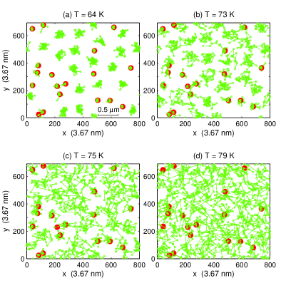
Figure 1: (color online) Snapshots of the FLs and CDs (green open circles) configurations for $B=100$ G. The pancakes in 36 planes are projected onto a single plane. Pancakes belonging to the same FL are shown to be connected. (a) The nanocrystal phase characterized by hexagonal order in the pores. (b) Just before the melting. A slight enhancement of the structure factor (see text). (c) Nanoliquid phase. The pores have melted but not the skeleton. (d) Homogeneous liquid, full entanglement.

An important ingredient of the simulation is determining how to model the interaction between pancakes and CDs in a realistic way. There are two major sources of pinning: core and electromagnetic pinning. Core pinning Blatter arises when the vortex core overlaps with a normal state inclusion similar to the one inside a CD. Since condensation energy is lost in the vortex core, part or all of this energy is restored when a vortex resides inside a CD. Electromagnetic pinning arises Buzdin ; Mkrtchyan when the supercurrent pattern around the vortex is disturbed by the non-conducting defect. These two mechanisms combine together to yield the expression for the potential energy at a distance $R$ away from the CD as felt by an individual pancake Blatter ; Mkrtchyan :

$$V(R)\approx\left\{\begin{array}[]{c}\epsilon_{0}d\ \ln\left[1-\left(\frac{r_{r}}{R+\xi/\sqrt{2}}\right)^{2}\right],\ \ R>r_{r},\\ \epsilon_{0}d\ \ln\left[1-\left(\frac{r_{r}}{r_{r}+\xi/\sqrt{2}}\right)^{2}\right],\ \ R<r_{r},\end{array}\right.$$ (3)

where $\epsilon_{0}=\phi_{0}/(4\pi\lambda)^{2}$ is the energy scale, and $r_{r}$ is the radius of the CD. The long range tail contributing $\approx-\epsilon_{0}dr_{r}^{2}/R^{2}$ is due mainly to the electromagnetic pinning and the short range flat region of depth $\approx\epsilon_{0}d$ is due to the combined effects of electromagnetic and core pinning. If $r_{r}<\sqrt{2}\xi$ a slightly different expression, $V(R)\approx-0.5\epsilon_{0}dr_{r}^{2}/(R^{2}+2\xi^{2})$, with a similar long tail should be used instead Blatter . The importance of the long tail was realized recently Lopatin as leading to a dependence $B_{dl}\sim\exp(-T/T_{0})$ instead of $B_{dl}\sim\exp(-T^{2}/T_{0}^{2})$, leading to the decoupling of FLs from CDs at a higher temperature than previously thought Lopatin .

After experimenting with CDs of different radii $10$ nm $\leq r_{r}\leq 30$ nm we concluded that in order to obtain a good agreement with experimental results we needed to choose $r_{r}\approx 30$ nm in which case the formula given by Eq. (3) is the correct one. Different heavy ions with different energies give rise to tracks of various sizes, normally reported to be in the range of $4-20$ nm in diameter. It may be that the actual damage caused by a track exceed its apparent size, thus leading to a higher effective radius.

We now turn to the results of the actual simulations. Most simulations were done on the Pittsburgh supercomputing cluster and involved averaging over 10 realizations of the disorder at each temperature. Typically we ran 4,000,000 Monte Carlo steps for equilibration and 2,000,000 for measurements. Snapshots are depicted in Fig. 1 at four representative temperatures. The nanocrystal, (a), nanoliquid (c) and homogeneous liquid (d) phases are clearly distinguishable. In addition we display an intermediate picture (b) taken during the broadened melting transition where the structure factor slightly increases (see later discussion of Fig. 4) due to a better rearrangement of the FLs than just before the conclusion of the melting. In the simulations, when CDs are present, the transition is broadened probably by the fact that pores of different sizes don’t melt simultaneously especially in a finite size system.

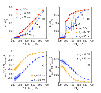
Figure 2: (color online) Measured quantities for $B=100$ G. The pristine case and the case of CDs with radii of 20 and 30 nm are shown. (a) Mean square transverse fluctuations of the FLs. For CDs of radius 30 nm the melting and delocalization transitions are indicated with arrows. The first stage melting occurs for $C_{L}^{2}\approx 0.1$ where $C_{L}$ is the Lindemann parameter. (b) Number of loops of size greater than unity. A measure of FL entanglement. (c) Binding energy per pancake between FLs and CDs. (d) Number of capture pancakes per CD per plane.

In Fig. 2 we display different measurable quantities that are indicators of the melting transitions. The red solid circles represent the pristine system with no CDs and the melting appears sharp both for the magnitude of the transverse fluctuations (a) and for the measure of entanglement (b), given as the fraction of FLs not ending on themselves by the periodic boundary conditions in the z-direction but rather, due to the proliferation of permutations resulting in composite loops made up of several individual segments. For the 30 nm CDs the two stage melting is quite evident. For the transverse fluctuations we first see a broad flat part ending in the first melting and then a second kink signaling the approach of the fluctuations toward the pristine value that indicates the melting of the skeleton. These transitions are marked by the arrows. The flat part and the final kink are also evident in Fig. 2 (b). For 20 nm the flat part is shorter and both transitions occur closer to the pristine melting. In subplots (c) and (d) we display the binding energy per pancake and the fraction of trapped pancakes per CD per plane. Both these quantities become very small at the delocalization transition. From here onward we limit the discussions to CDs of radius of 30 nm.

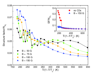
Figure 3: (color online) Normalized structure factor at the first Bragg peak for different values of the magnetic field. The enhancement of the structure factor just below the field-dependent melting transition is apparent. The inset shows the pristine vs. irradiated sample for $B=150$ G.

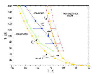
Figure 4: (color online) Phase diagram in the $T-B$ plane as suggested from the results of the simulations.

In Fig. 3 we display the structure factor as a function of the reduced temperature for different fields. The structure factors is not a good indicator of the melting transition when CDs are present since the random skeleton make it very low to begin with and the transition is broadened and becomes second order or weakly first order. We can see clearly the rise of the structure factor during the onset of the melting of the nanocrystalline solid since it becomes easier for the interstitial vortices to find better positions that are closer to hexagonal order before the full melting occurs. We found evidence for this by looking at snapshots at this temperature range. See e.g. Fig. 1 (b), although there are more striking examples. A similar effect was discussed in Ref. Tyagi, for weaker columnar pins of smaller radius. The inset shows the sharp pristine melting transition for $B=150$ G as indicated by the step in the structure factor in contrast to the much weaker decline in the case of columnar pins.

In Fig. 4 we display the phase diagram as it emerges from the results of the simulations. The green line connecting the empty circles is the location of the melting transition for the pristine system. The blue line connecting the filled squares denote the melting of the “irradiated” systems when CDs of radius 30 nm are present. This line denotes the conclusion of the melting of the nanocrystalline solid which now becomes a nanoliquid. The horizontal blue bars denote the broadening of the first stage melting characterized by the flat sections in Fig. 2 (a) and (b). The two red lines (solid and dashed) connected by horizontal error bars denote the second stage melting of the skeleton which can be determined to a precision of about 2 K. Note that for $B_{\phi}=50$ G the two transitions merge together. The kink in the first-stage melting is defined by the point of largest shift of the melting temperature from its pristine value and this occurs at $B\approx 100$ G. A change in slope of the melting line is observed there. In our simulation at this point the two melting transitions do not yet coincide. This is similar to the experimental results reported in Ref. Banerjee2, for $B_{\phi}=60$ G. We also show in Fig. 4 the prediction of a simple theoretical model described as follows:

The cage model is often used to get a rough estimate of the melting transitionCrabtree . For a FL trapped by a CD we add the binding energy between the FL and the CD to the harmonic cage potential. Thus the free-energy functional for a single FL is given by:

$$F=\int_{0}^{L}dz\left[\frac{\epsilon_{1}}{2}\left(\frac{d\bm{r}(z)}{dz}\right)^{2}+U(\bm{r})+\frac{1}{2}k\bm{r}^{2}\right],$$ (4)

where $U(\bm{r})$ is the binding energy to the CD ($U(r)=V(r)/d$ as given in Eq.(1) above), $\epsilon_{1}$ is the tilt modulus and $k\approx\epsilon_{0}/a_{0}^{2}$ where $a_{0}=\sqrt{\phi_{0}/B}$ is the mean separation between FLs. We now utilize the mapping of this model to a quantum particle in a potential where the correspondence is $\hbar\rightarrow T$, $m\rightarrow\epsilon_{1}$ and $z$ becomes the imaginary time. In the limit $L\rightarrow\infty$ the particle is at zero temperature and its energy is given by the ground state of the corresponding Schrodinger equation

$$\left[-\frac{T^{2}}{2\epsilon_{1}}\bm{\nabla}^{2}+U(\bm{r})+\frac{1}{2}k\bm{r}^{2}\right]\psi(\bm{r})=E\psi(\bm{r}),$$ (5)

in two spatial dimensions. We have chosen the following value for $\epsilon_{1}$

$$\epsilon_{1}\approx\epsilon_{0}\left(\frac{1.55+\ln(\lambda/d)}{\gamma^{2}}+\frac{d^{2}}{\lambda^{2}}\right).$$ (6)

The first term approximately represents the contribution of the Josephson interaction Koshelev ; Goldschmidt and the second term results from the electromagnetic interaction Clem . We solved the Schrodinger equation numerically using either the shooting method or alternatively the matrix method. The equation reduces to a one-dimensional radial equation. The melting transition is obtained by calculating the expectation value of $r^{2}$ and using the Lindemann criterion with $C_{L}^{2}\approx 0.1$ to identify the melting temperature. For $U=0$ we obtained the approximation to the pristine melting curve displayed in Fig. 4. Including $U(r)$ we obtain the result for $B_{dl}$, the field corresponding to the skeleton melting. We have also solved numerically the Schrodinger equation without the cage and used the resulting energy and localization length to reconstruct $B_{dl}$ following Lopatin and Vinokur Lopatin . The result is reasonable but the agreement is not as good than the method described above. The delocalization field obtained from the simulation and from the solution of the Schrodinger equation satisfies approximately $B_{dl}\sim\exp(-T/T_{0})$ with $T_{0}\approx 3$ K. This line is somewhat steeper than the experimental result Banerjee2 , but this is also true for the melting line that is flatter in the experiment. This is most likely due to the fact that experimentally pristine samples contain a certain amount of point defects that lower the melting temperature and which are even more effective in lower temperatures and higher fields.

Conclusions - In this paper we used the multilevel Monte Carlo method to simulate the pancake vortices in the highly anisotropic superconductor BSCCO in the presence of columnar defects of low concentration. When the applied field is larger than the matching field we have found evidence for a sequence of two melting transitions, one associated with the melting of crystallites and the second with the demise of the skeleton - the FLs attached to the CDs. Of course this is not a conclusive evidence that the latter transition is a true thermodynamic transition. The agreement with experiment is amazingly good for a system of 1296 pancakes when averaging over 10 realizations of the disorder and display most of the salient features found in the experiments. In addition we found a new feature - a slight but noticeable enhancement of the structure factor just prior to the melting transition when CDs are present. This enhancement might be observed in experiments using small-angle neutron scattering technique (SANS) which can effectively be used to measure the structure factor.

Acknowledgments - This work is supported by the US Department of Energy (DOE), Grant No. DE-FG02-98ER45686. Some of the simulations were done at the Pittsburgh Supercomputing center under Grant No. DMR950009P. YYG would like to thank Eli Zeldov for useful discussions and for his hospitality at his lab at the Weizmann institute.

References

- (1) S. S. Banerjee et al., Phys. Rev. Lett. 90, 087004 (2003).
- (2) M. Menghini et al., Phys. Rev. Lett. 90, 147001 (2003).
- (3) S. S. Banerjee et al., Phys. Rev. Lett. 93, 097002 (2004).
- (4) G. Blatter et al., Rev. Mod. Phys. 66, 1125 (1994).
- (5) D.R. Nelson and V.M. Vinokur, Phys Rev. Lett. 68, 2398 (1992).
- (6) L. Radzihovsky, Phys. Rev. Lett. 74, 4923 (1995).
- (7) C. J. Van der Beek et al., Phys. Rev. Lett. 86, 5136 (2001).
- (8) S. Tyagi and Y. Y. Goldschmidt, Phys. Rev. B 67, 214501 (2003); ibid B70, 024501 (2004).
- (9) C. Dasgupta and O.T. Valls, Phys. Rev. Lett. 91,127002 (2003).
- (10) H. Pastoriza et al., Phys. Rev. Lett. 72, 2951 (1994).
- (11) E. Zeldov et al., Nature 375, 373 (1995).
- (12) A. Schilling et al., Nature 382, 791 (1996).
- (13) A.V. Lopatin and V.M. Vinokur, Phys. Rev. Lett. 92, 067008 (2004).
- (14) Y. Y. Goldschmidt and S. Tyagi, Phys. Rev. B 71, 014503 (2005)
- (15) J. R. Clem, Phys. Rev. B 43, 7837 (1991).
- (16) D. M. Ceperley, Rev. Mod. Phys. 67, 279 (1995).
- (17) G. S. Mkrtchyan and V. V. Schmidt, Sov. Phys. JETP 34, 195 (1972).
- (18) A. Buzdin and D. Feinberg, Physica C 235-240, 2755 (1994).
- (19) G. W. Crabtree and D. R. Nelson, Physics Today 50, 38 (1997).
- (20) A. E. Koshelev, Phys. Rev. B 48, 1180 (1993).