On the Mott formula for thermopower of non-interactions electrons in quantum point contacts

Abstract

We calculate the linear response thermopower $S$ of a quantum point contact using the Landauer formula and therefore assume non-interacting electrons. The purpose of the paper, is to compare analytically and numerically the linear thermopower $S$ of non-interacting electrons to the low temperature approximation, $S^{(1)}=(\pi^{2}/3e)k_{\rm B}^{2}T\partial_{\mu}[\ln G(\mu,T=0)]$, and the so-called Mott expression, $S^{\rm M}=(\pi^{2}/3e)k_{\rm B}^{2}T\partial_{\mu}[\ln G(\mu,T)]$, where $G(\mu,T)$ is the (temperature dependent) conductance. This comparison is important, since the Mott formula is often used to detect deviations from single-particle behavior in the thermopower of a point contact.

1 Introduction

A narrow constriction in for example a two dimensional electron gas makes a small cannel between two electron reservoirs. This constriction is called a quantum point contact[1]. The width of the cannel can be controlled by a gate voltage and by applying a small bias the phenomenon of quantized conductance as a function of the width(i.e. gate voltage) is observed at low temperatures[2]. This quantization is due to the wave nature of the electronic transport through the short ballistic point contact. Experimentally[3, 4, 5, 6, 7], it is also possible to heat up one of the sides of the point contact and thereby producing a temperature difference $\Delta T$ across the contact, which in turn gives an electric current (and a heat current) though the point contact. By applying a bias $V$ in the opposite direction of the temperature difference $\Delta T$ the two contributions to the electric current $I$ can be make to cancel, which defines the thermopower $S$ as

$$S=\left.-\lim_{\Delta T\rightarrow 0}\frac{V}{\Delta T}\right|_{I=0}.$$ (1)

For a quantum point contact, the thermopower as a function of gate voltage has a peak every time the conductance plateau changes from one subband of the transverse quantization to the next[5, 8].

In order to compare experiment and theory for the thermopower of a point contact the so-called Mott formula,

$$S^{\rm M}\propto\partial_{V_{g}}\left[\ln G(V_{g},T)\right],$$ (2)

is often a valuable toll, because by differentiating the experimentally found conductance $G(V_{g},T)$ with respect to the gate voltage $V_{g}$ one can see, if there is more information in the thermopower that in the conductance. This additional information could for example be many body effects[7], since $S^{\rm M}$ is an approximation to the single-particle thermopower. Note that this approximation is independent of the specific form of the transmission $\mathcal{T}(\varepsilon)$ though the point contact. It is the purpose of this paper, to determine the validity of the Mott approximation $S^{\rm M}$ and thereby decide if it is really deviations from single-particle behavior the experiments[6, 7, 9] observe or rather an artefact of this approximation.

2 Thermopower from the Landauer formula

For the sake of completeness, we begin by deriving the single-particle thermopower formula in linear response to the applied bias $V$ and temperature difference $\Delta T$. The current though a ballistic point contact is found from the Landauer formula[10][p.111, Eq.(7.30)]:

$$I=\frac{2e}{h}\int_{0}^{\infty}\!\!\!\!\textrm{d}\varepsilon\mathcal{T}(\varepsilon)[f^{0}_{L}(\varepsilon)-f^{0}_{R}(\varepsilon)],$$ (3)

where $\mathcal{T}(\varepsilon)$ is the transmission and $f^{0}_{i}(\varepsilon)$ is the Fermi function for the right/left ($i=R,L$) lead. The Landauer formula assumes non-interacting electrons and therefore so will the derived thermopower formula. When a small bias $V=(\mu_{L}-\mu_{R})/(-e)$ and temperature difference $\Delta T=T_{L}-T_{R}$ is applied, we can expand the distribution functions around $\mu$, $T$ as ($|\Delta T|/T\ll 1$ and $|eV|\ll\mu$):

$$f^{0}_{i}(\varepsilon)\simeq f^{0}(\varepsilon)-\partial_{\varepsilon}f^{0}(\varepsilon)(\mu-\mu_{i})-(\varepsilon-\mu)\partial_{\varepsilon}f^{0}(\varepsilon)\frac{T-T_{i}}{T},$$ (4)

where $f^{0}(\varepsilon)$ is the Fermi function with the equilibrium chemical potential $\mu$ and temperature $T$ and $i=L,R$. To obtain the thermopower eq.(1) we insert the distribution functions in eq.(3) and set it equal to zero and obtain:

$$S(\mu,T)=\frac{1}{eT}\frac{\int_{0}^{\infty}\!\textrm{d}\varepsilon\mathcal{T}(\varepsilon)(\varepsilon-\mu)[-\partial_{\varepsilon}f^{0}(\varepsilon)]}{\int_{0}^{\infty}\!\textrm{d}\varepsilon\mathcal{T}(\varepsilon)[-\partial_{\varepsilon}f^{0}(\varepsilon)]},$$ (5)

which is our exact single-particle formula.

3 Approximations to the thermopower and there validity

3.1 The low temperature (first order) approximation

For $T=0$ we have $-\partial_{\varepsilon}f^{0}(\varepsilon)=\delta(\varepsilon-\mu)$, so the numerator in eq.(5) is zero, i.e. $S(\mu,T=0)=0$. For temperatures $k_{\rm B}T$ much lower than the scale of variation of $\mathcal{T}(\varepsilon)$ and $k_{\rm B}T\ll\mu$, we can expand $\mathcal{T}(\varepsilon)$ around $\mu$ to first order (i.e. a Sommerfeld expansion) to obtain:

$$S^{(1)}(\mu,T)=\frac{\pi^{2}}{3}\frac{k_{\rm B}}{e}k_{\rm B}T\frac{1}{\mathcal{T}(\mu)}\frac{\partial\mathcal{T}(\mu)}{\partial\varepsilon}=\frac{\pi^{2}}{3}\frac{k_{\rm B}}{e}k_{\rm B}T\frac{1}{G(\mu,T=0)}\frac{\partial G(\mu,T=0)}{\partial\mu},$$ (6)

where $G(\mu,T=0)$ is the conductance for zero temperature, i.e. $G(\mu,T=0)=\frac{2e^{2}}{h}\mathcal{T}(\mu)$.

3.2 The Mott approximation and analytical considerations of its validity

The Mott approximation [6, 7] is

$$S^{\rm M}(\mu,T)=\frac{\pi^{2}}{3}\frac{k_{\rm B}}{e}k_{\rm B}T\frac{1}{G(\mu,T)}\frac{\partial G(\mu,T)}{\partial\mu},$$ (7)

where $G(\mu,T)$ is the temperature dependent conductance

$$G(\mu,T)=\frac{2e^{2}}{h}\int_{0}^{\infty}\!\textrm{d}\varepsilon\mathcal{T}(\varepsilon)[-\partial_{\varepsilon}f^{0}(\varepsilon)].$$ (8)

The form of $S^{\rm M}$ stated in eq.(2) assumes that the chemical potential and gate voltage are linear dependent. The Mott approximation to the single-particle thermopower eq.(5) and its range of validity is not so obvious compared to the approximation of the first order Sommerfeld expansion eq.(6).

One way of comparing $S$ from eq.(5) and $S^{\rm M}$ is to differentiate eq.(8) to obtain (assuming that $\mathcal{T}(\varepsilon)$ is independent of $\mu$):

$$S^{\rm M}(\mu,T)=\frac{\pi^{2}}{3}\frac{k_{\rm B}}{e}\frac{1}{G(\mu,T)}\int_{0}^{\infty}\!\textrm{d}\varepsilon\mathcal{T}(\varepsilon)\tanh\left(\frac{\varepsilon-\mu}{2k_{\rm B}T}\right)[-\partial_{\varepsilon}f^{0}(\varepsilon)],$$ (9)

i.e. by using the Mott formula we approximate $(\varepsilon-\mu)/k_{\rm B}T$ in the integral by $(\pi^{2}/3)\tanh[(\varepsilon-\mu)/(2k_{\rm B}T)]$.

To compare $S$ and $S^{\rm M}$ in another way, we observe that for low temperatures $k_{\rm B}T\ll\mu$ the Mott approximation $S^{\rm M}$ simplifies to $S^{(1)}$ eq.(6), because $G(\mu,T)\rightarrow\frac{2e^{2}}{h}\mathcal{T}(\mu)$ for $T\rightarrow 0$, i.e. $S(\mu,T)=S^{(1)}(\mu,T)=S^{\rm M}(\mu,T)$ for $k_{\rm B}T/\mu\rightarrow 0$. Therefore, we compare $S$ and $S^{\rm M}$ by expanding both quantities in orders of $k_{\rm B}T$ and comparing order by order. Using

$$\mathcal{T}(\varepsilon)=\sum_{n=0}^{\infty}\frac{1}{n!}\frac{\partial^{n}\mathcal{T}(\mu)}{\partial\varepsilon^{n}}(\varepsilon-\mu)^{n},$$ (10)

we can exactly rewrite eq.(8)

$$G = \frac{2e^{2}}{h}\sum_{n=0}^{\infty}\frac{1}{n!}\frac{\partial^{n}\mathcal{T}(\mu)}{\partial\varepsilon^{n}}\int_{0}^{\infty}\!\textrm{d}\varepsilon(\varepsilon-\mu)^{n}[-\partial_{\varepsilon}f^{0}(\varepsilon)]$$ (11)

$$= \frac{2e^{2}}{h}\sum_{n=0}^{\infty}\frac{1}{n!}\frac{\partial^{n}\mathcal{T}(\mu)}{\partial\varepsilon^{n}}(k_{\rm B}T)^{n}\mathfrak{B}_{n}\Big{(}\frac{\mu}{k_{\rm B}T}\Big{)},$$

where ($y=(\varepsilon-\mu)/k_{\rm B}T$)

$$\mathfrak{B}_{n}\Big{(}\frac{\mu}{k_{\rm B}T}\Big{)}\equiv\int_{-\frac{\mu}{k_{\rm B}T}}^{\infty}\!\!\!\!\textrm{d}y\frac{y^{n}}{4\cosh^{2}(y/2)}\quad\rightarrow\quad I_{n}\equiv\int_{-\infty}^{\infty}\!\!\!\!\textrm{d}y\frac{y^{n}}{4\cosh^{2}(y/2)}\quad\textrm{for}\ k_{\rm B}T\ll\mu,$$ (12)

where we note that $I_{2n+1}=0$ for all integer $n$. Numerically it turns out, that $\mathfrak{B}_{n}(\mu/k_{\rm B}T)/\mathfrak{B}_{n}(0)\simeq 0$ for $\mu\gtrsim(10+n)k_{\rm B}T$ as seen in figure 1. The integral $I_{n}$ can be calculated and the first values are:

$$I_{0}=1,\ I_{2}=\frac{\pi^{2}}{3},\ I_{4}=\frac{7\pi^{4}}{15},\ I_{6}=\frac{31\pi^{6}}{21},\ I_{8}=\frac{127\pi^{8}}{15},\ \ldots$$ (13)

Figure 1: (Left): The approximation in eq.(12) is pictured for odd integer values of $n$ from 1(left) to 19(right) in $\mathfrak{B}_{n}(\mu/k_{\rm B}T)$. We note that $\mathfrak{B}_{n}(\mu/k_{\rm B}T)/\mathfrak{B}_{n}(0)\simeq 0$ for $\mu\gtrsim(10+n)k_{\rm B}T$. (Right): The numerical values of the factors in the series expansions of the Mott approximation eq.(15) (lower) and the exact linear single-particle series expansion eq.(16 ) (upper).

Using the approximation eq.(12) we get

$$G(\mu,T)\simeq\frac{2e^{2}}{h}\sum_{n=0}^{\infty}\frac{1}{(2n)!}\frac{\partial^{2n}\mathcal{T}(\mu)}{\partial\varepsilon^{2n}}I_{2n}(k_{\rm B}T)^{2n}.$$ (14)

This leads to a Mott approximation to the thermopower for low temperatures as

$$S^{\rm M}(\mu,T)\simeq\frac{k_{\rm B}}{e}\frac{1}{G(\mu,T)}\frac{2e^{2}}{h}\left[\sum_{n=0}^{\infty}\frac{I_{2}I_{2n}}{(2n)!}\frac{\partial^{2n+1}\mathcal{T}(\mu)}{\partial\varepsilon^{2n+1}}(k_{\rm B}T)^{2n+1}\right].$$ (15)

Writing the exact single-particle thermopower $S$ eq.(5) by using eq.(10) and the approximation of low temperatures eq.(12), we get

$$S(\mu,T)\simeq\frac{k_{\rm B}}{e}\frac{1}{G(\mu,T)}\frac{2e^{2}}{h}\left[\sum_{n=0}^{\infty}\frac{I_{2n+2}}{(2n+1)!}\frac{\partial^{2n+1}\mathcal{T}(\mu)}{\partial\varepsilon^{2n+1}}(k_{\rm B}T)^{2n+1}\right].$$ (16)

We see that both formulas only have odd term in $k_{\rm B}T$ and the first order term is the same (which is $S^{(1)}$). However, none of the higher order terms are the same and on figure 1(right) the different numerical factors of the two series expansions are seen to behave very differently as the power of $k_{\rm B}T$ grows:

$$\frac{I_{2n+2}}{(2n+1)!}\sim 4.00\times n+\frac{\pi^{2}}{3}\quad\textrm{and}\quad\frac{I_{2}I_{2n}}{(2n)!}\rightarrow 6.58\ \ \textrm{for}\ n\gtrsim 10.$$ (17)

So the Mott approximation is better the smaller the temperature compared to $\mu$, but not a bad approximation for moderate temperatures (i.e. $k_{\rm B}T$ comparable to other energy scales) as we shall see numerically. Note that if the approximation eq.(12) is not valid, then we have all powers of $k_{\rm B}T$.

4 Comparison of the approximations to the exact single-particle thermopower from numerical integration

We need a specific model for the transmission to do a numerical comparison of $S$ from eq.(5) to $S^{\rm M}$ and $S^{(1)}$. Using a harmonic potential in the point contact, i.e. a saddle point potential, a transmission in the form of a Fermi function can be derived[13]:

$$\mathcal{T}(\varepsilon)=\sum_{n=1}^{n_{\rm max}}\frac{1}{\exp(\frac{n\varepsilon_{0}-\varepsilon}{\varepsilon_{s}})+1},$$ (18)

where $\varepsilon_{s}$ is the smearing of the transmission between the steps and $\varepsilon_{0}$ is the length of the steps (often called subband spacing). In terms of the harmonic potential $V(x,y)=\textrm{const}-m\omega_{x}^{2}x^{2}/2+m\omega_{y}^{2}y^{2}/2$, where $x$ is along the cannel, we have $\varepsilon_{0}=\hslash\omega_{y}$ and $\varepsilon_{s}=\hslash\omega_{x}/(2\pi)$. Other functional forms of $\mathcal{T}$ have also been tested, but as along as they have the same graphical structure (such as for example a $\tanh$ dependence) the same conclusions are obtained.

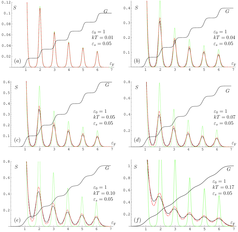
Figure 2: Thermopower $S$ from numerical integration of eq.(5) (black solid line), the Mott formula $S^{\rm M}$ eq.(7) (red dashed line) and the first order approximation $S^{(1)}$ eq.(6) (green dotted line). From figure (a) to (f) the temperature is turned from the low temperature regime $k_{\rm B}T<\varepsilon_{s}$ to $k_{\rm B}T>\varepsilon_{s}$ in small steps. The smearing of the transmission $\varepsilon_{s}$ is keep constant and note that $\varepsilon_{s},k_{\rm B}T\ll\varepsilon_{0}$ and $\varepsilon_{s},k_{\rm B}T\ll\varepsilon_{\rm F}$ in all the graphs. The thermopowers are all in units of $k_{\rm B}/e$, but note the different magnitudes of the thermopower from (a) to (f). The conductance $G$ is shown (in arbitrary units) for comparison.

Three regimes of temperatures relevant to experiments are investigated numerically:

$$k_{\rm B}T<\varepsilon_{s}\ (\textrm{fig.\ref{fig:Thermopower} (a)}),\quad k_{\rm B}T\sim\varepsilon_{s}\ (\textrm{fig.\ref{fig:Thermopower} (b-d)})\quad\textrm{and}\quad k_{\rm B}T>\varepsilon_{s}\ (\textrm{fig.\ref{fig:Thermopower} (e-f)}).$$ (19)

The thermopower $S$ for the transmission model eq.(18) is found from numerical integration of eq.(5) and compared to the Mott approximation $S^{\rm M}$ eq.(7) and the first order approximation $S^{(1)}$ eq.(6). In all three regimes, we have a staircase conductance, so $k_{\rm B}T\ll\varepsilon_{0}$, and $G(\mu,T)$ is also shown in the figures (in arbitrary units) for comparison. Furthermore, $\mu=\varepsilon_{\rm F}$ is of order $\varepsilon_{0}$, so the approximation $k_{\rm B}T\ll\varepsilon_{\rm F}$ used for example in eq.(12) is indeed very good. Note that all energies in the figures are given in units of the step length $\varepsilon_{0}$.

The information obtained from the numerical calculations is the following. Figure 2(a-b) shows that for $k_{\rm B}T$ being the lowest energy scale both approximations work very well as expected from the analytical considerations. When the temperature becomes comparable to the smearing of the steps, $k_{\rm B}T\sim\varepsilon_{s}$, the Culter-Mott formula works well and better than the first order approximation as seen in fig. 2(b-d). For $k_{\rm B}T$ bigger than $\varepsilon_{s}$ the Mott approximation still works quit well whereas $S^{(1)}$ is not a good approximation anymore. The reason for the Mott approximation to work well is found in the similar terms in the analytic temperature expansions eq.(15) and (16). Note that as $k_{\rm B}T$ increases both $S^{(1)}$ and $S^{\rm M}$ show a tendency to overestimate $S$ at the peaks and underestimate it at the valleys.

In summary, we have found that the Mott approximation to the single-particle thermopower is a fairly good approximation as along as the temperature is smaller than the Fermi level, but $k_{\rm B}T$ can be both compatible and larger than the smearing of the transmission $\varepsilon_{s}$. However, to rule out any doubt one could use an experimental determination of $\mathcal{T}(\varepsilon)$ from the (very low temperature) conductance to find the single-particle thermopower from eq.(5), which could perhaps give an interesting comparison to the experimental result. Thereby one would obtain an even more convincing statement of deviations from single-particle behavior in the thermopower.

5 Acknowledgements

We will like to thank James T. Nicholls for sharing his experimental results with us and for discussions of the thermopower in point contacts in general.

References

References

• [1] H.Β V. Houten and C. Beenakker, Phys. Today july, 22 (1996), for an minor review.
• [2] B.Β J. van Wees etΒ al., Phys. Rev. Lett. 60, 848 (1988).
• [3] L.Β W. Molenkamp etΒ al., Phys. Rev. Lett. 65, 1052 (1990).
• [4] L.Β W. Molenkamp etΒ al., Phys. Rev. Lett. 68, 3765 (1992).
• [5] H. van Houten, L.Β W. Molenkamp, C.Β W.Β J. Beenakker, and C.Β T. Foxon, Semicond. Sci. Technol. 7, B215 (1992).
• [6] N.Β J. Appleyard etΒ al., Phys. Rev. Lett. 81, 3491 (1998).
• [7] N.Β J. Appleyard etΒ al., Phys. Rev. B 62, 16275(R) (2000).
• [8] P. Streda, J. Phys.: Condens. Matter 1, 1025 (1989).
• [9] Y.Β Y. Proskuryakov etΒ al., (unpublish) (2004).
• [10] H. Bruus and K. Flensberg, Many-Body Quantum Theory in Condensed Matter Physics, Oxford Graduate Texts, 1st ed. (Oxford University press, New York, 2004).
• [11] N.Β F. Mott and H. Jones, The Theory of the Properties of Metals and Alloys, 1st ed. (Clarendon, Oxford, 1936).
• [12] M. Cutler and N.Β F. Mott, Phys. Rev. 181, 1336 (1969).
• [13] M. B$\ddot{\textrm{u}}$ttiker, Phys. Rev. B 41, 7906(R) (1990).