$\bm{N}$-leg integer-spin ladders and tubes in commensurate external fields:
Nonlinear sigma model approach

Abstract

We investigate the low-energy properties, especially the low-energy excitation structures, of $N$-leg integer-spin ladders and tubes with an antiferromagnetic (AF) intrachain coupling. In the odd-leg tubes, the AF rung coupling causes the frustration. To treat all ladders and tubes systematically, we apply Sénéchal’s method [Phys. Rev. B 52, 15319 (1995)], based on the nonlinear sigma model, together with a saddle-point approximation. This strategy is valid in the weak interchain (rung) coupling regime. We show that all frustrated tubes possess six-fold degenerate spin-$1$ magnon bands, as the lowest excitations, while other ladders and tubes have a standard triply degenerate bands. We also consider effects of four kinds of Zeeman terms: uniform, staggered only along the rung, only along the chain, or both directions. The above prediction of the no-field case implies that a sufficiently strong uniform field yields a two-component Tomonaga-Luttinger liquid (TLL) due to the condensation of doubly degenerate lowest magnons in frustrated tubes. In contrast, the field induces a standard one-component TLL in all other systems. This is supported by symmetry and bosonization arguments based on the Ginzburg-Landau theory. The bosonization also suggests that the two-component TLL vanishes and a one-component TLL appears, when the uniform field becomes larger for the second lowest magnon bands to touch the zero-energy line. This transition could be observed as a cusp singularity in the magnetization process. When the field is staggered only along the rung direction, it is implied that the lowest doubly-degenerate bands fall down with the field increasing in all systems. For final two cases where the fields are staggered along the chain, it is showed that at least in the weak rung-coupling region, the lowest-excitation gap grows with the field increasing, and no critical phenomena occurs. Furthermore, for the ladders of the final two cases, we predict that the inhomogeneous magnetization along the rung occurs, and the frustration between the field and the rung coupling can induce the magnetization pointing to the opposite direction to the field. All the analyses suggest that the emergence of the doubly degenerate transverse magnons and the single longitudinal one is universal for the one-dimensional AF spin systems with a weak staggered field.

I Introduction

Low dimensional quantum spin systems have provided much interest for a long time. In particular, the understanding of one-dimensional (1D) spin-$\frac{1}{2}$ systems has shown a significant progress. Recently, quasi-1D systems, such as ladders and tubes, have been among the central issues. Here, spin tubes means cylinder-type spin systems, i.e., spin ladders with the periodic boundary condition along the rung (interchain) direction.

In the spin ladders with an antiferromagnetic (AF) intrachain coupling, one of the most dramatic properties is the following “even-odd” nature, which is an extension of the Haldane conjecture NLS-Hal ; LSM ; Aff-Lieb for the single AF spin chain. For odd-leg and half-integer-spin cases, there exist massless excitations above the ground state (GS), the spin correlation functions decay algebraically, and the low-energy physics is described by a one-component Tomonaga-Luttinger liquid (TLL), Gogo which is equal to a conformal field theory (CFT) CFT with the central charge $c=1$. Meanwhile, for other (even-leg or integer-spin) cases, the system is gapful, and the decay of spin correlations is an exponential type. This even-odd property has been established by both numerical Dag ; White ; Dag2 ; Fri and analytical Rojo ; Dell ; Sier works. Moreover several experiments Hiroi ; Azuma ; Chab ; DT-TTF also support it.

Both theoretical and experimental studies of spin tubes are not as active as those of spin ladders. As far as we know, there are only two spin-tube-like materials Nojiri ; Mill even now. However, odd-leg tubes with an AF rung coupling Shul ; Taka ; Cab ; Ichi ; Cit ; Cit2 ; oddlegs1/2 have attracted considerable interest at least theoretically, because such tubes possess the frustration along the rung. It is known that at least for the strong rung-coupling regime, odd-leg AF-rung spin-$\frac{1}{2}$ tubes take doubly degenerate and gapful GSs with the one-site translational symmetry along the chain breaking. Namely, the rung frustration induces the break down of the even-odd prediction.

As powerful theoretical tools to treat these ladders and tubes, there are nonlinear sigma model (NLSM) approaches. Sier ; Dell ; NLS-Hal ; Aff-Lec ; Man ; Frad ; Auer A standard NLSM technique, which has an ability to derive the above even-odd nature, assumes the development of a sufficient short-range order to all spatial directions. Thus, it is not applicable for frustrated odd-leg tubes. However, if we first map a single AF spin chain to a NLSM, and next take into account the rung coupling perturbatively, we can deal with frustrated tubes as well as other non-frustrated systems within the NLSM framework. In this paper, following this idea, we revisit and investigate the low-energy physics of spin ladders and tubes systematically, in the weak rung-coupling regime. Note that the perturbative treatment of the rung coupling was already proposed by Sénéchal, who applied it to 2-leg ladders. Therefore, our method discussed below will be regarded as a natural extension of his work. As well known, the NLSM method for half-integer-spin chains bears a topological term (Berry phase). Because (as Sénéchal mentioned in Ref. Sene, ) it is difficult to treat such a term and the rung coupling concurrently, we concentrate on integer-spin cases only in this paper.

Our target is the following Hamiltonian for $N$-leg spin systems:

$$\hat{\cal H} = J\sum_{l=1}^{N}\sum_{j}\vec{S}_{l,j}\cdot\vec{S}_{l,j+1}+J_{\perp}\sum_{l=1}^{\tilde{N}}\sum_{j}\vec{S}_{l,j}\cdot\vec{S}_{l+1,j},\,\,\,\,\,\,\,\,\,$$ (1)

where $\vec{S}_{l,j}$ is the integer-spin-$S$ operator on site $(l,j)$, $J(>0)$ is the intrachain coupling, and $J_{\perp}$ is the rung one. In the rung-coupling term, ladders take $\tilde{N}=N-1$, while $\tilde{N}=N$ and $\vec{S}_{N+1,j}=\vec{S}_{1,j}$ in tubes ($N\geq 3$).

We further study external-field effects for the model (1). In this paper, we consider following four kinds of the Zeeman terms:

$$\hat{\cal H}_{[0,0]} = -H\sum_{l,j}S_{l,j}^{z},$$ (2a)

$$\hat{\cal H}_{[0,\pi]} = -H\sum_{l,j}(-1)^{l+1}S_{l,j}^{z},$$ (2b)

$$\hat{\cal H}_{[\pi,0]} = -H\sum_{l,j}(-1)^{j}S_{l,j}^{z},$$ (2c)

$$\hat{\cal H}_{[\pi,\pi]} = -H\sum_{l,j}(-1)^{l+j+1}S_{l,j}^{z},$$ (2d)

where $H(>0)$ is the strength of the external field. The first term $\hat{\cal H}_{[0,0]}$ is a standard uniform-field Zeeman term. External fields of other terms have an alternation. We call the fields in (2a)-(2d) as a $[0,0]$ (uniform), a $[0,\pi]$ (staggered along the rung), a $[\pi,0]$ (staggered along the chain) and a $[\pi,\pi]$ (staggered along both directions) fields, respectively. Staggered magnetic fields have been investigated recently. O-A ; A-O ; Ess ; E-T ; Nomu ; Z-R-M ; Mas-Zhe ; Lou ; Erco ; Erco2 ; Cap ; Wang ; M-O ; Masa Actually such fields are present in real magnets, Z-R-M ; Mas-Zhe ; Cu-Den ; Cu-A1 ; Cu-A2 ; PMCu-ex ; YbAs-O ; YbAs-S ; Yb4As3 and their origins have been explained. A-O ; Wang One will see that these four terms are congenial to the NLSM method.

The organization of this paper is as follows. First, we review the NLSM approach for single AF integer-spin chains in Sec. II. It provides an underlying effective theory for spin ladders and tubes. Section III presents our main results, in which we treat spin ladders and tubes in quite detail. Sections III.1, III.2, III.3, and III.4 are devoted to investigate the no-field, uniform($[0,0]$)-field, $[0,\pi]$-field, and $[\pi,0]$ or $[\pi,\pi]$-field cases, respectively. One will see several new even-odd natures in spin ladder and tube systems. Particularly, in the no-field and $[0,0]$-field cases, we find qualitative differences between the low-energy excitation in even-leg tubes and that in odd-leg (frustrated) ones. Because these results in the two cases are supported by symmetry arguments, we believe that they are not merely approximate results, and true. In Sec. IV, we summarize all the results and touch some related topics. We write down the properties of some simple matrices in Appendix A. Moreover, Appendix B gives a review of Green’s functional treatment of the staggered field along the chain. These Appendices are useful for the calculations in Sec. III.

II Review of single-chain cases

We present a review of the NLSM approach for single integer-spin AF chains and the saddle-point approximation (SPA) in this section, which mainly follows Refs. Erco, , Erco2, , and Ven, . This will be the basis of Sec. III. Readers who are familiar with the approach can skip this section, especially Sec. II.1.

II.1 No-field case

This subsection discusses the integer-spin-$S$ isotropic Heisenberg AF chain without external fields,

$$\hat{\cal H}_{\rm chain} = J\sum_{j}\vec{S}_{j}\cdot\vec{S}_{j+1}.$$ (3)

There exist two celebrated ways to obtain the low-energy effective theory for the chain (3), a NLSM: the operator formalism Aff-Lec ; Sier and the path-integral one. Man ; Frad ; Auer We use the latter here. In the latter formalism, the Euclidean action of the chain (3) is given by $A_{\rm E}=\int_{0}^{\beta}d\tau{\cal H}[\vec{\Omega}(\tau)]$, where $\tau$ is the imaginary time, and $\beta=1/(k_{\rm B}T)$ is the inverse of temperature. The quantity ${\cal H}[\vec{\Omega}(\tau)]$ is the “classical” Hamiltonian in which the spin operator $\vec{S}_{j}/S$ is exchanged into a three-component unit vector $\vec{\Omega}_{j}(\tau)$.

Following Haldane’s idea, NLS-Hal we take the spatially continuum limit $\vec{\Omega}_{j}(\tau)\to\vec{\Omega}(x_{j},\tau)$ [$x_{j}=j\times a$: $a$ is the lattice constant], and decompose $\vec{\Omega}(x,\tau)$ into the uniform fluctuation $\vec{l}(x,\tau)$ and the AF fluctuation $\vec{n}(x,\tau)$ as follows:

$$\vec{\Omega}(x_{j}) \approx (-1)^{j}\vec{n}(x_{j})\sqrt{1-a^{2}\vec{l}(x_{j})^{2}}+a\vec{l}(x_{j}),$$ (4)

where two new constraints $\vec{n}^{2}=1$ and $\vec{n}\cdot\vec{l}=0$ are imposed to maintain the original constraint $\vec{\Omega}^{2}=1$ up to $O(a)$. The approximation (4) is called the Haldane mapping, and it assumes that there exist the low-energy and slowly-moving modes around both the wave numbers $k=0$ and $k=\pi/a$. It is hence expected that the more the GS approaches a Néel ordered one (i.e., the classical limit $S\to\infty$), the more the mapping is reliable. Through a few procedures [(i) substituting Eq. (4) to $A_{\rm E}$, (ii) a gradient expansion for $A_{\rm E}$, and (iii) integrating out the uniform part $\vec{l}$ or replacing $\vec{l}$ with its classical solution $\vec{l}_{\rm{cl}}=\frac{i}{4SJa}(\vec{n}\times\partial_{\tau}\vec{n})$, which is defined by $\delta A_{\rm E}/\delta\vec{l}=0$], we can finally obtain the effective model for the AF fluctuation $\vec{n}$,

$$Z \approx \int{\cal D}\vec{n}{\cal D}\lambda\,\,\exp(-{\cal S}_{\rm E}[\vec{n},\lambda]),$$ (5a)

$${\cal S}_{\rm E} = \int d{\bf x}\,\,{\cal L}_{\rm E}(\vec{n}({\bf x}),\lambda({\bf x})),$$ (5b)

$${\cal L}_{\rm E} = -\frac{1}{2g}\vec{n}\cdot\Big{[}\frac{1}{c}\partial_{\tau}^{2}+c\partial_{x}^{2}\Big{]}\vec{n}-i\lambda(\vec{n}^{2}-1),$$ (5c)

where $Z$, ${\cal S}_{\rm E}$, and ${\cal L}_{\rm E}$ are the partition function, the Euclidean action, and the Lagrangian density, respectively. The symbol ${\bf x}$ means $(x,\tau)$, $g=2/S$ is the bare coupling constant, $c=2SJa$ is the bare spin-wave velocity, and $\lambda({\bf x})$ is the auxiliary field for the constraint $\vec{n}^{2}=1$. The model (5) is nothing but an O(3) NLSM. In this framework, the spin operator is approximated as

$$\vec{S}_{j} \approx (-1)^{j}S\vec{n}+\frac{i}{4J}(\vec{n}\times\dot{\vec{n}}).\,\,\,\,\,\,\,\,(\dot{\vec{n}}\equiv\partial_{\tau}\vec{n})$$ (6)

Using this model, let us consider the low-lying band structures in integer-spin chains. It has been known well that the (1+1)D O(3) NLSM is integrable: Zam the system is gapful and the first excitation bands consist of the O(3) triplet particles. However, the integrability method can not be extended to the case of ladders and tubes (1). In this paper, we utilize a saddle-point approximation (SPA) instead to reveal the low-energy properties qualitatively, in the simplest manner. (As one will see later, the SPA is available in ladders and tubes.) Integrating out the field $\vec{n}({\bf x})$ in $Z$, we obtain the effective action including only the field $\lambda({\bf x})$, ${\cal S}_{\rm E}[\lambda]$, which is defined by $Z=\int{\cal D}\lambda e^{-{\cal S}_{\rm E}[\lambda]}$. The SPA in the present work is given by replacing $\lambda({\bf x})$ with $\lambda_{\rm sp}$ (a constant independent of $x$ and $\tau$) which is the solution of the saddle-point equation (SPE) $\partial{\cal S}_{\rm E}[\lambda_{\rm sp}]/\partial\lambda_{\rm sp}=0$. To obtain the explicit form of $S_{\rm E}[\lambda_{\rm sp}]$, we introduce the Fourier transformation for $n^{\alpha}({\bf x})$ [$\alpha=x,y,z$] as

$$\tilde{n}^{\alpha}(\omega_{n},k) = \frac{1}{\sqrt{L\beta}}\int dx\int_{0}^{\beta}d\tau\,\,e^{-ikx+i\omega_{n}\tau}n^{\alpha}({\bf x}),\,\,\,\,\,\,\,\,\,\,\,\,$$ (7a)

$$n^{\alpha}({\bf x}) = \frac{1}{\sqrt{L\beta}}\sum_{\omega_{n},k}e^{ikx-i\omega_{n}\tau}\tilde{n}^{\alpha}(\omega_{n},k),$$ (7b)

where $L=Ma$ is the system length ($M$ is the total site number), $k=2\pi m/L$ is the wave number, and $\omega_{n}=2\pi n/\beta$ is the Matsubara bosonic frequency ($m,n\in\mathbb{Z}$). Hereafter, we will often use a new symbol ${\bf k}=(\omega_{n},k)$. Because $\vec{n}({\bf x})$ is real, $\tilde{n}^{\alpha}({\bf k})^{*}=\tilde{n}^{\alpha}(-{\bf k})$. Performing the Gaussian integral of the field $\tilde{n}^{\alpha}({\bf k})$ in $Z$, we obtain

$${\cal S}_{\rm E}[\lambda_{\rm sp}] = \frac{3}{2}\sum_{\bf k}\ln\left[\frac{1}{2gc}(\omega_{n}^{2}+c^{2}k^{2})-i\lambda_{\rm sp}\right]$$ (8)

$$+iL\beta\lambda_{\rm sp}.$$

Therefore, the SPE is evaluated as

$$\frac{3gc}{2\pi}\int_{0}^{\Lambda}\frac{dk}{\epsilon(k)}\coth\Big{(}\frac{\beta}{2}\epsilon(k)\Big{)} = 1,$$ (9)

where $\epsilon(k)=c\sqrt{k^{2}+\xi^{-2}}$, $\xi^{-2}\equiv-i2g\lambda_{\rm sp}/c$ and $\Lambda$ is the ultraviolet cut off. We performed the sum of $\omega_{n}$ using the standard prescription with the residue theorem, Mahan and then took the continuous limit $\sum_{k}\rightarrow\int\frac{dk}{2\pi}$. In the limit $T\rightarrow 0$, Eq. (9) is reduced to

$$\frac{3gc}{2\pi}\int_{0}^{\Lambda}\frac{dk}{\epsilon(k)}=\frac{3g}{2\pi}\ln\left[\Lambda\xi+\sqrt{1+(\Lambda\xi)^{2}}\right]=1.$$ (10)

Equations (9) or (10) fix $\lambda_{\rm sp}$ and $\xi$. They also suggest that $\xi$ is real and $\lambda_{\rm sp}$ is purely imaginary. To complete the SPA, we must determine the unknown parameter $\Lambda$. In other words, the present SPA provides a one-parameter-fitting theory. Of course, other quantities such as $g$ and $c$ can be adopted as the fitting parameter. However, we will always take $\Lambda$ as it throughout this paper.

The SPA transforms the constraint to a mass term for the bosons $n^{\alpha}$. Therefore, after the SPA, the field $\vec{n}({\bf x})$ stands for the triply degenerate massive bosons with dispersion $\epsilon(k)$. This is consistent with the exact solution of the NLSM. The bosons should be regarded as the spin-1 magnon excitations of integer-spin chains (3). The gap $\epsilon(0)=c\xi^{-1}$ hence corresponds to the Haldane gap $\Delta$. From Eq. (10), we obtain

$$\epsilon(0) = c\Lambda/\sinh\left(S\pi/3\right).$$ (11)

It is remarkable that the Haldane gap depends on the spin magnitude $S$ in an exponential fashion. It corresponds to the fact that the conventional spin-wave theory ($1/S$ expansion) can not explain the Haldane gap. The accurate values of $\Delta$ in spin-1, 2 and 3 AF chains are found by numerical works. Todo-Kato Therefore, we can determine the cut off $\Lambda$ from the relation $\Delta=\epsilon(0)$, completing the SPA. The NLSM plus SPA scheme further leads to $\langle S_{j}^{\alpha}S_{0}^{\alpha}\rangle\approx(-1)^{j}S^{2}\langle n^{\alpha}(x_{j})n^{\alpha}(0)\rangle+\dots$, $\langle\vec{n}^{2}\rangle=1$ and $\langle n^{x,y,z}\rangle=0$ ($\langle\cdots\rangle$ stands for the expectation value). The first result means that $\xi$ is interpreted as the spin correlation length. The second is trivial from the SPE, $0=\partial{\cal S}_{\rm{E}}/\partial\lambda_{\rm{sp}}\propto\langle\vec{n}^{2}-1\rangle$. The third is also trivial due to invariance of the action (5) under $\vec{n}\to-\vec{n}$.

Table 1: Haldane gaps, spin-spin correlation lengths and spin-wave velocities in spin-1, 2, and 3 AF chains (3). The QMC data of Haldane gaps and correlation lengths are quoted from Ref. Todo-Kato, . The velocity $c$ of numerics is found in Refs. Qin, , S-A, and Yama, .

	Haldane gap $\Delta$		correlation length $\xi$		spin-wave velocity $c$
Spin	(QMC data)	optimized cut off $\Lambda$	QMC data	SPA data	numerics	bare value
1	$0.410\times J$	$0.0816\times\pi/a$	$6.015\times a$	$4.872\times a$	$\approx 2.5\times Ja$	$2\times Ja$
2	$0.0892\times J$	$0.02837\times\pi/a$	$49.49\times a$	$44.858\times a$	$\approx 4.65\times Ja$	$4\times Ja$
3	$0.0100\times J$	$0.006139\times\pi/a$	$637\times a$	$598.80\times a$	$?$	$6\times Ja$

Table 1 provides the numerical data [quantum Monte Carlo (QMC) simulation, exact diagonalization and density-matrix renormalization-group (DMRG) method] and the above SPA results for the spin-1, 2 and 3 chains. From this, the SPA is expected to work well even in the minimum-integer-spin (spin-1) case. The larger the spin magnitude $S$ becomes, the more the SPA correlation length $\xi$ approaches its correct value. This is consistent with the fact that the NLSM method is considered as an expansion from the classical limit ($S\to\infty$), i.e., a Néel state. On the other hand, the effective Brillouin zone (or the cut off $\Lambda$) rapidly becomes smaller with increasing $S$. This implies that the SPA is efficient only for extremely low temperatures; $k_{B}T\ll\Delta$. Of course, one can continue more precise analyses of the NLSM (5) beyond the SPA (for example, using its exact solution, renormalization group, large-$N$ expansion, the improvement of the magnon dispersion, etc). Frad ; Zam ; H-A ; Ess2

II.2 Uniform-field case

We consider integer-spin chains (3) with the uniform Zeeman term, $-H\sum_{j}S_{j}^{z}$. Recalling that the boson $\vec{n}$ in the NLSM represents the triply degenerate spin-1 magnons in the no-field case, one can immediately conclude that the uniform field splits the degenerate bands into three ones, which have $S^{z}=1$, $0$, and $-1$, respectively. In this subsection, we verify that the NLSM and the SPA can reproduce this Zeeman splitting.

Within the NLSM formalism, the uniform field $\vec{H}=(0,0,H)$ couples to the uniform fluctuation $\vec{l}$. Ven In this case, the classical solution of $\vec{l}$ becomes

$$\vec{l}_{\rm cl} = \frac{i}{4SJa}(\vec{n}\times\dot{\vec{n}})+\frac{1}{4SJa}(\vec{H}+i\tilde{\lambda}\vec{n}),$$ (12)

where the second term in the right-hand side originates from the field $\vec{H}$, and $\tilde{\lambda}$ is the auxiliary field for the constraint $\vec{l}\cdot\vec{n}=0$. We fix $\tilde{\lambda}$ to $i\vec{H}\cdot\vec{n}$ which is the solution of $\vec{l}_{\rm cl}\cdot\vec{n}=0$. Substituting $\vec{l}_{\rm cl}$ to the low-energy action, we obtain the action of $\vec{n}$,

$${\cal S}_{\rm E}[\vec{n},\lambda] = \int d{\bf x}\Big{[}{\cal L}_{\rm E}-\frac{1}{8Ja}\left\{\vec{H}^{2}-(\vec{H}\cdot\vec{n})^{2}\right\}$$ (13)

$$-\frac{i}{4Ja}\vec{H}\cdot(\vec{n}\times\dot{\vec{n}})\Big{]},$$

where ${\cal L}_{\rm E}$ is the same as Eq. (5c), and remaining two terms are induced by the uniform field. Since the action is also quadratic in the field $\vec{n}$, it is possible to integrate out it in $Z$. As a result, the SPE for $\lambda$ is

$$\frac{gc}{2\pi}\int_{0}^{\Lambda}\frac{dk}{\epsilon^{0}(k)}\sum_{z=0,+,-}\coth\Big{(}\frac{\beta}{2}\epsilon^{z}(k)\Big{)} = 1,$$ (14)

where $\epsilon^{0}(k)=c\sqrt{k^{2}+\xi^{-2}+H^{2}/c^{2}}$ and $\epsilon^{\pm}(k)=\epsilon^{0}(k)\mp H$. We use the same cut off $\Lambda$ in the no-field case. Observing the Fourier-space representation of the action (13) or calculating the two-point correlation functions of $\vec{n}$, one finds that $\epsilon^{0,+,-}(k)$ are regarded as the magnon dispersions. Therefore, the field $H$ induces the band splitting $\epsilon(k)\to\epsilon^{0,+,-}(k)$. At $T=0$, Eq. (14) is re-expressed as

$$\frac{3gc}{2\pi}\int_{0}^{\Lambda}\frac{dk}{\epsilon^{0}(k)} = 1.$$ (15)

The comparison between Eqs. (10) and (15) shows that $\xi(H=0)^{-2}=\xi(H)^{-2}+H^{2}/c^{2}$ and $\epsilon(k)=\epsilon^{0}(k)$ are realized at $T=0$. These two relations tell us that the SPA reproduces the Zeeman splitting of the spin-1 magnon modes at $T=0$. Modes $\epsilon^{0}(k)$, $\epsilon^{+}(k)$ and $\epsilon^{-}(k)$ can be regarded as $S^{z}=0$, $+1$ and $-1$ magnons, respectively.

Similarly to the preceding subsection, the SPA derives $\langle\vec{n}^{2}\rangle=1$ and $\langle n^{x,y,z}\rangle=0$. However, it also does an incorrect result $\langle S_{j}^{z}\rangle\propto\langle l_{\rm{cl}}^{z}\rangle\neq 0$. It would be because the SPA and the Haldane mapping do not take care of the spin uniform part $\vec{l}$ sufficiently, in comparison with the staggered part $\vec{n}$.

II.3 Staggered-field case

Let us next discuss integer-spin chains (3) with the staggered Zeeman term, $-H\sum_{j}(-1)^{j}S_{j}^{z}$, in which the staggered field $(-1)^{j}\vec{H}$ directly couples to the AF fluctuation $\vec{n}$. The staggered magnetization $m_{\rm s}^{z}=(-1)^{j}\langle S_{j}^{z}\rangle$, magnetic susceptibilities and transverse excitations can be evaluated by applying the SPA in sufficiently low temperatures, like Secs. II.1 and II.2. However, it has been shown in Ref. Erco, that in addition to the SPA, the Green’s function method is necessary for a quantitative estimation of longitudinal excitations. “Transverse” (“longitudinal”) means the components of $\vec{n}$ which are perpendicular (parallel) to the staggered field. Here, we provide only main results of the Green’s function method in Ref. Erco, . Its brief explanation is in Appendix B, which is applied in Sec. III.3. For more details, see Ref. Erco, .

Figure 1: Normalized staggered magnetizations $m_{\rm s}^{z}/S$ in spin-1, 2, and 3 chains with the staggered field at $T=0$.

The normalized magnetization $m_{\rm s}^{z}(H)/S$ is fixed by Eq. (98). We draw it in Fig. 1, which explains that as $S$ becomes larger, $m_{\rm s}^{z}(H)/S$ grows extremely rapidly. The Green’s function method (plus SPA) derives two-fold degenerate transverse magnons with the dispersion $\epsilon_{T}(k)$ and a nondegenerate longitudinal magnon with $\epsilon_{L}(k)$. Of course, these two bands return to $\epsilon(k)$ as $H=0$. The transverse gap (lowest excitation energy) $\Delta_{T}=\epsilon_{T}(0)$ and the longitudinal one $\Delta_{L}=\epsilon_{L}(0)$ are determined from the SPE (97) and the relation (108). Figure 2 represents two gaps $\Delta_{T}$ and $\Delta_{L}$. It shows that the gap grows more rapidly as a function of $H$ for larger $S$. The relation $\Delta_{T}<\Delta_{L}<2\Delta_{T}$ always holds within the present Green’s function method. Erco

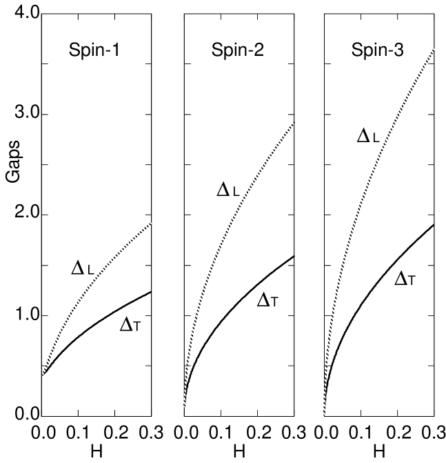
Figure 2: Transverse and longitudinal gaps in spin-1, 2, and 3 chains with the staggered field. We set $J=1$.

In Ref. Erco, , it has been confirmed that in the spin-1 chain, $m_{\rm s}^{z}$, $\Delta_{T}$ and $\Delta_{L}$ excellently agree with those determined from DMRG method within the weak-field regime ($H\ll J$). note0 Recalling again that the NLSM is a semiclassical approach, we can guess that the above quantities of the spin-2 and 3 chains, determined by the NLSM, are also consistent with their correct values at least in the regime $H\ll J$.

III Ladders and tubes

Based on the NLSM method for the single-chain problems in the preceding section, we investigate our targets, $N$-leg integer-spin ladders and tubes (1) in $T=0$.

III.1 No-field case

This subsection considers $N$-leg integer-spin ladders and tubes without external fields. (Here we remark that the 2-leg spin-1 case has already been analyzed by the NLSM, Sene a non-Abelian bosonization, Allen and the QMC simulation. Todo ) Following the method in Ref. Sene, , we treat the rung-coupling term as a perturbation on $N$ decoupled chains, each of which can be mapped to an NLSM. Namely, within the NLSM framework, we approximate it as follows:

$$J_{\perp}\sum_{l=1}^{\tilde{N}}\sum_{j}\vec{S}_{l,j}\cdot\vec{S}_{l+1,j} \to \frac{S^{2}J_{\perp}}{a}\sum_{l=1}^{\tilde{N}}\int dx\,\,\vec{n}_{l}\cdot\vec{n}_{l+1}$$ (16)

$$+\cdots,$$

where $\vec{n}_{l}$ is the AF fluctuation field of the $l$-th chain ($\vec{n}_{N+1}\equiv\vec{n}_{1}$). This prescription enables us to deal with any rung-coupling terms even including frustrations, although it would be valid only in the weak rung-coupling regime; $J\gg|J_{\perp}|$. However, as a price, we have to take into account $N$ constraints: $\vec{n}_{l}^{2}=1$ ($l=1,\dots,N$). (As well known, there is only one constraint in the standard NLSM method.) Here, as a crude approximation, we replace these constraints with an averaged one,

$$\sum_{l}\vec{n}_{l}^{2} = N.$$ (17)

We will discuss the validity of Eqs. (16) and (17) in the final part of this subsection. (As one will see there, we can predict that these two approximations are allowed in the any-leg weak-rung-coupling systems, at least within the qualitative level.) Under the approximations (16) and (17), the total action of ladders or tubes is described as

$$S_{\rm E}[\{\vec{n}_{l}\},\lambda] = \int d{\bf x}\,\Big{[}{}^{T}{\cal N}_{\alpha}{\bm{A}}{\cal N}_{\alpha}+iN\lambda\Big{]},$$ (18)

where the subscript ^T means transpose, ${\cal N}_{\alpha}={}^{T}(n_{1}^{\alpha},\dots,n_{N}^{\alpha})$, $\lambda$ is the auxiliary field for the constraint (17), and the $N\times N$ matrix $\bm{A}$ is defined as

$${\bm{A}} = \left(\begin{array}[]{cccccccc}a_{1}&a_{2}&&&a_{0}\\ a_{2}&a_{1}&\ddots&&\\ &\ddots&\ddots&\ddots&\\ &&\ddots&\ddots&a_{2}\\ a_{0}&&&a_{2}&a_{1}\\ \end{array}\right),$$ (19f)

$$a_{1} = -\frac{1}{2gc}\left(\partial_{\tau}^{2}+c^{2}\partial_{x}^{2}\right)-i\lambda,$$ (19g)

$$a_{2} = S^{2}J_{\perp}/(2a),$$ (19h)

where $a_{0}=0$ ($a_{2}$) for ladders (tubes). It is noteworthy that the action of an AF-rung ladder (an even-leg AF-rung tube) can be transformed to that of the ferromagnetic (FM)-rung ladder (the FM-rung tube) through the unitary transformation, $\vec{n}_{l={\rm even}}\to-\vec{n}_{l={\rm even}}$. Therefore, both AF- and FM-rung ladders (both even-leg AF- and FM-rung tubes) with the same leg number have the same low-energy excitation structure within the present scheme. Indeed, this property has been partially observed in a QMC study of the 2-leg spin-1 ladder with $|J_{\perp}|\ll J$. Todo On the other hand, we also emphasize that there are no unitary transformations connecting an odd-leg AF-rung (frustrated) tube and the FM-rung one.

Because the action (18) is quadratic in the fields $\vec{n}_{l}$ like the chain cases, we can integrate out $\vec{n}_{l}$ and derive the SPE for $\lambda$. After diagonalizing $\bm{A}$ (see Appendix A) and performing the Fourier transformations for $\vec{n}_{l}({\bf x})$, the action becomes

$$S_{\rm E} = \sum_{\bf k}\sum_{r}(\omega_{n}^{2}+\epsilon_{r}(k)^{2})\tilde{m}_{r}^{\alpha}({\bf k})^{*}\tilde{m}_{r}^{\alpha}({\bf k})$$ (20)

$$+iL\beta N\lambda_{\rm sp},\,\,\,\,\,\,\,\,$$

where

$$\epsilon_{r}(k) = c\sqrt{k^{2}+\xi_{r}^{-2}},$$ (21a)

$$\xi_{r}^{-2} \equiv \xi^{-2}+2J_{\perp}\cos k_{r}/(Ja^{2}),$$ (21b)

and $k_{r}=\frac{\pi r}{N+1}$ ($\frac{2\pi r}{N}$) and $r=1,\dots,N$ ($-[\frac{N}{2}]<r\leq[\frac{N}{2}]$) for ladders (tubes: $N\geq 3$). The symbol $[v]$ means the maximum integer $u$ satisfying $u\leq v$. The new field $\tilde{m}_{r}^{\alpha}({\bf k})$ is defined by $\tilde{m}_{r}^{\alpha}({\bf k})=U_{rl}\tilde{n}_{l}^{\alpha}({\bf k})$, where $U_{rl}$ is the unitary matrix diagonalizing $\bm{A}$. In the derivation of Eq. (20), we performed the replacement $\lambda\to\lambda_{\rm sp}$ (a constant), and assumed that $\lambda_{\rm sp}$ is purely imaginary. In tubes, $k_{r}$ means the wave number for the rung direction. Following the SPA prescription similar to that in Sec. II, we easily estimate the SPE, $\partial S_{\rm E}[\lambda_{\rm sp}]/\partial\lambda_{\rm sp}=0$, where $S_{\rm E}[\lambda]=-\ln(\int\prod_{l}{\cal D}\vec{n}_{l}e^{-S_{\rm E}[\{\vec{n}_{l}\},\lambda]})$, as follows:

$$\frac{3g}{2\pi}\sum_{r}\int_{0}^{\Lambda}\frac{dk}{\epsilon_{r}(k)}\coth\Big{(}\frac{\beta}{2}\epsilon_{r}(k)\Big{)} = N,$$ (22)

where we use the same cut off $\Lambda$ as that of chains. For $J_{\perp}=0$, Eq. (22) reduces to the SPE for chains (9).

The representation (20) tells us the following several low-energy properties of ladders and tubes. (i) One can interpret $\epsilon_{r}(k)$ as a spin-1 magnon dispersion. The band splitting $\epsilon(k)\to\epsilon_{r}(k)$ is due to the hybridization effect of the rung coupling. Each band $\epsilon_{r}(k)$ is triply degenerate correspondingly to $S^{z}=1$, $0$ and $-1$. (ii) The $3N$-band crossing occurs at $J_{\perp}=0$. Obtaining this level-crossing picture is an advantage of the NLSM approach. Sene Other methods, such as the QMC simulation Todo and the non-Abelian bosonization, Tsv ; Kita-Nomu ; Allen cannot derive it. (iii) In addition to the triple degeneracy of $S^{z}$, tubes (not ladders) have an extra degeneracy $\epsilon_{r}(k)=\epsilon_{-r}(k)$. Namely, in tubes, only two bands $\epsilon_{0}(k)$ and $\epsilon_{\frac{N}{2}}(k)$ are triply degenerate, while all other bands have a sixfold degeneracy. Here, note that the original tube (1) is invariant under reflection including (or $\pi$ rotation with respect to) the central axis of the cross section of tubes (Fig. 3). Because this operation causes $k_{r}\to-k_{r}$, we can conclude that the degeneracy $\epsilon_{r}(k)=\epsilon_{-r}(k)$ comes from the reflection symmetry and it must be a correct result independent of our approximation scheme. (iv) Noticing the contents of (i)-(iii) and the form of $\epsilon_{r}(k)$, we can show the band splitting as in Fig. 4. For any $r$, $\epsilon_{r}(k)$ has the minimum at $k=0$. Thus we define the gap of each band, $\Delta_{r}\equiv\epsilon_{r}(0)$. The true gap $\Delta_{\rm min}$ of the system would be the smallest among $\Delta_{r}$. For the nonfrustrated systems, $\Delta_{\rm min}$ is always carried by a triply degenerate band. Those of AF-rung ladders, FM-rung ladders, FM-rung tubes, and even-leg AF-rung tubes are given by $\Delta_{N}$, $\Delta_{1}$, $\Delta_{0}$, and $\Delta_{\frac{N}{2}}$, respectively. On the other hand, the gap of frustrated tubes is carried by a six-fold degenerate band with $\epsilon_{\frac{N-1}{2}}(k)=\epsilon_{-\frac{N-1}{2}}(k)$. This is a new even-odd property in the AF-rung spin tubes. This interesting phenomena can be intuitively understood as follows. The GS in all AF-rung tubes would tend to take a short-range Néel order along the rung. Therefore, we guess that the lowest excitations on such a GS are around the wave number $k_{r}=\pi$. Actually, those in nonfrustrated tubes always have $k_{r}=\pi$. However, the wave number $k_{r}=\pi$ can not be admitted in frustrated tubes. Instead, the lowest bands in $N$-leg frustrated tubes hence have $k_{r}=\pi\pm\frac{2\pi}{N}$, which is closest to $\pi$ in all the wave numbers. These bands are just sixfold degenerate. On the other hand, the lowest band in the FM-rung case always has $k_{r}=0$ because of the similar reason; FM-rung tubes tend to develop a FM short-range order along the rung. All the band with $k_{r}=0$ are not degenerate, except for the degeneracy of the spin-1 triplet.

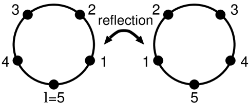
Figure 3: Cross section of the 5-leg tube and the reflecting operation for the rung direction.

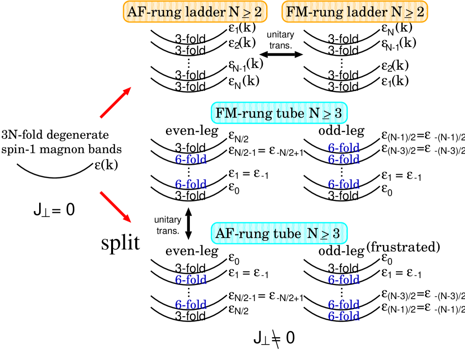
Figure 4: Band splitting induced by the rung coupling $J_{\perp}$. “Three- or sixfold” means the degree of the band degeneracy.

We investigate the low-energy excitations more quantitatively by solving the SPE (22). As we will see in Figs. 5-10, all ladders and tubes have a positive-$\xi_{r}$ solution, which means that all magnon bands $\epsilon_{r}(k)$ are well-defined. First, we discuss nonfrustrated systems. Figure 5 shows the rung-coupling and spin-magnitude dependence of gaps in 2-leg ladders. Figure 6 represents the rung-coupling dependence of gaps in $N$-leg spin-1 ladders. Moreover, Fig. 7 provides the lowest gap $\Delta_{\rm min}$ in $N$-leg spin-1 ladders and tubes. (Since the band structure of a nonfrustrated system with $J_{\perp}$ is equivalent to that of the system with $-J_{\perp}$ in the present scheme, the same result applies to the FM-rung ladders, and to even-leg AF-rung tubes.) The former two figures indicate that the rung coupling induces rapid rises of bands except for the lowest bands. It supports the known result that the standard NLSM approach for nonfrustrated systems, Sier ; Dell which extracts only the lowest bands, captures the low-energy physics in $|J_{\perp}|\sim J$. Figure 6 shows that the increase of $N$ gradually enlarges splitting-magnon-band width. One finds from Figs. 5 and 7 that the more $N$ or $S$ increase, the larger the decreasing speed of gaps $\Delta_{\rm min}$ becomes around the decoupling point $J_{\perp}=0$. Particularly, in Fig. 5, it is remarkable that once one attaches an awfully weak rung coupling for a ladder with $S>1$, the gap $\Delta_{\rm min}$ sharply approaches zero. For example, when we set $(J,J_{\perp},T)=(1,0.05,0)$, the SPA predicts $(\Delta_{\rm min},\frac{\Delta_{\rm min}}{\Delta})=(0.268,0.653)$ for $S=1$, $(0.0143,0.160)$ for $S=2$, and $(0.000459,0.0458)$ for $S=3$ ($\Delta$ is the Haldane gap of single chains in Table 1). These gap reductions are naturally expected from the consideration that the growths of $S$ and $N$ help the GS (a massive spin-liquid state) be close to a Néel state, which has a massless Nambu-Goldstone mode.

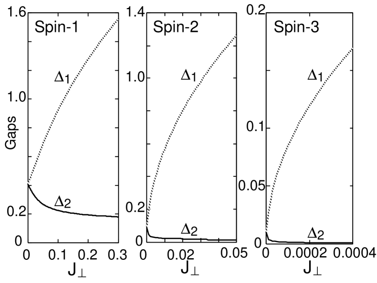
Figure 5: Gaps $\Delta_{1}$ and $\Delta_{2}=\Delta_{\rm min}$ in 2-leg AF-rung spin-1, -2, or -3 ladders with $J=1$.

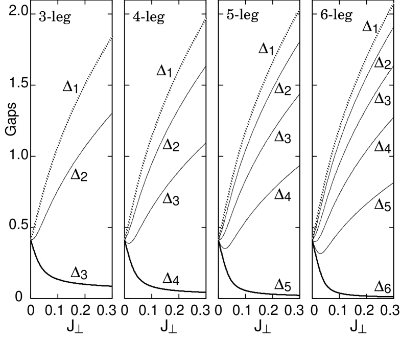
Figure 6: All band gaps $\Delta_{r}$ in $N$-leg AF-rung spin-1 ladders with $J=1$.

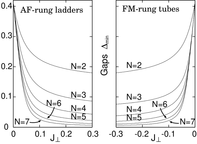
Figure 7: Lowest magnon gaps $\Delta_{\rm min}$ in $N$-leg AF-rung spin-1 ladders and FM-rung tubes (non-frustrated systems) with $J=1$. The gap-reduction speed of the $N$-leg tube is larger a little than that of the ladder. The 2-leg “tube” means the 2-leg ladder.

We next focus on the frustrated spin tubes. Figure 8 is the gap structures of AF-rung spin-1 tubes. The panel (a) shows that gap reductions of frustrated (odd-leg) tubes are considerably slower than those of even-leg tubes. It must reflect that the rung frustration obstructs the rise of the AF short-range order unlike in the nonfrustrated systems. While, similarly to nonfrustrated systems, the growth of $N$ prompts the gap reduction in the frustrated tubes. It would be a relaxation effect of the frustration. We see from the panels (b) that all magnon bands, except for lowest one, quickly rise together with increasing $J_{\perp}$ even in frustrated tubes. This may suggest the possibility to construct an effective theory for frustrated tubes, which includes only lowest sixfold degenerate bands.

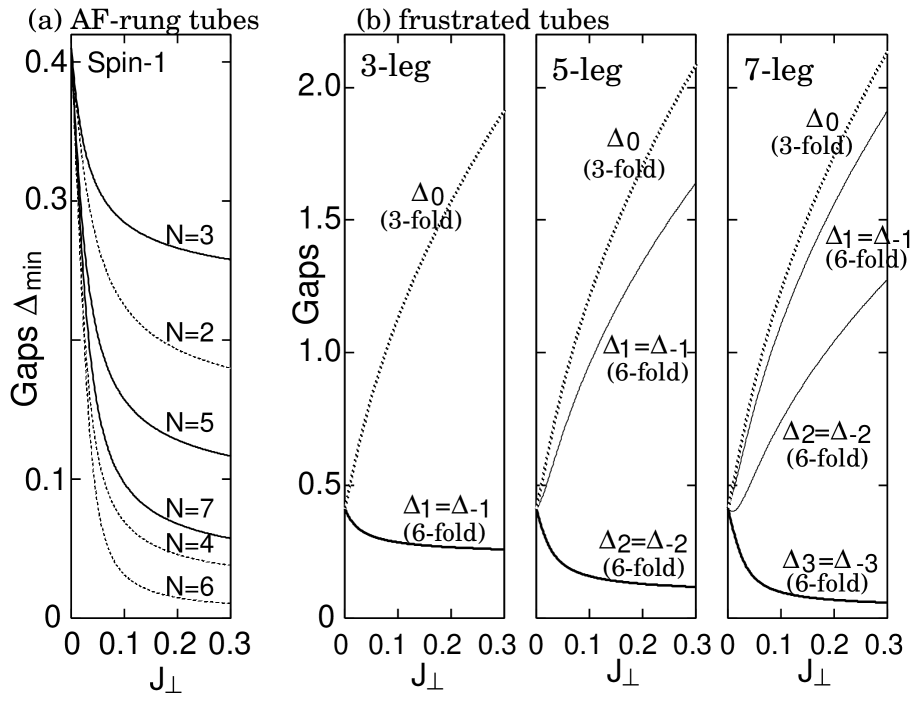
Figure 8: Lowest magnon gaps $\Delta_{\rm min}$ and band gaps $\Delta_{r}$ in $N$-leg AF-rung spin-1 tubes with $J=1$.

Finally, we discuss the validity of our strategy in this subsection. In order to investigate the integer-spin ladders and tubes, we took approximations (16) and (17). First, we consider the validity of Eq. (17). If we adopt the original constraint $\vec{n}_{l}^{2}=1$ ($l=1,\dots,N$) instead of the averaged one (17), the action corresponding to the model (1) is given by

$$S_{\text{E}}^{\prime}[\{\vec{n}_{l}\},\{\lambda_{l}\}]=\int\,d{\bf x}\Big{\{}\sum_{l=1}^{N}\Big{[}\vec{n}_{l}\Big{(}-\frac{1}{2gc}\left(\partial_{\tau}^{2}+c^{2}\partial_{x}^{2}\right)$$

$$-i\lambda_{l}\Big{)}\vec{n}_{l}+i\lambda_{l}\Big{]}+\frac{S^{2}J_{\perp}}{a}\sum_{l=1}^{\tilde{N}}\vec{n}_{l}\cdot\vec{n}_{l+1}\Big{\}},\,\,\,\,\,\,\,\,$$ (23)

where $\lambda_{l}$ is the auxiliary field for the constraint $\vec{n}_{l}^{2}=1$. At least for the 2-leg ladder system, the SPEs for the original constraint $\vec{n}_{1}^{2}=\vec{n}_{2}^{2}=1$ turn out to be identical with that for the averaged one. Sene The deviation between original and averaged constraints could appear in 3-leg or higher-leg systems within the SPA. Actually, one can easily check that the SPEs for the original and averaged constraints provide different solutions in the 3-leg ladder. Therefore, averaging (17) is expected to be invalid for large-$N$ systems. Here, notice that the action (III.1) is invariant under the transformation $\vec{n}_{l}\to\vec{n}_{l+{\cal Q}}$ and $\lambda_{l}\to\lambda_{l+{\cal Q}}$ [${\cal Q}\in\mathbb{Z}$] ($\vec{n}_{l}\to\vec{n}_{N+1-l}$ and $\lambda_{l}\to\lambda_{N+1-l}$) in the tube (ladder) systems. These transformations of course correspond to the translational operation along the rung in tubes ($\vec{S}_{l,j}\to\vec{S}_{l+{\cal Q},j}$) and reflection around the central axis along the chain in ladders ($\vec{S}_{l,j}\to\vec{S}_{N+1-l,j}$), respectively. Let us discuss the form of the SPEs, using these symmetries. Each original SPE is written as $\partial S^{\prime}_{\rm{E}}[\{\lambda_{m}\}]/\partial\lambda_{l}\propto\langle\vec{n}_{l}^{2}-1\rangle=0$, where $S^{\prime}[\{\lambda_{m}\}]=-\ln(\int\prod_{m}{\cal D}\vec{n}_{m}e^{-S_{\text{E}}^{\prime}[\{\vec{n}_{m}\},\{\lambda_{m}\}]})$. The expectation value $\langle\vec{n}_{l}^{2}\rangle$ is a function of $\{\lambda_{m}\}$; $\langle\vec{n}_{l}^{2}\rangle=f(\lambda_{1},\cdots,\lambda_{N})$. In the tube systems, these facts and the above symmetry of the action (III.1) lead to the identity $1=\langle\vec{n}_{l}^{2}\rangle=f(\lambda_{1},\cdots,\lambda_{N})=\langle\vec{n}_{l+1}^{2}\rangle=f(\lambda_{2},\cdots,\lambda_{N},\lambda_{1})=\cdots$. Therefore, we find that $\partial S^{\prime}_{\rm{E}}[\{\lambda_{m}\}]/\partial\lambda_{l}|_{\lambda_{1}=\cdots=\lambda_{N}}$ is independent of all the chain indices $l$ in tubes. On the other hand, in tubes, the SPE for the averaged constraint concerns those for the original ones as follows:

$$0=\frac{\partial S_{\rm{E}}[\lambda]}{\partial\lambda} = \sum_{l=1}^{N}\frac{\partial S_{\rm{E}}^{\prime}[\{\lambda_{m}\}]}{\partial\lambda_{l}}\Big{|}_{\lambda_{1}=\cdots=\lambda_{N}=\lambda}$$ (24)

$$= N\frac{\partial S_{\rm{E}}^{\prime}[\{\lambda_{m}\}]}{\partial\lambda_{1}}\Big{|}_{\lambda_{1}=\cdots=\lambda_{N}=\lambda},$$

where the final equal sign is thanks to the above property of the function $f$. Because we have already known that $\partial S_{\rm{E}}[\lambda]/\partial\lambda=0$ has a physically suitable solution $\lambda_{\rm{sp}}$, Eq. (24) indicates that the original SPEs in tubes can take the same solution, $\lambda_{1}=\cdots=\lambda_{N}=\lambda_{\rm{sp}}$. Thus, the averaging of the constraints, Eq. (17), should be valid on the symmetric solutions of the original SPEs, $\lambda_{1}=\cdots=\lambda_{N}$, although other possible solutions would not be covered. Meanwhile, in ladder systems, the similar argument can not lead to the validity of Eq. (17). If the effective theory (III.1) for ladders possesses the reflection symmetry ($\vec{S}_{l,j}\to\vec{S}_{N+1-l,j}$), the original SPEs should have a solution with $\lambda_{l}=\lambda_{N+1-l}$. This solution does not contradict the symmetric one. Therefore, we expect that the averaging (17) is admitted even in ladders.

Subsequently, we discuss the perturbative treatment of the rung coupling (16). As mentioned before, the approximation (16) would be justified only in the weak rung-coupling regime $|J_{\perp}|\ll J$. As we see from Figs. 5-8, the present scheme always predicts that the gap $\Delta_{\rm min}$ monotonically decreases with $|J_{\perp}|$ increasing in all systems. However, it has been known, from the QMC simulation, Todo that in the 2-leg spin-1 AF-rung ladder, the gap reaches its minimum value at a finite $J_{\perp}$, and then grows and approaches the gap for the 2-spin problem in the single rung with increasing $J_{\perp}$. (The simulation also shows that the gap monotonically decreases for FM-rung side.) In addition, the standard NLSM method for nonfrustrated systems, Sier ; Dell ; Sene which is reliable for the case $|J_{\perp}|\sim J$, shows that the gap is a monotonically increasing function of $J_{\perp}$ in all the AF-rung cases. These gap growths cannot be explained in our weak rung-coupling framework. (Inversely, it also means that the standard NLSM approach breaks down in the weak rung-coupling regime.) Figure 9 displays gaps $\Delta_{\rm min}$ of spin-1 ladders and tubes with a few leg numbers, which are determined from the SPA and the QMC method (note that the QMC method cannot be applicable for the frustrated tubes doe to the negative-sign problem). As expected, the SPA gap is semiquantitatively identical to the QMC one within the sufficiently weak rung-coupling regime $|J_{\perp}|\lesssim 0.05\times J$, outside which the deviation between SPA and QMC gaps becomes clear. The good agreement between the SPA and QMC methods is observed in 2, 3, and 4-leg systems. It encourages and allows us to apply the present SPA scheme to large-$N$ systems. The SPA gap is always larger than the QMC one in the region $|J_{\perp}|\gtrsim 0.05\times J$. It might be because the SPA does not take into account the quantum fluctuation effects enough. In Fig. 10, we draw the spin-spin correlation lengths of small-$N$ systems, which are determined by the SPA and the QMC methods. There, we define the SPA correlation length as $\xi_{\rm corr}\equiv c\Delta_{\rm min}^{-1}$. Since our scheme optimizes the gaps and not the correlation lengths, the deviation of the SPA and QMC data already emerges at the starting point $J_{\perp}=0$. However, like the gap, the behavior of the SPA correlation lengths is similar to that of the QMC ones within $|J_{\perp}|\lesssim 0.05\times J$.

We believe that our results are qualitatively correct in all ladders and tubes with a weak rung coupling, and in particular, the predicted band structures in Fig. 4 are true. The band degeneracy is strongly protected by the symmetry argument. Like the final statements in Sec. II.1, one can imagine several modifications of approximations (16) and (17).

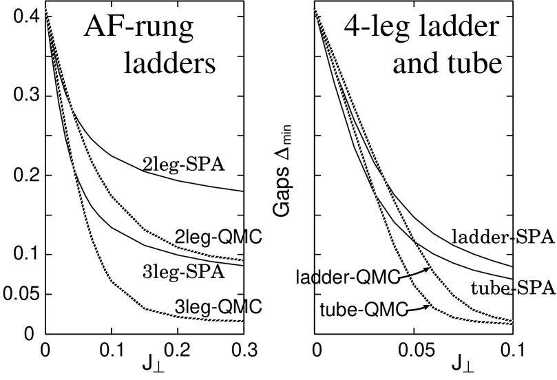
Figure 9: Gaps $\Delta_{\rm min}$ of spin-1 ladders and tubes with $J=1$. Marks “SPA” and “QMC” mean “derived by the SPA” and “derived by the QMC simulation” respectively. The QMC data, which all achieve their thermodynamic-limit values, are calculated by Munehisa Matsumoto. MMcom The method of determining the gap and the correlation length in the QMC simulation is, for example, explained in Refs. Todo-Kato, adn Todo, .

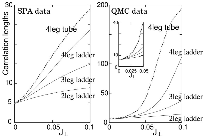
Figure 10: Spin correlation lengths in spin-1 ladders and tubes determined by the SPA or the QMC simulation. The QMC data is provided by Munehisa Matsumoto. MMcom

III.2 $[0,0]$-field case

In this subsection, we investigate the ladders and tubes with the uniform Zeeman term (2a). To this end, one first had better notice the following general aspects in 1D spin systems. (i) The uniform field always splits triply degenerate spin-1 magnon states into $S^{z}=1$, $0$ and $-1$ states. (ii) When a magnon band crosses the zero energy and the magnon condensation occurs in a 1D U(1)-symmetric spin system, the GS is usually regarded as a $c=1$ one-component TLL. Masa ; S-A ; Tsv ; Aff-magcond ; Aff-bose ; S-T ; Kon ; Fath The combination of these statements and the band structures in Fig. 4 leads to the conjecture that as a sufficiently strong uniform field is applied, nonfrustrated systems enter in a standard one-component TLL phase ($c=1$), whereas the GSs of frustrated tubes become a two-component TLL ($c=1+1$). This is another new even-odd property in AF-rung tubes.

However, as multimagnon modes are condensed simultaneously, interactions among the resulting massless excitations (TLLs) can be present in general. They could induce the hybridizations and gaps in a part of the massless modes. [For example, on the $c=1+1$ critical GS of two independent spin-$\frac{1}{2}$ (or spin-1) AF chains with a uniform field, Masa ; Cabra ; Selton ; Fu-Zh a rung coupling brings the hybridization of massless modes. As a result, a massless mode becomes gapful and only the other one remains being massless.] While, all magnon excitations have to possess a wave number $k_{r}$ in the (frustrated) tubes, due to the translational symmetry along the rung. Moreover, the tubes also have the reflection symmetry (Fig. 3). Therefore, we expect that when the lowest doubly degenerate magnons are condensed in frustrated tubes, these two symmetries strongly restrict possible interactions and hybridizations between the low-energy excitations. Consequently, it would be natural that two kinds of massless excitations are present after the lowest two magnon bands are condensed. It has been suggested in Ref. Cit, that a strong uniform field brings a $c=1+1$ phase in the 3-leg AF-rung “spin-$\frac{1}{2}$” tube. (Note that this massless phase of the spin-$\frac{1}{2}$ tube is located just under the saturated state. While, the massless phase in the integer-spin tube, expected here, appears just when an infinitesimal magnetization occurs.) Therefore, the emergence of a GS with two bosonic massless modes might be universal for odd-leg AF-rung (frustrated) spin tubes with any spin magnitudes.

We investigate the above expectation of the $c=1+1$ phase in more detail, below. First, we demonstrate that our NLSM plus SPA method for ladders and tubes can reproduce the Zeeman splitting in Sec. III.2.1. Subsequently, in Secs. III.2.2 and III.2.3, we discuss the magnon condensed state in frustrated tubes using a heuristic bosonization method. The discussion there takes into account the translational symmetry along the rung and the reflection one more carefully. The results further support the presence of the $c=1+1$ state.

III.2.1 Zeeman splitting in ladders and tubes

From Eqs. (13) and (18), we can represent the Euclidean action of the [0,0]-field case, in the Fourier space, as follows:

$$S_{\rm E}^{[0,0]}[\{\vec{n}_{l}\},\lambda_{\rm sp}] = \sum_{\bf k}\Big{[}\tilde{\cal N}_{\perp}^{\dagger}\tilde{\bm{A}}_{\perp}\tilde{\cal N}_{\perp}$$ (25)

$$+\tilde{\cal N}_{z}^{\dagger}\tilde{\bm{A}}_{z}\tilde{\cal N}_{z}\Big{]}+iN\beta L\lambda_{\rm sp},$$

where the mark ^† means Hermitian conjugate, $\tilde{\cal N}_{\alpha}({\bf k})=(\tilde{n}_{1}^{\alpha}({\bf k}),\dots,\tilde{n}_{N}^{\alpha}({\bf k}))$, $\tilde{\cal N}_{\perp}({\bf k})=({}^{T}\tilde{\cal N}_{x}({\bf k}),{}^{T}\tilde{\cal N}_{y}({\bf k}))$. The $2N\times 2N$ matrix $\tilde{\bm{A}}_{\perp}$ and $N\times N$ one $\tilde{\bm{A}}_{z}$ are defined by

$$\tilde{\bm{A}}_{\perp}({\bf k}) = \left(\begin{array}[]{ccc}{\bm{A}}_{\bf k}&{\bm{E}}_{\omega_{n}}\\ -{\bm{E}}_{\omega_{n}}&{\bm{A}}_{\bf k}\end{array}\right),$$ (26c)

$${\bm{A}}_{\bf k} = \left(\begin{array}[]{cccccc}\tilde{a}_{1}&\tilde{a}_{2}&&&\tilde{a}_{0}\\ \tilde{a}_{2}&\tilde{a}_{1}&\ddots&&\\ &\ddots&\ddots&\ddots&\\ &&\ddots&\ddots&\tilde{a}_{2}\\ \tilde{a}_{0}&&&\tilde{a}_{2}&\tilde{a}_{1}\end{array}\right),$$ (26i)

$${\bm{E}}_{\omega_{n}} = -\frac{H\omega_{n}}{gc}\hat{\bm{1}},$$ (26j)

$$\tilde{\bm{A}}_{z}({\bf k}) = {\bm{A}}_{\bf k}+\frac{H^{2}}{2gc}\hat{\bm{1}},$$ (26k)

where $\tilde{a}_{1}=(\omega_{n}^{2}+\epsilon(k)^{2})/(2gc)$, $\tilde{a}_{2}=a_{2}$, $\tilde{a}_{0}=0$ [$\tilde{a}_{2}$] for ladders [tubes], and $\hat{\bm{1}}$ is an $N\times N$ unit matrix. We stress that $\tilde{\bm{A}}_{\perp}$ is not Hermite but normal ($\tilde{\bm{A}}_{\perp}^{\dagger}\tilde{\bm{A}}_{\perp}=\tilde{\bm{A}}_{\perp}\tilde{\bm{A}}_{\perp}^{\dagger}$), so it can be diagonalized by a unitary matrix (hence, we do not need to consider the Jacobian generated from the diagonalization in the path-integral formalism). From Eqs. (81)-(86), the eigenvalues of $\tilde{\bm{A}}_{\perp}$ [$\tilde{\bm{A}}_{z}$] are $A_{r}^{\pm}=(\omega_{n}^{2}+\epsilon_{r}(k)^{2}\pm 2iH\omega_{n})/(2gc)$ [$A_{r}^{z}=(\omega_{n}^{2}+\epsilon_{r}(k)^{2}+H^{2})/(2gc)$]. Using these, we can integrate out $\vec{n}_{l}$ in $Z$ and derive the SPE,

$$\frac{gc}{2\pi}\sum_{r}\int_{0}^{\Lambda}\frac{dk}{\epsilon_{r}^{0}(k)}\sum_{z=0,+,-}\coth\Big{(}\frac{\beta}{2}\epsilon_{r}^{z}(k)\Big{)} = N,$$ (27)

where $\epsilon_{r}^{0}(k)=c\sqrt{k^{2}+\xi_{r}^{-2}+H^{2}/c^{2}}$ and $\epsilon_{r}^{\pm}(k)=\epsilon_{r}^{0}(k)\mp H$. The quantities $\epsilon_{r}^{0,+,-}(k)$ can be considered as the magnon dispersions. The comparison between Eqs. (27) and (22) elucidates the relation $\xi_{r}(H=0)^{-2}=\xi_{r}(H)^{-2}+H^{2}/c^{2}$ at $T=0$. Thus, one can see that new dispersions $\epsilon_{r}^{z}(k)$ restore the Zeeman splitting at $T=0$. The magnons with $\epsilon_{r}^{0}(k)$, $\epsilon_{r}^{+}(k)$ and $\epsilon_{r}^{-}(k)$ take $S^{z}=0$, $1$ and $-1$, respectively.

Strictly speaking, the above SPA cannot handle the strong-field case ($H\sim J$), where some magnons are condensed, since the magnon condensation and the finite uniform magnetization are not taken into account in the Haldane mapping (4). However, as will be explained below, under certain approximations, the above consideration can be extended to the situation where the magnons are condensed.

III.2.2 Magnon condensed state in frustrated tubes

Referring the arguments in Refs. Aff-magcond, and Kon, , we try to construct the effective theory for the magnon condensed state in frustrated tubes. After integrating out the magnon fields except for the degenerate lowest ones in the action (25), the effective action would be given as

$$S_{\rm{eff}}[\vec{m}_{\pm p}] = \sum_{q=\pm p}\int d{\bf x}\Big{\{}\frac{1}{2gc}\Big{[}(\partial_{\tau}\vec{m}_{q})^{2}+c^{2}(\partial_{x}\vec{m}_{q})^{2}\Big{]}$$ (28)

$$-\frac{i}{gc}\vec{H}\cdot(\vec{m}_{q}\times\dot{\vec{m}}_{q})+V(\vec{m}_{q})\Big{\}},$$

where $p=\frac{N-1}{2}$ ($k_{p}=\frac{N-1}{N}\pi$) and

$$\vec{m}_{r}({\bf x}) = U_{rl}\vec{n}_{l}({\bf x})=\sqrt{\frac{2}{N}}\sum_{l=1}^{N}\sin(k_{r}l+\pi/4)\vec{n}_{l},\,\,\,\,\,\,\,\,$$ (29a)

$$V(\vec{m}_{q}) = \frac{\Delta_{q}^{2}-H^{2}}{2gc}\vec{m}_{q}^{2}+\frac{H^{2}}{2gc}(m_{q}^{z})^{2}+u|\vec{m}_{q}|^{4}.$$ (29b)

In the potential $V(\vec{m}_{q})$, $\Delta_{q}=\Delta_{\rm{min}}$ ($\Delta_{\rm{min}}$ is defined in the no-field case), $c\xi_{q}^{-1}=\frac{\Delta_{q}^{2}-H^{2}}{2gc}$, and we introduced the biquadratic term $u|\vec{m}_{q}|^{4}$ to ensure the stability of the magnon condensed state [one can interpret that it originates from the large-$N$ expansion for the O($N$) NLSM]. We perform the Ginzburg-Landau (GL) analysis (i.e., a mean-field theory) for the action (28). The minimum of the GL potential $V(\vec{m}_{q})$ is at $\vec{m}_{q}=0$ in the weak uniform-field regime $H<\Delta_{q}$. On the other hand, as $H$ exceeds $\Delta_{q}$, the minimum is located in the field configuration,

$$(m_{q}^{x})^{2}+(m_{q}^{y})^{2}=\frac{H^{2}-\Delta_{q}^{2}}{4ugc}\equiv\bar{m}^{2}, m^{z}=0.$$ (30)

Namely, $H=\Delta_{q}$ is just the critical point between the condensed phase with a finite uniform magnetization and the noncondensed phase, within the GL analysis. For the condensed case $H>\Delta_{q}$, let us introduce the new field parameterization,

$$m_{q}^{\pm}\equiv m_{q}^{x}\pm im_{q}^{y} = (\bar{m}_{q}+\bar{m})e^{\pm i\sqrt{\pi}\theta_{q}}.$$ (31)

Substituting Eq. (31) in the action (28), we obtain

$$S_{\rm{eff}} = \sum_{q=\pm p}\int d{\bf x}\Big{\{}\frac{1}{2gc}\Big{[}(\partial_{\tau}m_{q}^{z})^{2}+c^{2}(\partial_{x}m_{q}^{z})^{2}\Big{]}$$ (32)

$$+\frac{1}{2gc}\Big{[}(\partial_{\tau}\bar{m}_{q})^{2}+c^{2}(\partial_{x}\bar{m}_{q})^{2}\Big{]}$$

$$+\frac{H^{2}}{2gc}(m_{q}^{z})^{2}+\frac{H^{2}-\Delta_{q}^{2}}{gc}\bar{m}_{q}^{2}$$

$$-i\frac{\sqrt{\pi}H}{gc}(2\bar{m}\bar{m}_{q}+\bar{m}^{2})\partial_{\tau}\theta_{q}$$

$$+\frac{\pi\bar{m}^{2}}{2gc}\Big{[}(\partial_{\tau}\theta_{q})^{2}+c^{2}(\partial_{x}\theta_{q})^{2}\Big{]}+\dots\Big{\}},$$

up to the quadratic order of the fields. The action (32) indicates that fields $m_{q}^{z}$ and $\bar{m}_{q}$ are massive, and it means that the low-energy limit of the magnon condensed state is described by the two phase fields $\theta_{q=\pm p}$. If one integrates out the massive fields neglecting the third or higher derivatives of all fields in the action (32), the resultant effective Euclidean Lagrangian density is

$${\cal L}_{\rm{E}}(\theta_{p},\theta_{-p}) = \sum_{q=\pm p}\frac{K}{2v}\Big{[}(\partial_{\tau}\theta_{q})^{2}+v^{2}(\partial_{x}\theta_{q})^{2}\Big{]}$$ (33)

$$-ih_{1}\partial_{\tau}\theta_{q},\,\,\,\,$$

where $K=\frac{\pi\bar{m}^{2}}{g}\sqrt{h_{2}}$, $v=c/\sqrt{h_{2}}$, $h_{1}=\sqrt{\pi}H\bar{m}^{2}/(gc)$, and $h_{2}=(3H^{2}-\Delta_{q}^{2})/(H^{2}-\Delta_{q}^{2})$. This is just the Lagrangian density for a two-component TLL: CFT ; Gogo $K$ and $v$ correspond to the TLL parameter and the Fermi velocity, respectively. These two quantities are renormalized, from their values of the GL theory, by the interactions neglected here (we will discuss the effects of such interactions below). It has been known that in the vicinity of the lower or upper critical fields, the TLL parameter for a gapless AF spin chain preserving the $z$ component of the total spin is generally approximated as unity corresponding to the free fermion. Aff-magcond ; Kon ; Hal2 Under the assumption that this property also holds in tubes, $K$ in Eq. (33) is close to unity as $H\to\Delta_{q}+0$. Here, imitating $\vec{m}_{r}=U_{rl}\vec{n}_{l}$, we define the Fourier transformation of the spin operator as $\vec{T}_{r}\equiv U_{rl}\vec{S}_{l,j}\approx\vec{T}_{r,\rm{u}}+(-1)^{j}\vec{T}_{r,\rm{st}}$. Equations (31), (6), and (12) serve

$$T_{0,\rm{u}}^{z} = \frac{1}{\sqrt{N}}\sum_{j}\frac{i}{4J}(\vec{n}_{j}\times\dot{\vec{n}}_{j})^{z}+\frac{H}{4J}[1-(n_{j}^{z})^{2}]$$ (34a)

$$= \frac{1}{\sqrt{N}}\sum_{r}\frac{i}{4J}(\vec{m}_{r}\times\dot{\vec{m}}_{r})^{z}+\dots$$

$$\approx \frac{1}{\sqrt{N}}\Big{[}\frac{i\bar{m}^{2}}{4J}(\partial_{\tau}\theta_{p}+\partial_{\tau}\theta_{-p})+\dots\Big{]},$$

$$T_{q,\rm{st}}^{+} \approx (\bar{m}_{q}+\bar{m})e^{i\sqrt{\pi}\theta_{q}}+\dots,$$ (34b)

where the latter equation suggests that the radius of $\theta_{q}$ is $1/\sqrt{\pi}$, and it also means that the radius of the dual field $\phi_{q}$ is $1/\sqrt{4\pi}$ in our notation: Gogo the equal-time commutation relation between $\theta_{q}$ and $\phi_{q}$ is defined as $[\phi_{q}(x),\theta_{q}(y)]=i\Theta_{\rm s}(y-x)$, Shank ; Delft where $\Theta_{\rm s}$ is the Heaviside’s step function. We expect that $\partial_{\tau}\theta_{q}$ ($e^{i\sqrt{\pi}\theta_{q}}$) in Eq. (34) is the most relevant bosonic term in the effective representation of $T_{0,\rm{u}}^{z}$ ($T_{q,\rm{st}}^{+}$). However, it is difficult to determine the forms of second relevant or more irrelevant terms within only the above NLSM plus GL analysis.

In order to examine a more proper bosonic representation of $\vec{T}_{r}$, let us once review the low-energy physics of a spin-1 AF chain with a uniform field. In addition to the NLSM approach in Sec. II, there is another low-energy effective theory for the spin-1 AF chains. The latter approximates the spin-1 chain without external fields as three copies of massive real fermions, each of which is equivalent to an off-critical transverse Ising chain. Masa ; Tsv ; Allen ; Kita-Nomu In this scheme, the spin operator is written as

$$S_{j}^{\alpha} \approx S_{\rm{u}}^{\alpha}+(-1)^{j}S_{\rm{st}}^{\alpha},\,\,\,\,(\alpha=1,2,3\,\rm{or}\,x,y,z),\,\,\,\,$$

$$S_{\rm{u}}^{\alpha}/a = -i(\xi_{L}^{\alpha+1}\xi_{L}^{\alpha+2}+\xi_{R}^{\alpha+1}\xi_{R}^{\alpha+2}),$$

$$S_{\rm{st}}^{\alpha}/a = C_{\rm{st}}\sigma_{\alpha}\mu_{\alpha+1}\mu_{\alpha+2},\,\,\,\,(\alpha+3=\alpha),$$ (35)

where $\xi_{L(R)}^{\alpha}$ is the left (right) mover of the $\alpha$th real fermion, $\sigma_{\alpha}$ ($\mu_{\alpha}$) stands for the order (disorder) field in the $\alpha$-th Ising system, and $C_{\rm{st}}$ is a nonuniversal constant. The GS in the fermion picture corresponds to the disorder phase in the Ising picture: $\langle\mu_{\alpha}\rangle\neq 0$. When the uniform field exceeds the lower critical value, the low-energy physics is governed by a TLL with a scalar boson $\phi$ and its dual $\theta$. In this case, the representation of the spin operator (III.2.2) should be changed by using these two fields. Equation (III.2.2) and the known results of the 2-leg spin-$\frac{1}{2}$ AF ladder with a uniform field Selton ; Fu-Zh provide a desirable representation,

$$\frac{S_{\rm{u}}^{z}}{a} \approx \frac{\partial_{x}\phi}{\sqrt{\pi}}+\frac{M_{u}}{a}+C_{1}\cos\Big{[}\sqrt{4\pi}\phi+\frac{2\pi M_{u}x}{a}\Big{]},\,\,\,\,\,\,\,\,$$ (36a)

$$\frac{S_{\rm{st}}^{z}}{a} \approx C_{2}\sigma_{3}\cos\Big{[}\sqrt{\pi}\phi+\frac{\pi M_{u}x}{a}\Big{]},$$ (36b)

$$\frac{S_{\rm{st}}^{+}}{a} \approx C_{3}\mu_{3}e^{i\sqrt{\pi}\theta}\Big{\{}1$$ (36c)

$$+C_{4}\sin\Big{[}\sqrt{4\pi}\phi+\frac{2\pi M_{u}x}{a}\Big{]}\Big{\}},\,\,\,\,\,\,\,\,\,\,$$

where $M_{u}=\langle S_{j}^{z}\rangle$, and $C_{1\text{-}4}$ are a constant. The third fermion system is still massive (it corresponds to $\langle\mu_{3}\rangle\neq 0$) and the fermion $\xi_{L,R}^{3}$ stands for the magnon with $S^{z}=0$. The formula (36) is valid in $M_{u}\ll 1$. Fu-Zh Equation (36c) means that the radius of $\theta$ is $1/\sqrt{\pi}$. While, Eq. (36b) also suggests that the radius of $\phi$ is the same value, $1/\sqrt{\pi}$. This apparently contradicts the framework of the standard TLL theory. Actually, if we allow the presence of both $e^{i\sqrt{\pi}\theta}$ and $e^{i\sqrt{\pi}\phi}$, the commutation relation between these two is nonlocal: $e^{i\sqrt{\pi}\phi(x)}e^{i\sqrt{\pi}\theta(y)}=e^{-\pi[\phi(x),\theta(y)]}e^{i\sqrt{\pi}\theta(y)}e^{i\sqrt{\pi}\phi(x)}={\rm sgn}(y-x)e^{i\sqrt{\pi}\theta(y)}e^{i\sqrt{\pi}\phi(x)}$ $(x\neq y)$, where ${\rm sgn}(y-x)$ is the sign function. The nonlocal property is inconsistent with the fact that the original spin-1 operators are mutually local (i.e., two spins on different sites commute with each other). However, observing Eq. (36) carefully, one can find that the nonlocality between $\sigma_{3}$ and $\mu_{3}$ and that between $\cos(\sqrt{\pi}\phi+\pi M_{u}x/a)$ and $e^{i\sqrt{\pi}\theta}$ cooperatively restore the locality among the spin operators $S_{j}^{z}$ and $S_{k}^{\pm}$. Therefore, we believe that the formula (36) is valid and the radius of $\theta$ ($\phi$) may be defined as $1/\sqrt{\pi}$ ($1/\sqrt{4\pi}$). Here, further notice that the effective Hamiltonian in the spin-$1$ chain has to be constructed by the sum of terms being locally related with each other, because the original chain is a locally interacting system. This statement must hold in the effective theories of the ladders and tubes (1).

Now, we go back to the frustrated tubes. Following Refs. Aff-magcond, and Kon, , one can see that the $\vec{m}_{p}$ (or $\vec{m}_{-p}$) part of the effective action (28) [or (32)] is the same form as the effective one for the spin-1 chain with a uniform field. Moreover, the bosonic representation (34) is very similar to that of the spin-1 chain, Eq. (36). From these facts, it is expected that Eq. (36) helps us improve the imperfect formula (34). We propose the following new bosonic representation of $\vec{T}_{r}$:

$$\sqrt{N}T_{0,\rm{u}}^{z} \approx \frac{a}{\sqrt{\pi}}(\partial_{x}\phi_{p}+\partial_{x}\phi_{-p})+2M_{t}$$ (37a)

$$+C_{t1}\Big{\{}\cos\Big{[}\sqrt{4\pi}\phi_{p}+\frac{2\pi M_{t}x}{a}\Big{]}$$

$$+\cos\Big{[}\sqrt{4\pi}\phi_{-p}+\frac{2\pi M_{t}x}{a}\Big{]}\Big{\}},$$

$$T_{q,\rm{st}}^{z} \approx C_{t2}\cos\Big{[}\sqrt{\pi}\phi_{q}+\frac{\pi M_{t}x}{a}\Big{]},$$ (37b)

$$T_{q,\rm{st}}^{+} \approx C_{t3}e^{i\sqrt{\pi}\theta_{q}}\Big{\{}1$$ (37c)

$$+C_{t4}\sin\Big{[}\sqrt{4\pi}\phi_{q}+\frac{2\pi M_{t}x}{a}\Big{]}\Big{\}},\,\,\,\,\,\,\,\,\,\,\,$$

where $\phi_{q}$ is the dual of $\theta_{q}$, and $C_{t1\text{-}t4}$ are a constant. The first term in Eq. (37a) would be acceptable from the real-time operator identity $\frac{1}{v}\partial_{t}\theta_{q}=\partial_{x}\phi_{q}$. The parameter $M_{t}$ can be fixed by the magnetization per site $\langle S_{l,j}^{z}\rangle=2M_{t}/N$. (Determining the correct value of $M_{t}$ is difficult within the GL theory.) To preserve the locality among the spin operators $T_{q}^{\alpha}$, we should regard that $C_{t2}$ and $C_{t3}$ contain massive fields such as $\sigma_{3}$ and $\mu_{3}$ in Eq. (36). However, since we actually cannot determine what massive fields the constants $C_{t2,t3}$ contain within the present heuristic approach, Eq. (37b) might be somewhat doubtful.

We proceed to the discussion employing the formula (37). So far, we have omitted the interactions generated from the higher-order terms of $\vec{m}_{q}$ and the trace out of the massive fields. We hence study their effects towards the two-component TLL. The interactions can induce terms involving $\phi_{q}$ and $\theta_{q}$ in the effective Hamiltonian for the TLL. Let us concentrate on the situation near $H\to\Delta_{q}$, and assume that $K$, the radius of $\phi_{q}$, and that of $\theta_{q}$ are approximated as unity, $1/\sqrt{4\pi}$, and $1/\sqrt{\pi}$, respectively. In such a case, the relevant or marginal vertex operators are restricted to $e^{\pm i\sqrt{4\pi}\phi_{q}}$, $e^{\pm i\sqrt{\pi}n\theta_{q}}$, $e^{\pm i\sqrt{4\pi}\Phi_{\pm}}$, and $e^{\pm i\sqrt{\pi}n\Theta_{\pm}}$ ($n=1$ or $2$), where we defined $\Phi_{\pm}=\phi_{p}\pm\phi_{-p}$ and $\Theta_{\pm}=\theta_{p}\pm\theta_{-p}$. [Note that the scaling dimension of a vertex operator $e^{\pm i\sqrt{A}\phi_{q}(\theta_{q})}$ is $A/4\pi$ in the Lagrangian (33) with $K=1$ in our notation. Gogo ] It is sufficient to investigate whether these terms can be allowed or not in the low-energy effective theory, in order to know how critical state appears in the frustrated tubes. relevant To this end, we utilize several symmetries in the spin tube systems.

From Eq. (31), the U(1) spin rotation around the $z$ axis corresponds to the transformation $\theta_{q}\to\theta_{q}+\text{constant}$. OYA Since the spin-tube Hamiltonian should be invariant under the U(1) rotation, the effective theory does not have any interaction terms with $e^{\pm i\sqrt{\pi}n\theta_{q}}$ and $e^{\pm i\sqrt{\pi}n\Theta_{+}}$. Equation (37) shows that the one-site translation along the chain is identified with $\phi_{q}\to\phi_{q}+\sqrt{\pi}(M_{t}\pm 1)$ and $\theta_{q}\to\theta_{q}\pm\sqrt{\pi}$. OYA Thus, the appearance of $e^{\pm i\sqrt{4\pi}\phi_{q}}$ and $e^{\pm i\sqrt{4\pi}\Phi_{+}}$ is also prohibited as far as $M_{t}$ is not equal to a special commensurate value. (For the nonfrustrated tubes or ladders, the restriction from the above two symmetries is sufficient to confirm the $c=1$ state.)

To further restrict the possible terms of vertex operators, we consider the symmetries with respect to the rung direction. All the tubes have the reflection symmetry illustrated in Fig. 3: the corresponding transformations are $\vec{S}_{l,j}\to\vec{S}_{N-l,j}$, $\vec{n}_{l}\to\vec{n}_{N-l}$ ($\vec{S}_{N,j}$ and $\vec{n}_{N}$ are fixed), $\vec{T}_{r}\to\vec{T}_{-r}$, and $\vec{m}_{r}\to\vec{m}_{-r}$. From Eq. (37), these obviously require the effective theory to be invariant under the mapping $(\phi_{q},\theta_{q})\to(\phi_{-q},\theta_{-q})$. This prohibits the sine-type operators, $\sin(\beta\Theta_{-})$ and $\sin(\beta\Phi_{-})$ [$\beta\in{\mathbb{R}}$], since they change their signs under the mapping. To discuss the remaining relevant terms $\cos(\sqrt{4\pi}\Phi_{-})$ and $\cos(\sqrt{\pi}l_{1}\Theta_{-})$, we further examine the invariance under the translation along the rung: $\vec{S}_{l,j}\to\vec{S}_{l+{\cal Q},j}$ and $\vec{n}_{l}\to\vec{n}_{l+{\cal Q}}$ [$l$ mod $N$, and ${\cal Q}\in{\mathbb{Z}}$]. From Eq. (29a) and the definition of $\vec{T}_{r}$, these operations cause

$$\vec{T}_{r} \to \cos({\cal Q}k_{r})\vec{T}_{r}-\sin({\cal Q}k_{r})\vec{T}_{-r},$$ (38a)

$$\vec{m}_{r} \to \cos({\cal Q}k_{r})\vec{m}_{r}-\sin({\cal Q}k_{r})\vec{m}_{-r}.$$ (38b)

Comparing Eqs. (38) and (37), we propose the following transformation for the vertex operators:

$$e^{\pm i\sqrt{\pi}\theta_{q}} \to \cos({\cal Q}k_{q})e^{\pm i\sqrt{\pi}\theta_{q}}-\sin({\cal Q}k_{q})e^{\pm i\sqrt{\pi}\theta_{-q}},\,\,\,\,\,\,\,\,\,\,\,\,\,\,$$ (39a)

$$e^{\pm i\sqrt{\pi}\phi_{q}} \to \cos({\cal Q}k_{q})e^{\pm i\sqrt{\pi}\phi_{q}}-\sin({\cal Q}k_{q})e^{\pm i\sqrt{\pi}\phi_{-q}}.\,\,\,\,\,\,\,\,\,\,\,\,\,\,$$ (39b)

In fact, as far as one focuses on the most relevant term in Eqs. (37b) and (37c), Eq. (39) is consistent with the transformation (38). [We will discuss the second relevant term in Eq. (37c) later.] The transformation (39) leads to

$$e^{\pm i\sqrt{\pi}\Theta_{-}} \to \cos^{2}({\cal Q}k_{q})e^{\pm i\sqrt{\pi}\Theta_{-}}-\sin^{2}({\cal Q}k_{q})e^{\mp i\sqrt{\pi}\Theta_{-}}$$ (40)

$$+{\cal O}_{\pm},$$

where ${\cal O}_{\pm}=2\sin(2{\cal Q}k_{p})(e^{\pm i\sqrt{\pi}\Theta_{+}}e^{\mp i\sqrt{\pi}\Theta_{+}}-e^{\pm i\sqrt{\pi}\Theta_{-}}e^{\mp i\sqrt{\pi}\Theta_{-}})$. If ${\cal O}_{\pm}$ can be negligible in the sense of the point-splitting technique, CFT ; Gogo ; Cardy Eq. (40) provides

$$\cos(\sqrt{\pi}\Theta_{-}) \to \cos(2{\cal Q}k_{p})\cos(\sqrt{\pi}\Theta_{-}).\,\,\,\,\,\,$$ (41)

Due to $\cos(2{\cal Q}k_{p})\neq 1$, $\cos(\sqrt{\pi}\Theta_{-})$ has to be absent in the effective Hamiltonian. Furthermore, using Eq. (40), one can obtain

$$\cos(2\sqrt{\pi}\Theta_{-}) \to [\cos^{4}({\cal Q}k_{p})+\sin^{4}({\cal Q}k_{p})]\cos(2\sqrt{\pi}\Theta_{-})$$ (42)

$$-\tilde{\cal O},$$

where $\tilde{\cal O}=2\sin^{2}({\cal Q}k_{p})[(e^{i\sqrt{\pi}\Theta_{-}}e^{-i\sqrt{\pi}\Theta_{-}}+e^{-i\sqrt{\pi}\Theta_{-}}e^{i\sqrt{\pi}\Theta_{-}})+(\text{h.c})]$. By using the point splitting, $\tilde{\cal O}$ may be replaced with a constant. Since $k_{p}$ can not satisfy $\cos^{4}({\cal Q}k_{p})+\sin^{4}({\cal Q}k_{p})=1$ and $\sin({\cal Q}k_{p})=0$ simultaneously, the marginal terms $\cos(2\sqrt{\pi}\Theta_{-})$ is also forbidden. From Eq. (39b), the similar argument from Eq. (40) to (42), of course, can be adopted to the vertex operators with $\phi_{q}$.

From these arguments, we can say that the symmetries of tubes make all the relevant or marginal operators absent in the effective theory. Namely, the above bosonization argument supports the presence of the $c=1+1$ state.

Here, we had better think again the proposal (39). The reader will immediately (or already) find that the final term in Eq. (37c) does not obey the desirable transformation corresponding to Eq. (38). Therefore, it is expected that either the term in Eq. (37c) or the proposal (39b) is invalid. In the latter case, one cannot forbid the existence of $\cos(2\sqrt{\pi}\Phi_{-})$. Then, instead of the discussion on the symmetries, let us count on the known result: in the single integer-spin-$S$ AF chain, the TLL parameter $K$ monotonically increases together with the growth of the magnetization $\langle S_{j}^{z}\rangle$ within the region $\langle S_{j}^{z}\rangle\ll S$. Aff-magcond ; Kon ; Fath Provided there exists the same nature in the integer-spin frustrated tubes, the scaling dimension of $\cos(2\sqrt{\pi}\Phi_{-})$, $2K$, is larger than 2 (i.e., irrelevant) for the small-$M_{t}$ case. Therefore, we can predict again the presence of the $c=1+1$ state.

Now, are there any vertex terms which survive from the restriction of symmetries of the reflection $\vec{T}_{r}\to\vec{T}_{-r}$ and translation (38)? We can find that the following four terms:

$$\cos(\sqrt{4\pi}\phi_{p})+\cos(\sqrt{4\pi}\phi_{-p}),$$

$$\sin(\sqrt{4\pi}\phi_{p})+\sin(\sqrt{4\pi}\phi_{-p}),$$

$$\cos(\sqrt{4\pi}\theta_{p})+\cos(\sqrt{4\pi}\theta_{-p}),$$

$$\sin(\sqrt{4\pi}\theta_{p})+\sin(\sqrt{4\pi}\theta_{-p}),$$ (43)

are invariant under these two operations. This is consistent with the presence of the final term in Eq. (37a).

III.2.3 Stronger uniform-field case in the frustrated tubes (quantum phase transition)

We next discuss the frustrated tubes with a stronger uniform field, where the second lowest magnons are condensed as well as the lowest ones.

First, we consider the 3-leg tube. The second lowest magnon corresponds to the field $\vec{m}_{0}$. When its condensation takes place, the new phase field $\theta_{0}$ and its dual $\phi_{0}$ would emerge from the field $\vec{m}_{0}$, like Eq. (31). Because $\vec{m}_{0}$ is invariant under the reflection $\vec{n}_{l}\to\vec{n}_{N-l}$ and the translation along the rung (38), the symmetries do not at all restrict the form of interaction terms with $\theta_{0}$ and $\phi_{0}$ in the effective theory. On the other hand, other symmetries of the U(1) rotation and the translation along the chain demand the invariance under $\theta_{0}\to\theta_{0}+{\text{constant}}$ and $(\phi_{0},\theta_{0})\to(\phi_{0}+\sqrt{\pi}(M_{0}\pm 1),\theta_{0}\pm\sqrt{\pi})$ [$M_{0}\neq M_{t}$]. Therefore, all the vertex operators including $\phi_{0}$ or $\theta_{0}$ alone are prohibited. Are there any vertex operators with $\phi_{0}$, $\theta_{0}$, $\phi_{q}$, and $\theta_{q}$ which are invariant under all symmetry operations? Employing the term (III.2.2), one can find the following terms permitted for all symmetries:

$$\cos[\sqrt{4\pi}(\theta_{p}-\theta_{0})]+\cos[\sqrt{4\pi}(\theta_{-p}-\theta_{0})],$$

$$\sin[\sqrt{4\pi}(\theta_{p}-\theta_{0})]+\sin[\sqrt{4\pi}(\theta_{-p}-\theta_{0})].$$ (44)

Notice that the same type of terms as Eq. (III.2.3), where $\theta_{q,0}$ are replaced with $\phi_{q,0}$, are not permitted because $M_{0}\neq M_{t}$. Relying again on the known result that the TLL parameter $K$ ($K_{0}$) for $\theta_{q}$ ($\theta_{0}$) are larger than (close to) unity, we can expect that the scaling dimension of terms (III.2.3), $1/K+1/K_{0}$, is smaller than two, and they must be relevant. Introducing the new parameterization: Cabra $\Theta_{0}=(\theta_{p}+\theta_{0}+\theta_{-p})/\sqrt{3}$, $\Theta_{1}=(\theta_{p}-\theta_{-p})/\sqrt{2}$ and $\Theta_{2}=(\theta_{p}+\theta_{-p}-2\theta_{0})/\sqrt{6}$, one sees that the relevant terms (III.2.3) can be rewritten by the two fields $\Theta_{1,2}$ and do not contain the field $\Theta_{0}$. As a result, the field $\Theta_{0}$ provides a one-component TLL, whereas the remaining two fields $\Theta_{1,2}$ carry a gapful excitation. Thus, we can predict that the $c=1+1$ state in the 3-leg tube are broken down to a $c=1$ one once the condensate of the $k_{r}=0$ magnon occurs. (Although the above new parameterization makes the Gaussian part of three TLLs be a nondiagonal form, it would not influence the prediction of the $c=1$ state.)

The similar argument also holds in other frustrated ($N\geq 5$) tubes. In these cases, the second lowest bands are twice degenerate: the bands with the wave numbers $k_{p-1}$ and $k_{-p+1}$. Thus, as the field is applied enough, two pairs of phase fields $(\phi_{\pm(p-1)},\theta_{\pm(p-1)})$ appear correspondingly to the condensations of $\vec{m}_{\pm(p-1)}$. Similarly to Eq. (III.2.3), we can find the following interaction terms, which are permitted from all symmetry operations:

$$\cos[\sqrt{4\pi}(\theta_{p}-\theta_{p-1})]+\cos[\sqrt{4\pi}(\theta_{-p}-\theta_{p-1})]$$

$$+\cos[\sqrt{4\pi}(\theta_{p}-\theta_{-p+1})]+\cos[\sqrt{4\pi}(\theta_{-p}-\theta_{-p+1})],$$

$$\sin[\sqrt{4\pi}(\theta_{p}-\theta_{p-1})]+\sin[\sqrt{4\pi}(\theta_{-p}-\theta_{p-1})]$$

$$+\sin[\sqrt{4\pi}(\theta_{p}-\theta_{-p+1})]+\sin[\sqrt{4\pi}(\theta_{-p}-\theta_{-p+1})].$$ (45)

These are expected to be relevant. As in the 3-leg case, if we introduce the new fields Cabra $\tilde{\Theta}_{0}=(\theta_{p}+\theta_{-p}+\theta_{p-1}+\theta_{-p+1})/\sqrt{4}$, $\tilde{\Theta}_{1}=(\theta_{p}-\theta_{-p}+\theta_{p-1}-\theta_{-p+1})/\sqrt{4}$, $\tilde{\Theta}_{2}=(\theta_{p}-\theta_{p-1})/\sqrt{2}$ and $\tilde{\Theta}_{3}=(\theta_{-p}-\theta_{-p+1})/\sqrt{2}$, the terms (III.2.3) are re-expressed by using only three fields $\tilde{\Theta}_{1,2,3}$. Consequently, a $c=1$ state with the scalar field $\tilde{\Theta}_{0}$ would appear, and other three fields have a massive spectrum. Thus, we can finally arrive at the general prediction that a $c=1$ state emerges instead of the $c=1+1$ one as the second lowest bands crosses the zero-energy line in all the frustrated tubes. The quantum phase transition between these two critical ($c=1+1$ and $c=1$) states would be observed as a cusp singularity in the uniform-field magnetization curve as in Fig. 11, because the uniform susceptibility is generally proportional to the number of massless modes in 1D spin systems.

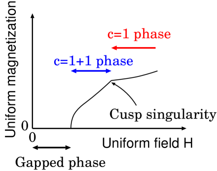
Figure 11: Expected magnetization curves in frustrated integer-spin tubes.

Moreover, the GS phase diagram for the frustrated tubes is drawn as in Fig. 12.

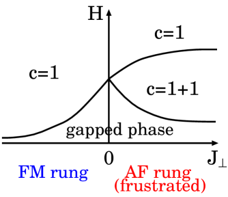
Figure 12: Expected GS phase diagram of odd-leg integer-spin tubes around $(J_{\perp},H)=(0,0)$.

(Applying the same argument to nonfrustrated systems, it is found that the $c=1$ state lasts out even when the condensate of the second lowest magnon occurs.) Besides the above scenario of the magnetization cusp, other cusp singularities have already been found in theoretical studies of 1D quantum systems. Fra-Kre ; Kawa1 ; Kawa2 ; Oku1 ; Oku2 ; Yamamoto It is known that around such cusp points, the left or right derivatives of the magnetization (i.e., susceptibilities) always diverge. However, such a singular phenomena is expected not to occur in our cusp mechanism. Thus, we may insist that the cusp in the frustrated tubes is a new type.

Finally, we remark the validity and the stability of the bosonization arguments in Secs. III.2.2 and III.2.3. The proposal (39) is a strange form: other symmetry operations correspond to a transformation for the phase fields own, but Eq. (39) is the transformation for the vertex operators. In fact, as stated already, Eq. (39) is incompatible with the final term in Eq. (37c). There might be a more natural transformation than Eq. (39). As far as we know, it has never been elucidated whether the GL theory is efficient or not even when multimagnon bands are condensed. Furthermore, the coupling constants of the phase-fields interactions [for example, Eqs. (III.2.3), (III.2.3), and other irrelevant interactions with phase fields] might be as large as the order of $J$. In such a case, the perturbative treatment of them and the biquadratic term $u|\vec{m}|^{4}$ would be dangerous. Thus, there is still a little possibility that the interactions break down the $c=1+1$ state. On the other hand, we essentially use only four symmetries of the spin tubes in order to lead to the $c=1+1$ state. Thus, if our strategy based on the bosonization and the GL theory is admitted, the $c=1+1$ phase must be stabilized against several small perturbations preserving those symmetries (e.g., $XXZ$-type anisotropy, single-ion anisotropy $D\sum_{l,j}(S_{l,j}^{z})^{2}$, next-nearest-neighbor coupling, etc.).

III.3 $[0,\pi]$-field case

This subsection discusses ladders and tubes with the $[0,\pi]$-field term (2b). Odd-leg tubes, which include frustrated tubes, are not admitted in this case.

Imitating the argument in Sec. III.2.1, we can also express the action with the quadratic form of bosons $\tilde{n}_{l}^{\alpha}$, in which ${\bm{E}}_{\omega_{n}}$ is replaced with ${\bm{F}}_{\omega_{n}}=\frac{H\omega_{n}}{gc}{\rm diag}(-1,1,\dots,(-1)^{N})$. In the action, the $2N\times 2N$ matrix held between $\tilde{\cal N}_{\perp}^{\dagger}$ and $\tilde{\cal N}_{\perp}$ are not normal due to ${\bm{F}}_{\omega_{n}}$. Its diagonalization hence generates a nontrivial Jacobian differently from the $[0,0]$-field case. To avoid this difficulty, we turn to the real-time formalism, even though it restricts our consideration to the zero-temperature case. The partition function $Z=\int{\cal D}\vec{n}_{l}{\cal D}\lambda e^{-S_{\rm E}^{[0,\pi]}}$ is associated with the real-time vacuum-vacuum amplitude $Z_{\rm v}=\int{\cal D}\vec{n}_{l}{\cal D}\lambda e^{iS_{\rm R}^{[0,\pi]}}$ via $S_{\rm R}^{[0,\pi]}[t]=iS_{\rm E}^{[0,\pi]}[\tau=it]$. In the Fourier space (note that the frequency $\omega$ is a real number, and not the Matsubara one $\omega_{n}$), the real-time action $S_{\rm R}^{[0,\pi]}$ can be represented as

$$S_{\rm R}^{[0,\pi]}[\{\vec{n}_{l}\},\lambda_{\rm sp}] = \sum_{\bar{\bf k}}\Big{[}\tilde{\cal N}_{\perp}^{R\,{\dagger}}\tilde{\bm{A}}_{\perp}^{R}\tilde{\cal N}_{\perp}^{R}$$ (46)

$$+\tilde{\cal N}_{z}^{R\,{\dagger}}\tilde{\bm{A}}_{z}^{R}\tilde{\cal N}_{z}^{R}\Big{]}-N{\cal T}L\lambda_{\rm sp},$$

where $\bar{\bf k}\equiv(\omega,k)$, $\tilde{\cal N}_{\alpha}^{R}=(n_{1}^{\alpha}(\bar{\bf k}),\dots,n_{N}^{\alpha}(\bar{\bf k}))$, $\tilde{\cal N}_{\perp}^{R}=({}^{T}\tilde{\cal N}_{x}^{R},{}^{T}\tilde{\cal N}_{y}^{R})$, $\cal T$ is the time distance from the initial vacuum to the final one, and we performed a unitary transformation $n_{l}^{y}\to(-1)^{l}n_{l}^{y}$ for convenience. Two matrices $\tilde{\bm{A}}_{\perp}^{R}$ and $\tilde{\bm{A}}_{z}^{R}$ are defined as

$$\tilde{\bm{A}}_{\perp}^{R}(\bar{\bf k}) = \left(\begin{array}[]{ccc}{\bm{A}}_{\bar{\bf k}}&{\bm{E}}_{\omega}\\ -{\bm{E}}_{\omega}&{\bm{B}}_{\bar{\bf k}}\end{array}\right),$$ (47c)

$$\tilde{\bm{A}}_{z}^{R}(\bar{\bf k}) = {\bm{A}}_{\bar{\bf k}}-\frac{H^{2}}{2gc}\hat{\bm{1}},$$ (47d)

$${\bm{E}}_{\omega} = -i\frac{H\omega}{gc}\hat{\bm{1}},$$ (47e)

where ${\bm{A}}_{\bar{\bf k}}$ [${\bm{B}}_{\bar{\bf k}}$] is the same form as ${\bm{A}}_{\bf k}$, in which $\tilde{a}_{1}\to(\omega^{2}-c^{2}k^{2}+2gc\lambda_{\rm sp})/(2gc)$ and $\tilde{a}_{0,2}\to-\tilde{a}_{0,2}$ [$\tilde{a}_{0,2}\to\tilde{a}_{0,2}$]. Since $\tilde{\bm{A}}_{\perp}^{R}$ and $\tilde{\bm{A}}_{z}^{R}$ are Hermite and can be diagonalized by a unitary matrix, we can apply the SPA prescription as in the preceding subsections. Eigenvalues of $\tilde{\bm{A}}_{\perp}^{R}$ and $\tilde{\bm{A}}_{z}^{R}$ are, respectively, $\bar{A}_{r}^{\pm}=(\omega^{2}-\bar{\epsilon}(k)^{2})/(2gc)\pm f_{r}(\bar{\bf k})$ and $\bar{A}_{r}^{z}=(\omega^{2}-\bar{\epsilon}_{r}(k)^{2}-H^{2})/(2gc)$, where we defined

$$\bar{\epsilon}(k)=c\sqrt{k^{2}+\bar{\xi}^{-2}},\,\,\,\,\,\bar{\xi}^{-2}\equiv-2g\lambda_{\rm sp}/c,$$

$$\bar{\epsilon}_{r}(k)=c\sqrt{k^{2}+\bar{\xi}_{r}^{-2}},\,\,\,\,\,\bar{\xi}_{r}^{-2}\equiv\bar{\xi}^{-2}+\frac{2J_{\perp}}{Ja^{2}}\cos k_{r},$$

$$f_{r}(\bar{\bf k})=\sqrt{\left(\frac{cJ_{\perp}}{gJa^{2}}\right)^{2}\cos^{2}k_{r}+\left(\frac{H\omega}{gc}\right)^{2}}.$$

Employing these eigenvalues, one can trace out $\vec{n}_{l}$ in $Z_{\rm v}$, and then obtain the effective action $S_{\rm R}^{[0,\pi]}[\lambda_{\rm sp}]$. The SPE $\partial S_{\rm R}^{[0,\pi]}[\lambda_{\rm sp}]/\partial\lambda_{\rm sp}=0$ can be calculated as

$$\frac{gc}{2\pi}\sum_{r}\int_{0}^{\Lambda}dk\Bigg{[}\sum_{z=0,+,-}\frac{1}{\bar{\epsilon}_{r}^{z}(k)}\,\,\,+\frac{2H^{2}}{h_{r}(k)}\left(\frac{1}{\bar{\epsilon}_{r}^{+}(k)}-\frac{1}{\bar{\epsilon}_{r}^{-}(k)}\right)\Bigg{]} = N,$$ (49)

where

$$\bar{\epsilon}_{r}^{0}(k)=\sqrt{\bar{\epsilon}_{r}(k)^{2}+H^{2}},\,\,\,\,\,\,\,\,\,\,\,\,\,\,\,\bar{\epsilon}_{r}^{\pm}(k)=\sqrt{\bar{\epsilon}(k)^{2}+2H^{2}\pm h_{r}(k)},$$ (50a)

$$h_{r}(k)=\sqrt{4H^{4}+4H^{2}\bar{\epsilon}(k)^{2}+c^{4}\left(\frac{2J_{\perp}}{Ja^{2}}\cos k_{r}\right)^{2}}.$$ (50b)

Here, we used the so-called $i\varepsilon$-prescription Wein in the derivation of the SPE (49). The SPE indicates that $\lambda_{\rm sp}$ is real (not imaginary) and negative in contrast to the imaginary-time schemes. It is verified that as $H\to 0$ [$J_{\perp}\to 0$], Eq. (49) is reduced to the SPE (22) [(14)] of the zero-temperature case, where $(\bar{\xi},\lambda_{\rm sp})$ corresponds to $(\xi,i\lambda_{\rm sp})$.

One can regard $\bar{\epsilon}_{r}^{0,\pm}(k)$ as the magnon band dispersions. At $H=0$, $\bar{\epsilon}_{r}^{0}(k)$, $\bar{\epsilon}_{r}^{+}(k)$, and $\bar{\epsilon}_{r}^{-}(k)$ coincide with $\epsilon_{r}(k)$ in Eq. (20), $\epsilon_{|r|}(k)$ and $\epsilon_{N+1-|r|}(k)$ [$\epsilon_{[\frac{N}{2}]+1-|r|}(k)$], respectively, for ladders [tubes: $N\geq 3$]. Although it is hard to solve the transcendental equation (49) for $\lambda_{\rm sp}$, we can extract some features of the band splitting induced by the $[0,\pi]$ field, from Eqs. (49) and (50). The inequalities $\bar{\epsilon}_{r}^{+}(k)>\bar{\epsilon}_{r}^{-}(k)$ and $h_{r}(k)>2H^{2}\geq 0$ show that the final term in the left-hand side of Eq. (49) is negative or zero. Therefore, $\bar{\xi}^{-2}$ decreases and the bands $\bar{\epsilon}_{r}^{-}(k)$ fall down as $H$ is applied. The form of the dispersion (50a) indicates that as $H$ is applied, the triply degenerate bands $\epsilon_{r}(k)$ with $\cos k_{r}>0$ ($<0$) are split into doubly degenerate upper (lower) bands and a nondegenerate lower (upper) one. The former two are the transverse modes, and the latter is the longitudinal one. The bands with $k_{r}=\pm\frac{\pi}{2}$, which are present only in odd-leg ladders and $(4\times Q)$-leg tubes [$Q\in\mathbb{Z}$], are divided into three bands. From these considerations, we can illustrate the band splitting as in Fig. 13. [Remember that tubes have a sixfold degeneracy in the no-field case (Fig. 4).] The figure tells us three remarkable aspects. (i) Any band $\bar{\epsilon}_{r}^{0,+,-}$ split by the $[0,\pi]$ field tends not to approach the other neighboring bands (to avoid the band crossings). This contrasts with the Zeeman splitting in the uniform ($[0,0]$)-field case, where the crossings among magnon bands with different indices $k_{r}$ occur. (ii) The lowest bands are doubly degenerate in all systems. It might imply that a sufficiently strong $[0,\pi]$ field always engenders a $c=1+1$ phase. (iii) The FM-rung coupling competes with the $[0,\pi]$ field. However, the figure suggests that any qualitative differences between the competitive and noncompetitive cases do not emerge at least in the weak rung-coupling regime.

We believe that the band structure in Fig. 13 is qualitatively valid. However, its details would strongly depend upon the SPA strategy. Particularly, we mind that the symmetry corresponding to the remaining double degeneracy of transverse modes cannot be found. Therefore, the degeneracy and the prediction (ii) would be ruined in more quantitative approaches.

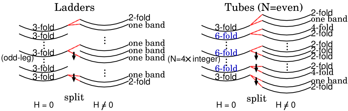
Figure 13: Predicted band splitting in the $[0,\pi]$-field case.

III.4 $[\pi,0]$- and $[\pi,\pi]$-field cases

This subsection addresses the $[\pi,0]$- and $[\pi,\pi]$-field cases, in which the external field is alternated along the chain. Utilizing Eqs. (87) and (18), we can describe their low-energy action as follows:

$$S_{\rm E}[\{\vec{n}_{l}\},\lambda] = \int d{\bf x}\Big{[}{}^{T}{\cal N}_{\alpha}{\bm{A}}{\cal N}_{\alpha}-S\sum_{l}\vec{K}_{l}\cdot\vec{n}_{l}$$ (51)

$$+iN\lambda({\bf x})\Big{]},$$

where $\vec{K}_{l}=\vec{H}/a$ ($\vec{K}_{l}=(-1)^{l+1}\vec{H}/a$) for the $[\pi,0]$-field ($[\pi,\pi]$-field) case [$\vec{H}=(0,0,H)$]. Notice that odd-leg tubes are not permitted for the $[\pi,\pi]$-field case. From Eq. (51), it is found that a unitary transformation $\vec{n}_{l={\rm even}}\to-\vec{n}_{l={\rm even}}$ exchanges the action of the AF (FM)-rung system with the $[\pi,\pi]$ field into that of the FM (AF)-rung one with the $[\pi,0]$ field. Therefore, it is enough to investigate only either $[\pi,0]$-field case or the $[\pi,\pi]$-field case. We analyze the former case below.

After diagonalizing the quadratic part of $\vec{n}_{l}$ in Eq. (51), the action are arranged as

$$S_{\rm E}^{[\pi,0]}[\{\vec{n}_{l}\},\lambda] = \int d{\bf x}\Big{[}\sum_{r}\Big{\{}\vec{m}_{r}({\bf x})A_{r}({\bf x})\vec{m}_{r}({\bf x})$$ (52)

$$-S\vec{J}_{r}\cdot\vec{m}_{r}\Big{\}}+iN\lambda({\bf x})\Big{]},$$

where

$$A_{r}({\bf x})=-\frac{1}{gc}\Big{[}\partial_{\tau}^{2}+c^{2}\partial_{x}^{2}+\xi_{r}({\bf x})^{-2}\Big{]},\hskip 28.45274pt\xi_{r}({\bf x})^{-2}=\frac{-2ig\lambda({\bf x})}{c}+\frac{2J_{\perp}}{Ja^{2}}\cos k_{r},\hskip 28.45274pt$$ (53a)

$$\vec{J}_{r}=\left\{\begin{array}[]{cc}\delta_{r,{\rm odd}}\sqrt{\frac{2}{N+1}}\left[\tan\left(\frac{r\pi}{2(N+1)}\right)\right]^{-1}\frac{\vec{H}}{a}&({\rm ladders})\\ \delta_{r,0}\sqrt{N}\frac{\vec{H}}{a}&({\rm tubes}:\,\,N\geq 3),\end{array}\right.\,\,\,\,$$ (53d)

and the field $\vec{m}_{r}({\bf x})=U_{rl}\vec{n}_{l}$ [see Eq. (29a)]. The action (52) can be considered as a generalization of that of the single chain with a staggered field (87). Thus, we can apply the Green’s function method in Appendix B to the present $[\pi,0]$-field case. (We would like the reader to refer Appendix B or Ref. Erco, before proceeding below.)

Following Appendix B, let us define Green’s functions:

$$A_{r}({\bf x})G_{r}^{0}({\bf x}-{\bf x^{\prime}}) = \delta^{2}({\bf x}-{\bf x^{\prime}}),$$ (54a)

$$G_{r}^{T}({\bf x}-{\bf x^{\prime}}) = \langle{\cal T}_{\tau}m_{r}^{x(y)}({\bf x})m_{r}^{x(y)}({\bf x^{\prime}})\rangle_{c},$$ (54b)

$$G_{r}^{L}({\bf x}-{\bf x^{\prime}}) = \langle{\cal T}_{\tau}m_{r}^{z}({\bf x})m_{r}^{z}({\bf x^{\prime}})\rangle_{c},$$ (54c)

where the subscript _c means “connected,” ${\cal T}_{\tau}$ denotes imaginary-time ordered product [see Eq. (B)], and $\delta^{2}({\bf x}-{\bf x^{\prime}})=\delta(x-x^{\prime})\delta(\tau-\tau^{\prime})$. In anticipation of removing the space-time dependence of $\xi_{r}$ via the SPA process, we already assumed that the above Green’s functions depend only on the distance between ${\bf x}$ and ${\bf x^{\prime}}$. The magnon dispersions of transverse and longitudinal modes can be determined from $G_{r}^{T}({\bf x}-{\bf x^{\prime}})$ and $G_{r}^{L}({\bf x}-{\bf x^{\prime}})$, respectively. As in Eq. (96), the Fourier transformation of $G_{r}^{0}$ is estimated as

$$\tilde{G}_{r}^{0}({\bf k}) = \frac{gc}{\omega_{n}^{2}+c^{2}k^{2}+c^{2}\xi_{r}^{-2}},$$ (55)

where $\xi_{r}^{-2}=-\frac{2ig\lambda{\rm sp}}{c}+\frac{2J_{\perp}}{Ja^{2}}\cos k_{r}$ and $\lambda_{\rm sp}$ is the saddle-point value of $\lambda({\bf x})$. Using $\tilde{G}_{r}^{0}$ and referring the way deriving Eqs. (B) and (97), we obtain the following SPE determining $\lambda_{\rm sp}$ and $\xi_{r}$,

$$\frac{3gc}{2\pi}\sum_{r}\int\frac{dk}{\epsilon_{r}(k)}\coth\left(\frac{\beta}{2}\epsilon_{r}(k)\right)$$

$$=N-S^{2}\sum_{r}{\vec{J}_{r}}^{2}\left(\frac{g}{c}\right)^{2}\xi_{r}^{4},$$ (56)

where the final term in the right-hand side represents the $[\pi,0]$-field effect. As $J_{\perp}\to 0$, Eq. (III.4) returns to Eq. (97). Applying Eqs. (91) and (98), we further evaluate the staggered magnetization as

$$\vec{M}_{l} \equiv S\langle\vec{n}_{l}\rangle=S\sum_{r}U_{rl}\langle\vec{m}_{r}\rangle=\left\{\begin{array}[]{cc}\frac{2}{N+1}\sum_{r=1}^{N}\delta_{r,{\rm odd}}\sin\left(\frac{rl\pi}{N+1}\right)\left[\tan\left(\frac{r\pi}{2(N+1)}\right)\right]^{-1}\left(\frac{\xi_{r}}{a}\right)^{2}\frac{\vec{H}}{J}&({\rm ladders})\\ \left(\frac{\xi_{0}}{a}\right)^{2}\frac{\vec{H}}{J}&({\rm tubes}:\,N\geq 3)\end{array}\right.,\,\,\,\,\,\,\,$$ (59)

where $\vec{M}_{l}$ is parallel to the field $\vec{H}$ like the single-chain case [see Eq. (98)], namely $\vec{M}_{l}=(0,0,M_{l})$. The staggered magnetizations are independent of the chain index $l$ in the tubes: $M_{l}=M_{s}$. On the other hand, the $l$-dependence of the magnetizations clearly exists in the ladders. We emphasize that these inhomogeneous distribution of the staggered magnetization cannot be predicted by the standard NLSM scheme, which assumes a short-range AF or FM order to arise for the rung direction. From $\sin(\frac{rl\pi}{N+1})=\sin(\frac{r(N+1-l)\pi}{N+1})$, we find that $M_{l}=M_{N+1-l}$ is realized in the ladders. The results $M_{l}=M_{s}$ in tubes and $M_{l}=M_{N+1-l}$ in ladders indicate that the present NLSM plus SPA scheme preserves the translational symmetry along the rung in tubes, and the reflection one about the plane containing the central axis of the ladder, in the $[\pi,0]$-field case [refer to the discussion about the validity of Eqs. (16) and (17) in Sec. III.1].

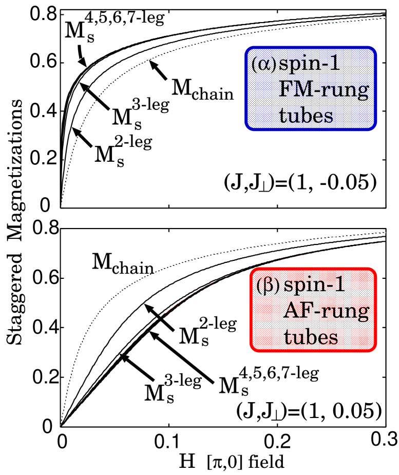
Figure 14: Staggered magnetizations of $N$-leg spin-$1$ FM- or AF-rung tubes with the $[\pi,0]$ field, $M_{s}^{\text{N-leg}}$. The dotted curve $M_{\rm chain}$ stands for the staggered magnetization $m_{s}^{z}$ of the single AF chain with the staggered field (see Fig. 1). The 2-leg tube means the 2-leg ladder. A relation $M_{s}^{\text{p-leg}}(H)<M_{s}^{\text{(p+1)-leg}}(H)$ [$M_{s}^{\text{p-leg}}(H)>M_{s}^{\text{(p+1)-leg}}(H)$] is realized for the FM [AF]-rung case. Magnetizations $M_{s}^{\text{4,5,6,7-leg}}$ almost overlap.

We will investigate the magnetizations $\vec{M}_{l}$ and the magnon modes in detail, below.

III.4.1 Staggered Magnetizations

If $\lambda_{\rm sp}$ is fixed by the SPE, the magnetizations $\vec{M}_{l}$ are also done in Eq. (59). Figures 14-16 display them in zero temperature. The FM rung coupling and the $[\pi,0]$ field are cooperative each other, while the AF rung coupling competes with the field. A consequence is, as shown in Fig. 14, that for FM (AF)-rung tubes, $M_{s}$ are always larger (smaller) than that of the single AF chain with a staggered field. In addition, the growth of $N$ gradually enhances (reduces) the magnetization $M_{s}$ in FM (AF)-rung tubes. The magnetization profile such as the panel ($\alpha$) in Fig. 14 is also expected in nonfrustrated (FM-rung) ladders. Actually, as expected, Fig. 15 indicates that for the small-field regime $H\lesssim 0.05$, $M_{l}$ tend to increase together the growth of $N$. It further explains that the more the $l$th chain approaches the center of the ladder, the larger its magnetization $M_{l}$ becomes. This is understood from the consideration that the chains near the center are more subject to the FM-rung correlation effects than ones near the edge. On the other hand, one can extract following two unexpected features in Fig. 15. (i) The maximum magnetization in $M_{l}$ of the $N$-leg ladder, $M_{\rm max}^{N}$, is slightly larger than that of $(N+1)$-leg ladder for the regime $H\gtrsim 0.05$ and $N\geq 3$. (ii) The edge magnetization $M_{1,N}$ is smaller than that of the single chain in the same regime. Since the $[\pi,0]$ field and FM rung coupling, which is absent in the single chains, must cooperatively enhance the growth of $M_{l}$, these two results are expected to be incorrect. Because in the spin-1 AF chain, the staggered magnetization obtained by the SPA is almost consistent with the DMRG data within $0\leq\frac{H}{J}\leq 0.5$, Erco these unexpected results would mainly originate from the averaging of constraints, Eq. (17). The approximation (17) would prevent $M_{l}$ from increasing in the regime $H\gtrsim 0.05$. The true magnetization curves are expected to have a less $l$-dependence so that the edge magnetization $M_{1,N}$ is always larger than that of the single chain, $M_{\rm chain}$ in Fig. 15. Moreover, $M_{\rm max}^{N+1}>M_{\rm max}^{N(\geq 3)}$ must hold for all region $0\leq H<\infty$ in the FM-rung ladders.

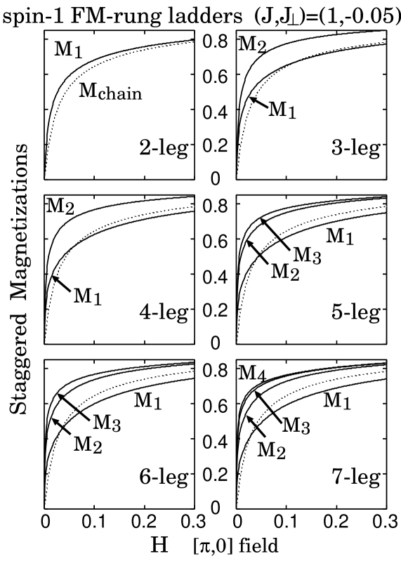
Figure 15: Staggered magnetizations of $N$-leg spin-$1$ FM-rung ladders with the $[\pi,0]$ field and $J_{\perp}/J=-0.05$. For $l<[\frac{N}{2}]$, $M_{l+1}(H)>M_{l}(H)$ is realized. Similarly to Fig. 14, the symbol $M_{\rm chain}$ means $m_{s}^{z}$.

Figure 16 provides the staggered magnetizations in the frustrated AF-rung ladders with the $[\pi,0]$ field. The left panel [a] insists that the staggered magnetizations tend to point to the same direction as the $[\pi,0]$ field, when the AF rung coupling is small enough; $\frac{J_{\perp}}{J}\lesssim 0.03$. The edge magnetization $M_{1,N}$ increases most rapidly in such a weak rung-coupling region since the edge chain receives the competitive AF rung coupling from only one side, unlike other chains. The rapid growth of $M_{1,N}$ and the AF rung coupling would make the growths of $M_{l=\text{even}}$ slower. While, the panel [b] contains the following interesting phenomena: when the $[\pi,0]$ field and the rung coupling are sufficiently small and large, respectively ($\frac{H}{J}\lesssim 0.1$ and $\frac{J_{\perp}}{J}\gtrsim 0.03$) in the odd-leg tubes, the field induces the staggered magnetization pointing to the opposite direction to it in the even-$l$ chains. This result is unique for the ladders, and does not appear in AF-rung tubes (see Fig. 14). Such a magnetization configuration staggered along the rung does not also occur in even-leg ladders, because the configuration cannot be compatible with the edge magnetization turning to the $[\pi,0]$ field. One may call the result in the panel [b] as an even-odd property in the ladders with the $[\pi,0]$ field. Although the panel [b] further implies the simultaneous crossings of $(M_{1},M_{3})$ and $(M_{2},M_{4},\text{zero-magnetization line})$, they might be a coincidence depending on the approximation (17). From the discussion about Fig. 15, Fig. 16 might be also less accurate for the regime $H\gtrsim 0.05$.

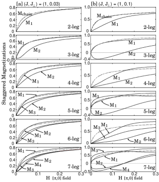
Figure 16: Staggered magnetizations $M_{l}$ of $N$-leg spin-$1$ AF-rung ladders with the $[\pi,0]$ field.

III.4.2 Magnon Dispersions

We next study the magnon dispersions of the $[\pi,0]$-field case. Following the functional derivative technique such as Eq. (B), we can represent $G_{r}^{T(L)}$ as

$$G_{r}^{T(L)}({\bf x}-{\bf x^{\prime}})=S^{2}G_{r}^{0}({\bf x}-{\bf x^{\prime}})+2S^{2}\int d{\bf y}\bigg{[}$$

$$G_{r}^{0}({\bf x}-{\bf y})G_{r}^{0}({\bf y}-{\bf z})J_{r}^{x(z)}({\bf z})\Big{(}i\frac{\delta\lambda({\bf y})}{\delta J_{r}^{x(z)}({\bf x^{\prime}})}\Big{)}\bigg{]}.$$ (60)

In the calculation of $\delta\lambda/\delta J_{r}^{\alpha}$, we suppose that each $J_{r}^{\alpha}$ is an independent external field. The relation $J_{r}^{x,y}=0$ leads to $G_{r}^{T}({\bf x})=S^{2}G_{r}^{0}({\bf x})$. The Fourier transformation of $G_{r}^{T}$ is

$$\tilde{G}_{r}^{T}({\bf k}) = \frac{S^{2}gc}{\omega_{n}^{2}+\epsilon_{r}(k)^{2}}.$$ (61)

Therefore, we can immediately conclude that the dispersion of the $r$-th transverse mode $\epsilon_{r}^{T}(k)$ is given by $\epsilon_{r}(k)$. Similarly to the single-chain case, this mode has the double degeneracy corresponding to the $x$ and $y$ components. Furthermore, like the no-field case, the tubes exhibit the four-fold degeneracy $\epsilon_{r}=\epsilon_{-r}$ except for $r=0$ and $\frac{N}{2}$ modes. The SPE (III.4) tells us that $\xi^{-2}=-\frac{2ig\lambda_{\rm sp}}{c}$ is enhanced by the field $H$ (or $J_{r}^{z}$). The transverse bands $\epsilon_{r}^{T}(k)$ and gaps $\Delta_{r}^{T}\equiv\epsilon_{r}^{T}(0)$ hence rise monotonically with $H$ increasing.

Although the estimation of the longitudinal mode $\epsilon_{r}^{L}(k)$ is rather complicated due to the presence of $J_{r}^{z}$, it is possible through the application of the method of deriving $\epsilon_{L}(k)$ in the single chain with a staggered field. The trivial relation $\frac{\delta}{\delta J_{r}^{z}}(\frac{\delta S_{\rm E}^{[\pi,0]}}{\delta\lambda})=0$ is available as the integral equation determining $\delta\lambda/\delta J_{r}^{z}$ in Eq. (III.4.2). Imitating Eqs. (B)-(B), we can transform it as follows:

$$\int d{\bf y}I({\bf x}-{\bf y})\Big{(}i\frac{\delta\lambda({\bf y})}{\delta J_{r}^{z}({\bf x^{\prime}})}\Big{)} = -2{\cal M}_{r}G_{r}^{0}({\bf x}-{\bf x^{\prime}}),\,\,\,\,\,$$ (62)

where

$${\cal M}_{r} = S\langle m_{r}^{z}\rangle=S^{2}\tilde{G}_{r}^{0}({\bf 0})H/a,$$ (63a)

$$I({\bf x}-{\bf y}) = \sum_{r}\Big{[}6\Gamma_{r}({\bf x}-{\bf y})$$ (63b)

$$+({\cal M}_{r}/S)^{2}G_{r}^{0}({\bf x}-{\bf y})\Big{]},$$

$$\Gamma_{r}({\bf x}-{\bf y}) = G_{r}^{0}({\bf x}-{\bf y})G_{r}^{0}({\bf y}-{\bf x}).$$ (63c)

Equations (III.4.2) and (62) lead to the following expression for the Fourier transformation of $G_{r}^{L}$:

$$\tilde{G}_{r}^{L}({\bf k}) = \tilde{G}_{r}^{T}({\bf k})\frac{\sum_{p}3\tilde{\Gamma}_{p}({\bf k})+\sum_{p\neq r}2\tilde{\cal M}_{p}^{2}\tilde{G}_{p}({\bf k})}{\sum_{p}[3\tilde{\Gamma}_{p}({\bf k})+2\tilde{\cal M}_{p}^{2}\tilde{G}_{p}({\bf k})]},\,\,\,\,\,\,\,\,\,\,\,\,$$ (64)

where $\tilde{\cal M}_{r}={\cal M}_{r}/S=\langle m_{r}^{z}\rangle$. The longitudinal mode $\epsilon_{r}^{L}(k)$ can be fixed by the pole structures of the real-time retarded Green’s function $\tilde{G}_{r}^{L}(\bar{\bf k})\equiv\tilde{G}_{r}^{L}({\bf k})|_{\omega_{n}\to-iz}$, where $\bar{\bf k}=(z,k)$, $z=\omega+i\eta$, and $\eta\to+0$. Here, as in Eq. (101), let us introduce new symbols,

$$G_{r}(z) = \tilde{G}_{r}^{L}(\bar{\bf k})/(S^{2}gc),$$ (65a)

$$\Gamma_{r}(z) = 3\tilde{\Gamma}_{p}(\bar{\bf k})/(2gc),$$ (65b)

$$\Gamma_{\text{tot}}(z) = \sum_{r}\Gamma_{r}(z),$$ (65c)

$${\cal F}^{1(2)}(z) = \mathfrak{Re}(\mathfrak{Im}){\cal F}(z),$$ (65d)

where we omit the subscript $k$, and ${\cal F}(z)$ is an arbitrary function of $\bar{\bf k}$. In terms of these symbols, we obtain the simplified expression of the real-time Green’s function,

$$G_{r}(z) = \frac{\Gamma_{\text{tot}}(z)+\sum_{p\neq r}\frac{\tilde{\cal M}_{p}^{2}}{\epsilon_{p}(k)^{2}-z^{2}}}{(\epsilon_{r}(k)^{2}-z^{2})\big{[}\Gamma_{\text{tot}}(z)+\sum_{p}\frac{\tilde{\cal M}_{p}^{2}}{\epsilon_{p}(k)^{2}-z^{2}}\big{]}}.\,\,\,\,\,\,\,\,\,\,$$ (66)

Analyzing Eq. (66), one can find the longitudinal magnon dispersions.

[Tubes] The calculation of $G_{r}(z)$ in the tubes is easier than that in the ladders, because the tubes take $J_{r}^{z}\propto\delta_{r,0}$ and $\tilde{\cal M}_{r}\propto\delta_{r,0}$. These properties bring

$$G_{r\neq 0}(z) = \frac{1}{\epsilon_{r}(k)^{2}-z^{2}}\propto\tilde{G}_{r}^{T}(\bar{\bf k}).$$ (67)

The longitudinal dispersion $\epsilon_{r}^{L}(k)$, thus, is equivalent to the transverse one $\epsilon_{r}^{T}(k)$ for $r\neq 0$. Namely, in the tubes with the $[\pi,0]$ field, the $r$th magnon mode is triply degenerate like the zero-field case (Fig. 4), except for the $0$th mode. Of course, there exists the additional degeneracy $\epsilon_{r}=\epsilon_{-r}$. On the other hand, the $0$th mode Green’s function is written as

$$G_{0}(z) = \frac{\Gamma_{\text{tot}}(z)}{(\epsilon_{0}(k)^{2}-z^{2})\Gamma_{\text{tot}}(z)+\tilde{\cal M}_{0}^{2}}.$$ (68)

The form of $G_{0}(z)$ is quite similar to that of $G(z)$ in Eq. (103). Moreover, at $T=0$, $\Gamma_{r}^{1,2}(z)$ have the same form as $\Gamma^{1,2}$ fixed by Eq. (102). Therefore, following the calculation from Eq. (104) to Eq. (108), we can achieve, at $T=0$,

$$\epsilon_{0}^{L}(k)^{2} = \epsilon_{0}^{T}(k)^{2}+\tilde{\cal M}_{0}^{2}/\Gamma_{\rm{tot}}^{1}(\epsilon_{0}^{L}(k),k),$$ (69)

where we restore the subscript $k$ in $\Gamma_{\rm{tot}}^{1}$. Note that in the derivation of Eq. (69), we assume $\epsilon_{0}^{L}(k)<2\epsilon_{\text{min}}(k/2)$, where $\epsilon_{\text{min}}(k)$ is defined as the minimum of all the transverse dispersions $\epsilon_{r}(k)$ (see Fig. 4). Because the inequality $\Gamma_{\rm{tot}}^{1}(\epsilon_{0}^{L}(k),k)>0$ is realized under $\epsilon_{0}^{L}(k)<2\epsilon_{\text{min}}(k/2)$, Eq. (69) explains that the $0$th longitudinal band $\epsilon_{0}^{L}(k)$ is always larger than the transverse one $\epsilon_{0}^{T}(k)$. Employing the explicit form of $\Gamma_{r}^{1}(\epsilon_{0}^{L}(0),0)$ [see Eq. (107)], we can calculate the longitudinal gap $\Delta_{0}^{L}\equiv\epsilon_{0}^{L}(0)$ as follows:

$${\Delta_{0}^{L}}^{2} = {\Delta_{0}^{T}}^{2}+\frac{2\tilde{\cal M}_{0}^{2}}{3g}\Big{[}\sum_{r}{\Delta_{r}^{T}}^{-2}K(\Delta_{0}^{L}/\Delta_{r}^{T})\Big{]}^{-1},\,\,\,\,\,$$ (70)

where

$$K(x) = \frac{1}{2\pi x\sqrt{1-x^{2}/4}}\arctan\left(\frac{x}{2\sqrt{1-x^{2}/4}}\right),\,\,\,\,\,\,$$ (71)

and we, of course, assumed that the minimum point of the band $\epsilon_{0}^{L}(k)$ is located at $k=0$. The SPE (III.4) and Eqs. (67)-(70) enable us to know all the magnon band structures in the tubes ($N\geq 3$) with the $[\pi,0]$ field at $T=0$.

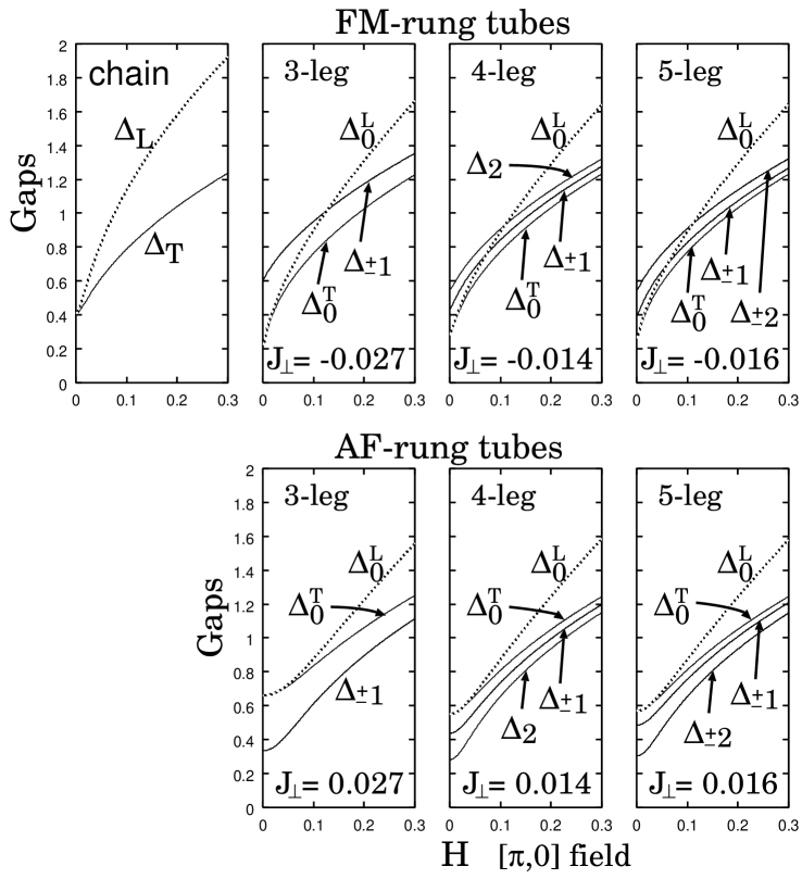
Figure 17: Transverse and longitudinal gaps of $N$-leg spin-$1$ tubes ($N\geq 3$) with the $[\pi,0]$ field and $J=1$. As a comparison, we also draw the gaps of the spin-$1$ chain with staggered field (see Fig. 2) in the left upper panel.

Figure 17 shows the gaps $\Delta_{r}^{T,L}$ at $T=0$. In this figure, we see that $\Delta_{r}^{T}=\Delta_{r}^{L}\equiv\Delta_{r}$ holds for $r\neq 0$. Since the strong rung coupling destroys the condition $\epsilon_{0}^{L}(k)<2\epsilon_{\text{min}}(k/2)$, our scope in Fig. 17 is restricted to the extremely weak rung-coupling regime. We, however, believe that the gap behavior in Fig. 17 is robust even with a moderately strong rung coupling. The lowest (highest) band $\epsilon_{0}$ is split by the field in the FM (AF)-rung tubes. Thus, there are the magnon-band crossings only in the FM-rung tubes. The manner of the lowest-band splitting goes for that of the single chain with the staggered field (see the upper panels in Fig. 17, and Fig. 2). It implies that an $N$-leg spin-$S$ FM-rung tube has the same low-energy properties as the spin-$(N\times S)$ single chain even for the weak rung-coupling regime. The growths of gaps in the AF-rung case are slightly slower than those in the FM-rung case. It must reflect the frustration between the rung coupling and the field. As already predicted, one can verify from Fig. 17 that all the gaps monotonically grow up with $H$ increasing. We, thus, conclude that in tubes the $[\pi,0]$ field induces no critical phenomena at least in the weak rung-coupling regime, irrespective of the presence of the frustration. Although the SPA predicts that only the degeneracy of the bands $\epsilon_{0}$ is lifted by the field, actually the other bands are also expected to more or less split (because any mechanisms preserving the triple degeneracy of magnon bands are not found in the $[\pi,0]$-field case).

[2-leg ladder] Let us next investigate the longitudinal magnons for the ladders. For the 2-leg case, the estimation of $G_{r}$ is as simple as that in the tubes because of $J_{2}^{z}={\cal M}_{2}=0$, which leads to $G_{2}(z)\propto G_{2}^{T}(\bar{\bf k})$. Therefore, the dispersion of the longitudinal mode $\epsilon_{2}^{L}(k)$ is identical with $\epsilon_{2}^{T}(k)$. On the other hand, $G_{1}$ is written as

$$G_{1}(z) = \frac{\Gamma_{\text{tot}}(z)}{(\epsilon_{1}(k)^{2}-z^{2})\Gamma_{\text{tot}}(z)+\tilde{\cal M}_{1}^{2}}.$$ (72)

Because the form of $G_{1}$ is same as Eq. (68), the process from Eq. (68) to Eq. (71) can be directly applied as a way determining the longitudinal dispersion $\epsilon_{1}^{L}(k)$. As a result, at $T=0$, we obtain two equations,

$$\epsilon_{1}^{L}(k)^{2} = \epsilon_{1}^{T}(k)^{2}+\tilde{\cal M}_{1}^{2}/\Gamma_{\rm{tot}}^{1}(\epsilon_{1}^{L}(k),k),$$ (73a)

$${\Delta_{1}^{L}}^{2} = {\Delta_{1}^{T}}^{2}+\frac{2\tilde{\cal M}_{1}^{2}}{3g}\Big{[}\sum_{r=1}^{2}{\Delta_{r}^{T}}^{-2}K(\Delta_{1}^{L}/\Delta_{r}^{T})\Big{]}^{-1},\,\,\,\,\,\,\,\,\,\,\,\,\,\,$$ (73b)

under the condition $\epsilon_{1}^{L}(k)<2\epsilon_{\rm{min}}(k/2)$. Equation (73a) indicates $[2\epsilon_{\rm{min}}(k/2)>]$ $\epsilon_{1}^{L}(k)>\epsilon_{1}^{T}(k)$.

[3-leg ladder] Like $G_{2}$ in the 2-leg ladder, ${\cal M}_{2}=0$ leads to $\epsilon_{2}^{L}(k)=\epsilon_{2}^{T}(k)$ in the 3-leg ladder. On the other hand, $G_{1,3}$ are more complicated than the Green’s functions in the 2-leg case. After a simple calculation, they are represented as

$$G_{1,3}(z) = \frac{{\cal C}_{1,3}(\omega)+i{\cal D}_{1,3}(\omega)}{{\cal A}(\omega)+i{\cal B}(\omega)},$$ (74)

where

$${\cal A} = E_{1}E_{3}\Gamma_{\rm{tot}}^{1}(z)+\tilde{\cal M}_{1}^{2}E_{3}+\tilde{\cal M}_{3}^{2}E_{1}$$ (75a)

$$+2\eta\omega(E_{1}+E_{3})\Gamma_{\rm{tot}}^{2}(z)-4\eta^{2}\omega^{2}\Gamma_{\rm{tot}}^{1}(z),\,\,\,\,\,\,$$

$${\cal B} = E_{1}E_{3}\Gamma_{\rm{tot}}^{2}(z)-2\eta\omega(E_{1}+E_{3})\Gamma_{\rm{tot}}^{1}(z)$$ (75b)

$$-2\eta\omega(\tilde{\cal M}_{1}^{2}+\tilde{\cal M}_{3}^{2})-4\eta^{2}\omega^{2}\Gamma_{\rm{tot}}^{2}(z),$$

$${\cal C}_{1(3)} = E_{3(1)}\Gamma_{\rm{tot}}^{1}(z)+2\eta\omega\Gamma_{\rm{tot}}^{2}(z)+\tilde{\cal M}_{3(1)}^{2},$$ (75c)

$${\cal D}_{1(3)} = E_{3(1)}\Gamma_{\rm{tot}}^{2}(z)-2\eta\omega\Gamma_{\rm{tot}}^{1}(z),$$ (75d)

$$E_{r} = \epsilon_{r}(k)^{2}-\omega^{2}+\eta^{2}.$$ (75e)

Under the condition $|\omega|<2\epsilon_{\rm{min}}(k/2)$ and $T=0$, in which $\Gamma_{\rm{tot}}^{1}>0$ and $\Gamma_{\rm{tot}}^{2}=0$, $G_{1,3}$ are fairly simplified. In that case, the explicit forms of their imaginary part are

$$G_{1,3}^{2}(z)=\frac{2\eta\omega\Big{[}(E_{3}\Gamma_{\rm{tot}}^{1}+\tilde{\cal M}_{3})^{2}+\tilde{\cal M}_{1}^{2}\tilde{\cal M}_{3}^{2}+{\cal E}_{1,3}\Big{]}}{\Big{[}E_{1}E_{3}\Gamma_{\rm{tot}}^{1}+\tilde{\cal M}_{1}^{2}E_{3}+\tilde{\cal M}_{3}^{2}E_{1}-4\eta^{2}\omega^{2}\Gamma_{\rm{tot}}^{1}\Big{]}^{2}+4\eta^{2}\omega^{2}\Big{[}(E_{1}+E_{3})\Gamma_{\rm{tot}}^{1}+\tilde{\cal M}_{1}^{2}+\tilde{\cal M}_{3}^{2}\Big{]}^{2}},$$ (76)

where ${\cal E}_{1}=4\eta^{2}\omega^{2}(\Gamma_{\rm{tot}}^{1})^{2}$ and ${\cal E}_{3}=4\eta^{2}\omega^{2}$. At the limit $\eta\to+0$ [see Eq. (105)], both $G_{1}^{2}$ and $G_{3}^{2}$ take the same pole structure as follows:

$$\lim_{\eta\to+0}G_{1,3}^{2}\propto\delta(g(\omega)), g(\omega)=\frac{E_{1}E_{3}\Gamma_{\rm{tot}}^{1}(\omega)+\tilde{\cal M}_{1}^{2}E_{3}+\tilde{\cal M}_{3}^{2}E_{1}}{(E_{1}+E_{3})\Gamma_{\rm{tot}}^{1}(\omega)+\tilde{\cal M}_{1}^{2}+\tilde{\cal M}_{3}^{2}}.$$ (77)

From the solution of $g(\omega)=0$, we obtain the following two longitudinal bands $\epsilon_{\pm}^{L}(k)$:

$$\epsilon_{\pm}^{L}(k)^{2}=\frac{1}{2}\Big{[}\epsilon_{1}(k)^{2}+\epsilon_{3}(k)^{2}\Big{]}+\frac{1}{2\Gamma_{\rm{tot}}^{1}}(\tilde{\cal M}_{1}^{2}+\tilde{\cal M}_{3}^{2})\hskip 236.15796pt$$

$$\pm\frac{1}{2\Gamma_{\rm{tot}}^{1}}\sqrt{\Big{[}(\epsilon_{1}(k)^{2}+\epsilon_{3}(k)^{2})\Gamma_{\rm{tot}}^{1}+\tilde{\cal M}_{1}^{2}+\tilde{\cal M}_{3}^{2}\Big{]}^{2}-4\Gamma_{\rm{tot}}^{1}\Big{[}\epsilon_{1}(k)^{2}\epsilon_{3}(k)^{2}\Gamma_{\rm{tot}}^{1}+\tilde{\cal M}_{1}^{2}\epsilon_{3}(k)^{2}+\tilde{\cal M}_{3}^{2}\epsilon_{1}(k)^{2}\Big{]}},$$ (78)

where $\Gamma_{\rm{tot}}^{1}$ means $\Gamma_{\rm{tot}}^{1}(\epsilon_{\pm}^{L}(k),k)$. From this result, it is clear that at least within the SPA scheme, the $[\pi,0]$ field engenders the hybridization between two magnon bands $\epsilon_{1}$ and $\epsilon_{3}$ in the 3-leg ladders. Provided that the minimum of $\epsilon_{\pm}^{L}(k)$ is in $k=0$, the gap $\Delta_{\pm}^{L}=\epsilon_{\pm}^{L}(0)$ can be determined by the replacement $(\epsilon_{\pm}^{L},\epsilon_{1},\epsilon_{3})\to(\Delta_{\pm}^{L},\Delta_{1},\Delta_{3})$ in Eq. (III.4.2). In the zero-field limit $H\to 0$, where $\tilde{\cal M}_{1,3}\to 0$, Eq. (III.4.2) reduces to

$$\epsilon_{\pm}^{L}(k)^{2} \approx \frac{1}{2}\Big{[}\epsilon_{1}(k)^{2}+\epsilon_{3}(k)^{2}\pm\big{|}\epsilon_{1}(k)^{2}-\epsilon_{3}(k)^{2}\big{|}\Big{]}.\,\,\,\,$$ (79)

This result and the inequality $\epsilon_{1}(k)<\epsilon_{3}(k)$ [$\epsilon_{1}(k)>\epsilon_{3}(k)$] in the FM [AF]-rung ladder reveal that $\epsilon_{+}^{L}$ and $\epsilon_{-}^{L}$ are, respectively, split from $\epsilon_{3}$ and $\epsilon_{1}$ ($\epsilon_{1}$ and $\epsilon_{3}$) in the FM (AF)-rung ladder. Therefore, $\epsilon_{+}^{L}$ and $\epsilon_{-}^{L}$ should be rewritten as $\epsilon_{3}^{L}$ and $\epsilon_{1}^{L}$ ($\epsilon_{1}^{L}$ and $\epsilon_{3}^{L}$) for the FM (AF)-rung ladder. The gaps $\Delta_{\pm}^{L}$ also can be redefined.

[4-leg and higher-leg ladders] The logic calculating the longitudinal dispersions in the 2- and 3-leg ladders is successful even for the 4-leg ladders. We mention only the results of them. The identities ${\cal M}_{2,4}=0$ leads to $\epsilon_{2,4}^{L}(k)=\epsilon_{2,4}^{T}(k)$. While, $G_{1,3}(z)$ take the same form as Eq. (76) under the condition $|\omega|<2\epsilon_{\rm{min}}(k/2)$, except that $\Gamma_{\rm{tot}}^{1}=\sum_{r=1}^{3}\Gamma_{r}^{1}$ and $k_{r}=\frac{r\pi}{4}$ are replaced with $\sum_{r=1}^{4}\Gamma_{r}^{1}$ and $k_{r}=\frac{r\pi}{5}$, respectively. Therefore, $\epsilon_{1,3}^{L}(k)$ can be fixed like Eq. (III.4.2). As easily expected, the evaluations of the magnon dispersions in the higher-leg ladders demand the more complicated analyses. Here we do not perform them. In principle, one can study all the longitudinal bands using Eq. (66).

We show the gaps of 2, 3, and 4-leg ladders in Fig. 18. The gap behavior is much similar to that of the tubes in Fig. 17: the highest (lowest) band is largely split into the doubly degenerate transverse bands and the single longitudinal band in the FM (AF)-rung ladders. The splitting of $\epsilon_{3}(k)$ is considerably small. Namely, $\Delta_{3}^{L}$ and $\Delta_{3}^{T}$ almost overlap. Observing carefully the numerical data of 3-leg and 4-leg FM-rung ladders, we see that $\Delta_{3}^{L}$ ($\Delta_{3}^{T}$) is a little larger than $\Delta_{3}^{T}$ ($\Delta_{3}^{L}$) for the case $\Delta_{1}^{L}<\Delta_{3}^{T}$ ($\Delta_{1}^{L}>\Delta_{3}^{T}$). Even though the band crossings in FM-rung tubes (Fig. 17) are allowed from the translational symmetry along the rung, the ladders do not possess such a symmetry. Therefore, the level crossing in Fig. 18 might, in fact, be an avoided crossing. Moreover, more quantitative analyses would lift the remaining triple degeneracy of the bands $\epsilon_{1,2}$ in Fig. 18.

Summarizing all the discussions about the magnon dispersions, we can conclude that the $[\pi,0]$ field engenders the monotonic raise of all magnon bands, and cannot induce any critical phenomena at least for the weak rung-coupling regime. While, we have already predicted that the other staggered field, the $[0,\pi]$ field, induces the gap reduction (Fig. 13). Therefore, our results in the $[0,\pi]$, $[\pi,0]$, and $[\pi,\pi]$-field cases suggest that the spatial direction with the staggered component of the fields essentially affects the low-energy excitations of the spin ladders and tubes.

Figure 18: Transverse and longitudinal gaps of $N$-leg spin-$1$ ladders with the $[\pi,0]$ field and $J=1$. The gaps $\Delta_{3}^{T}$ and $\Delta_{3}^{L}$ almost overlap.

Finally, we notice again that through the transformation $\vec{n}_{l=\rm{even}}\to-\vec{n}_{l=\rm{even}}$, all the results in Figs. 14-18 can be interpreted as those of the $[\pi,\pi]$-field case. In addition, note again that odd-leg tubes are absent in the $[\pi,\pi]$-field case. The $[\pi,\pi]$ field competes with the FM rung coupling. This frustration, of course, can induce the even-odd property as in Fig. 16. The tubes with a $[\pi,\pi]$ field do not have the one-site translational symmetry along the rung, and do only the two-site one. Therefore, the band degeneracy caused from the translational symmetry should partially vanish in the $[\pi,\pi]$-field case. However, due to the symmetry restoration via the mapping $\vec{n}_{l=\rm{even}}\to-\vec{n}_{l=\rm{even}}$, which would be valid only in the low-energy limit, the tubes with a $[\pi,\pi]$ field take the same bands as those of the tubes with a $[0,\pi]$ field within our strategy.

IV Summary and Discussions

We provided a systematic analysis for the low-energy properties of $N$-leg integer-spin ladders and tubes (1) with several kinds of external fields (2) within the NLSM and SPA framework. Our results would be reliable for the weak rung-coupling, weak external-field, and small-$N$ cases. Furthermore, we expect that several results are robust even for the strong rung-coupling, strong external-field, and large-$N$ cases. Although we concentrated on only the zero-temperature case, the SPA strategy used here, of course, can be applied to the low-temperature case.

Our results are summarized as follows. (i) In the no-field case, we derived the magnon band structure in Fig. 4, and predicted a new even-odd nature: for AF-rung tubes, only the odd-leg tubes possess the sixfold degenerate magnon band as the lowest one. The sixfold degeneracy is not a merely approximate result, and is protected by the translational symmetry along the rung. Several SPA results were compared with the QMC data in Figs. 9 and 10. (ii) In the $[0,0]$-field case, we predicted another even-odd nature: when the field is sufficiently strong and a finite uniform magnetization emerges, the GS of odd-leg AF-rung tubes becomes a $c=1+1$ massless state (two-component TLL), while a standard TLL state with $c=1$ appears in other systems. Generally, Zamolodchikov $c$ theorem Zamol prefers the emergence of a $c=1$ state to that of higher-$c$ ones in 1D U(1)-symmetric systems. However, we predicted, using the GL and bosonization analyses, that the translational symmetry along the rung and the reflection one (Fig. 3) in the frustrated tubes make the $c=1+1$ state stabilized. Inversely, once these symmetries are broken down (for example, due to an inhomogeneous rung coupling), the $c=1+1$ state would disappear and a $c=1$ state emerges instead. Regarding the case where the uniform field is further strong, we also predicted that the above $c=1+1$ state is taken over by a $c=1$ one when the second lowest magnons are condensed. At the transition from the $c=1+1$ state to the $c=1$ one, one could see a new cusp structure, which does not accompany the divergence of the susceptibilities, in the magnetization curve. Furthermore, the validity of our GL theory was briefly discussed. (iii) In the $[0,\pi]$-field case, the SPA analysis suggested that the lowest doubly degenerate bands go down with the field increasing, in all systems. From this, one may think that a $c=1+1$ state is also possible in the $[0,\pi]$-field case. However, it is doubtful since we were not able to find any symmetries leading to the degeneracy of the lowest two bands. We thus anticipate that the above double degeneracy is an approximate result as the $[0,\pi]$ field is small enough. (iv) In the $[\pi,0]$ and $[\pi,\pi]$-field cases, we analyzed the magnetizations and the magnon dispersions (Figs. 14-18). The inhomogeneous magnetization in the ladders were predicted. Moreover, it was shown that the $[\pi,0]$ and $[\pi,\pi]$ field do not induce any critical phenomena at least for the weak rung-coupling regime. This is in contrast with the the gap reduction by the $[0,\pi]$ field.

The new even-odd nature and the quantum phase transition between two critical phases in the $[0,0]$-field case are most fascinating among all the results. However, one has to remember that our NLSM strategy is originally based on the case without external fields. Therefore, within such a strategy, one can not essentially provide a quantitative prediction for the case where the uniform field is so large that magnons are condensed. We will revisit the magnon-condensed state in the frustrated tubes using other methods elsewhere. Furthermore, we will discuss half-integer-spin ladders and tubes in the near future.

Besides our frustrated spin tube, (as we already stated) other mechanisms generating the magnetization cusp have been known. Fra-Kre ; Kawa1 ; Kawa2 ; Oku1 ; Oku2 ; Yamamoto However, such mechanisms usually require artificial or fine-tuned interactions in the models. On the other hand, the structure of spin tubes is quite simple, and it was shown in Sec. III.2.3 that the cusp in the tube is stable against some perturbations. Thus, we think that our scenario of the cusp has a higher possibility of realization compared with other ones.

Our previous work, Masa based on the perturbation theory and bosonization techniques, shows that the 2-leg spin-$S$ AF-rung ladder with the $[\pi,0]$ field has $2S$ critical curves in the sufficiently strong rung-coupling regime, and they vanish in the weak rung-coupling one. This prediction is consistent with our analysis for the weak rung-coupling case. Both studies, however, cannot explain how $2S$ critical curves fade away.

It is worth noticing that all staggered ($[0,\pi]$, $[\pi,0]$, and $[\pi,\pi]$) fields generally make triply degenerate spin-1 magnon bands split into the doubly degenerate transverse modes and single longitudinal one within our SPA framework. It has already known O-A ; A-O ; Ess ; E-T that the same type of the band splitting appears in the spin-$\frac{1}{2}$ AF chain with the staggered field, when the field is sufficiently small: the effective theory of such a spin-$\frac{1}{2}$ chain is a sine-Gordon model, which low-energy spectrum consists of the massive soliton, the antisoliton (these two are degenerate) and the breather (bound state of the soliton and antisoliton). Therefore, the band splitting of two and single ones may be a universal feature in 1D AF spin systems with an alternating field around the isotropic [SU(2)] point.

Appendix A Some results of simple matrices

Here, we write down some results of simple eigenvalue problems, which are used in Sec. III.

Let us define the following two $N\times N$ Hermitian matrices appearing in Sec. III:

$${\cal A} = \left(\begin{array}[]{cccccccc}A_{1}&A_{2}&&&\\ A_{2}&A_{1}&\ddots&&\\ &\ddots&\ddots&\ddots&\\ &&\ddots&\ddots&A_{2}\\ &&&A_{2}&A_{1}\\ \end{array}\right),$$ (80f)

$${\cal B} = \left(\begin{array}[]{cccccccc}B_{1}&B_{2}&&&B_{2}\\ B_{2}&B_{1}&\ddots&&\\ &\ddots&\ddots&\ddots&\\ &&\ddots&\ddots&B_{2}\\ B_{2}&&&B_{2}&B_{1}\\ \end{array}\right).$$ (80l)

Eigenvalues ${\cal A}_{m}$ and corresponding eigenvectors $\vec{a}_{m}$ of $\cal A$ are given by

$${\cal A}_{m} = A_{1}+2A_{2}\cos k_{m},\,\,\,{\rm where}\,\,\,k_{m}=\frac{m\pi}{N+1},$$ (81a)

$$\vec{a}_{m} = \sqrt{\frac{2}{N+1}}\,\,{}^{T}\Big{(}\sin k_{m},\sin 2k_{m},\dots,\sin Nk_{m}\Big{)},\,\,\,\,\,\,\,\,\,\,\,\,\,\,\,\,\,\,$$ (81b)

where $m=1,\dots,N$ and $\vec{a}_{m}^{2}=1$. Similarly, eigenvalues ${\cal B}_{n}$ and eigenvectors $\vec{b}_{n}$ of ${\cal B}$ ($N\geq 3$) are

$${\cal B}_{n} = B_{1}+2B_{2}\cos k_{n},\,\,\,{\rm where}\,\,\,k_{n}=\frac{2n\pi}{N},$$ (82a)

$$\vec{b}_{n} = \sqrt{\frac{2}{N}}\,\,{}^{T}\Big{(}\sin(k_{n}+\pi/4),\sin(2k_{n}+\pi/4),$$ (82b)

$$\hskip 56.9055pt\dots,\sin(Nk_{n}+\pi/4)\Big{)},$$

where $n=q,\dots,N-1+q$ ($q\in\mathbb{Z}$) and $\vec{b}_{n}^{2}=1$.

We next introduce a matrix

$$C = \left(\begin{array}[]{ccc}C_{11}&C_{12}\\ C_{21}&C_{22}\\ \end{array}\right),$$ (85)

where $C_{11}$ is a normal matrix. The determinant of the matrix (85) satisfies the following well-known formula:

$$\det|C| = \det|C_{11}|\times\det|C_{22}-C_{21}C_{11}^{-1}C_{12}|.$$ (86)

Appendix B Single chains with the staggered field

We give a short review of the Green’s function method for integer-spin chains with the staggered field, which was discussed in Ref. Erco, .

We start from the NLSM coupling a general external field $\vec{J}({\bf x})$, which Euclidean action is

$$S_{\rm E}[\vec{n},\lambda:\vec{J}] = \int d{\bf x}\left[{\cal L}_{\rm E}-S\vec{J}\cdot\vec{n}\right],\,\,\,\,\,\,$$ (87)

where ${\cal L}_{\rm E}$ is same as Eq. (5c). The effective theory for the staggered-field case corresponds to $\vec{J}=\vec{H}/a=(0,0,H/a)$. Here, let us introduce a Green’s function $G^{0}({\bf x},{\bf x^{\prime}})$ as

$$-\frac{1}{gc}\Big{[}\partial_{\tau}^{2}+c^{2}\partial_{x}^{2}+2igc\lambda({\bf x})\Big{]}G^{0}({\bf x},{\bf x^{\prime}})=\delta^{2}({\bf x}-{\bf x^{\prime}}).\,\,\,\,\,$$ (88)

After integrating out $\vec{n}$, the action becomes

$$S_{\rm E}[\lambda:\vec{J}]=\frac{3}{2}{\rm Tr}\left[\ln G^{0}({\bf x},{\bf y})\right]\hskip 85.35826pt$$

$$-\frac{S^{2}}{2}\int d{\bf x}d{\bf y}\vec{J}({\bf x})\cdot G^{0}({\bf x},{\bf y})\vec{J}({\bf y})+i\int d{\bf x}\lambda({\bf x}).$$ (89)

The SPE $\delta S_{\rm E}[\lambda:\vec{J}]/\delta\lambda|_{\vec{J}:{\rm fixed}}=0$ is evaluated as

$$3G^{0}({\bf x},{\bf x})\hskip 136.5733pt$$

$$+S^{2}\int d{\bf y}d{\bf z}G^{0}({\bf y},{\bf x})G^{0}({\bf x},{\bf z})\vec{J}({\bf y})\cdot\vec{J}({\bf z}) = 1,\,\,\,\,\,$$ (90)

which determines the saddle-point value $\lambda_{\rm sp}({\bf x})$. One can represent several quantities using $G^{0}$ within the above SPA scheme. The staggered magnetization is

$$m_{\rm s}^{\alpha} \equiv S\langle n^{\alpha}({\bf x})\rangle=\frac{\delta\ln Z}{\delta J^{\alpha}({\bf x})}\approx-\frac{\delta S_{\rm E}[\lambda_{\rm sp}:\vec{J}]}{\delta J^{\alpha}({\bf x})}$$ (91)

$$= \frac{S^{2}}{2}\int d{\bf y}[G^{0}({\bf x},{\bf y})+G^{0}({\bf y},{\bf x})]J^{\alpha}({\bf y}).$$

The excitation structures are estimated from the singularities of real-time connected Green’s functions. They are associated with imaginary-time (Matsubara) connected Green’s functions through analytical continuation. The latter is

$$G_{c}^{\alpha\beta}({\bf x},{\bf x^{\prime}}) = S^{2}\langle{\cal T}_{\tau}n({\bf x})^{\alpha}n({\bf x^{\prime}})^{\beta}\rangle_{c}$$

$$\equiv S^{2}\big{[}\langle{\cal T}_{\tau}n({\bf x})^{\alpha}n({\bf x^{\prime}})^{\beta}\rangle-\langle n({\bf x})^{\alpha}\rangle\langle n({\bf x^{\prime}})^{\beta}\rangle\big{]}$$

$$= \frac{\delta^{2}\ln Z}{\delta J^{\alpha}({\bf x})\delta J^{\beta}({\bf x^{\prime}})}\approx-\frac{\delta^{2}S_{\rm E}[\lambda_{\rm sp}:\vec{J}]}{\delta J^{\alpha}({\bf x})\delta J^{\beta}({\bf x^{\prime}})}$$

$$= S^{2}\Big{[}G^{0}({\bf x},{\bf x^{\prime}})+G^{0}({\bf x^{\prime}},{\bf x})\Big{]}\delta_{\alpha\beta}/2$$

$$+S^{2}\int d{\bf y}d{\bf z}\Big{[}G^{0}({\bf x},{\bf z})G^{0}({\bf z},{\bf y})$$

$$+G^{0}({\bf y},{\bf z})G^{0}({\bf z},{\bf x})\Big{]}J^{\alpha}({\bf y})\left(i\frac{\delta\lambda_{\rm sp}({\bf z})}{\delta J^{\beta}({\bf x^{\prime}})}\right),$$

where the functional derivative $\delta^{2}/\delta A\delta B$ means that first $\delta/\delta A$ is performed, and then $\delta/\delta B$ is done. The final term $\delta\lambda_{\rm sp}/\delta J^{\beta}$ can be determined by the following trivial equation:

$$0=\frac{\delta}{\delta J^{\alpha}({\bf x^{\prime}})}\Big{(}\frac{\delta S_{\rm E}}{\delta\lambda({\bf x})}\Big{|}_{\vec{J}}\Big{)}=\int d{\bf y}\bigg{[}\frac{\delta^{2}S_{\rm E}}{\delta\lambda({\bf x})\delta\lambda({\bf y})}\Big{|}_{\vec{J}}$$

$$\times\frac{\delta\lambda({\bf y})}{\delta J^{\alpha}({\bf x^{\prime}})}+\frac{\delta}{\delta J^{\alpha}({\bf x^{\prime}})}\Big{(}\frac{\delta S_{\rm E}}{\delta\lambda({\bf x})}\Big{|}_{\vec{J}}\Big{)}\Big{|}_{\lambda}\bigg{]},$$ (93)

where $\delta/\delta\lambda|_{\vec{J}}$ is the functional derivative under the condition that $\vec{J}$ is fixed, and $\delta/\delta J^{\alpha}|_{\lambda}$ in the final term means the derivative with respect to the “explicit” $J^{\alpha}$-dependence of $\delta S_{\rm E}/\delta\lambda|_{\vec{J}}$. Through an easy calculation, Eq. (B) becomes

$$\int d{\bf y}H({\bf x},{\bf y})\left(i\frac{\delta\lambda_{\rm sp}({\bf y})}{\delta J^{\beta}({\bf x^{\prime}})}\right)=-S^{2}\int d{\bf y}J^{\beta}({\bf y})$$

$$\times\Big{[}G^{0}({\bf y},{\bf x})G^{0}({\bf x},{\bf x^{\prime}})+G^{0}({\bf x^{\prime}},{\bf x})G^{0}({\bf x},{\bf y})\Big{]},$$ (94)

where

$$H({\bf x},{\bf y}) \equiv \frac{\delta^{2}S_{\rm E}}{\delta\lambda({\bf x})\delta\lambda({\bf y})}\Big{|}_{\vec{J}}$$

$$= 6\Gamma({\bf x},{\bf y})+2S^{2}\int d{\bf z}d{\bf w}\vec{J}({\bf z})\cdot\vec{J}({\bf w})$$

$$\times\Big{[}G^{0}({\bf z},{\bf y})G^{0}({\bf y},{\bf x})G^{0}({\bf x},{\bf w})+$$

$$G^{0}({\bf z},{\bf x})G^{0}({\bf x},{\bf y})G^{0}({\bf y},{\bf w})\Big{]},$$

$$\Gamma({\bf x},{\bf y}) = G^{0}({\bf x},{\bf y})G^{0}({\bf y},{\bf x}).$$ (95)

Let us apply the above results to our staggered-field case, in which $\vec{J}=\vec{H}/a$. We assume that $\lambda_{\rm sp}$ is independent of $\bf x$. It leads to the relation $G^{0}({\bf x},{\bf x^{\prime}})=G^{0}({\bf x}-{\bf x^{\prime}})$. The Fourier transformation of $G_{0}({\bf x})$, therefore, can be defined as

$$\tilde{G}^{0}({\bf k})=\int d{\bf x}e^{-i{\bf k}{\bf x}}G^{0}({\bf x})=\frac{gc}{\omega_{n}^{2}+c^{2}k^{2}+c^{2}\xi^{-2}},$$ (96)

where ${\bf k}{\bf x}=kx-\omega_{n}\tau$. From Eqs. (B) and (96), the SPE is calculated as

$$\frac{3gc}{2\pi}\int_{0}^{\Lambda}\frac{dk}{\epsilon(k)}\coth\Big{(}\frac{\beta}{2}\epsilon(k)\Big{)} = 1-\left(\frac{SgH}{ca}\right)^{2}\xi^{4}.\,\,\,\,\,\,\,\,\,\,\,\,\,\,\,\,$$ (97)

The final term denotes the deviation from the SPE (9) of the no-field case. From Eq. (91), the staggered magnetization is

$$m_{\rm s}^{\alpha} = S^{2}\tilde{G}^{0}({\bf 0})\frac{H^{\alpha}}{a}=\left(\frac{\xi}{a}\right)^{2}\frac{H^{\alpha}}{J}.$$ (98)

This result indicates that the staggered magnetization is parallel to $\vec{H}$, namely $\vec{m}_{s}=(0,0,m_{s})$. From Eqs. (B)-(96), the Fourier components of the connected Green’s functions are estimated as follows:

$$\tilde{G}_{c}^{xx,yy}({\bf k}) = S^{2}\tilde{G}^{0}({\bf k})=\frac{S^{2}gc}{\omega_{n}^{2}+\epsilon(k)^{2}},$$ (99a)

$$\tilde{G}_{c}^{zz}({\bf k}) = \tilde{G}_{c}^{xx}({\bf k})\frac{3\tilde{\Gamma}({\bf k})}{3\tilde{\Gamma}({\bf k})+2(m_{\rm s}/S)^{2}\tilde{G}^{0}({\bf k})},\,\,\,\,\,\,\,\,\,\,\,\,\,\,\,\,\,\,\,\,$$ (99b)

where $\tilde{\Gamma}({\bf k})=\frac{1}{L\beta}\sum_{\bf p}\tilde{G}^{0}(\frac{1}{2}[{\bf k}+{\bf p}])\tilde{G}^{0}(\frac{1}{2}[{\bf k}-{\bf p}])$ is the Fourier transformation of $\Gamma({\bf x})$. Other Green’s functions all vanish. In order to know the excitation spectrums, let us investigate the Fourier components of real-time Green’s functions, $\tilde{G}_{c}^{\alpha\alpha}(\bar{\bf k})\equiv\tilde{G}_{c}^{\alpha\alpha}({\bf k})|_{\omega_{n}\rightarrow-iz}$, where $\bar{\bf k}=(z,k)$ and $z=\omega+i\eta$. We refer the excitation modes determined from the poles of $\tilde{G}_{c}^{xx,yy}(\bar{\bf k})\equiv\tilde{G}_{c}^{T}(\bar{\bf k})$ [$\tilde{G}_{c}^{zz}(\bar{\bf k})\equiv\tilde{G}_{c}^{L}(\bar{\bf k})$] to transverse [longitudinal] magnon modes. From Eq. (99a), the imaginary part of $\tilde{G}_{c}^{T}(\bar{\bf k})$ is

$$\mathfrak{Im}\tilde{G}_{c}^{T}(\bar{\bf k}) = \frac{\pi S^{2}gc}{2\epsilon(k)}\Big{[}\delta(\omega-\epsilon(k))-\delta(\omega+\epsilon(k))\Big{]}.\,\,\,\,\,\,\,\,\,\,\,\,\,\,\,\,$$ (100)

The delta-function singularity means that the transverse modes are exhausted by the single-magnon excitations with the dispersion $\epsilon_{T}(k)=\epsilon(k)$. The transverse gap is defined as $\Delta_{T}=\epsilon_{T}(0)$. The mode $\epsilon_{T}(k)$ is doubly degenerate correspondingly to $x$ and $y$ directions, in the present SPA scheme.

The singularity structure of $\tilde{G}_{c}^{L}$ is much more involved than that of $\tilde{G}_{c}^{T}$. Here, we show only its results. For convenience, we introduce several new quantities,

$$G(\omega)=\tilde{G}_{c}^{L}(\bar{\bf k})/(S^{2}gc),$$ (101a)

$$G^{1(2)}(\omega)=\mathfrak{Re}(\mathfrak{Im})G(\omega),$$ (101b)

$$\Gamma^{1(2)}(\omega)=3[\mathfrak{Re}(\mathfrak{Im})\tilde{\Gamma}(\bar{\bf k})]/(2gc),$$ (101c)

$$M=m_{\rm s}/S,\,\,\,\,\epsilon=\epsilon(k),$$ (101d)

where we omit the indication of the wave number $k$, and $\tilde{\Gamma}(\bar{\bf k})\equiv\tilde{\Gamma}({\bf k})|_{\omega_{n}\rightarrow-iz}$. At $T=0$, using $\tilde{G}^{0}$, we calculate $\Gamma^{1,2}$ as

$$\mathfrak{Im}\tilde{\Gamma}(\bar{\bf k}) = \frac{g^{2}}{4A(k,p^{\prime})}\Theta_{\rm s}\left(\omega^{2}-4\epsilon(k/2)^{2}\right){\rm sgn}(\omega),$$ (102a)

$$\mathfrak{Re}\tilde{\Gamma}(\bar{\bf k}) = \int_{2\epsilon(\frac{k}{2})}^{\infty}\frac{dz}{\pi}\,2z\,\mathfrak{Im}\tilde{\Gamma}(k,z){\cal P}\left(\frac{1}{z^{2}-\omega^{2}}\right),\,\,\,\,\,\,\,\,\,\,\,\,\,\,\,\,\,\,\,\,$$ (102b)

where $A(k,p^{\prime})=|p^{\prime}\epsilon(p^{\prime}+k)+(p^{\prime}+k)\epsilon(p^{\prime})|$ [$p^{\prime}=\frac{\omega}{2c}\sqrt{(\omega^{2}-4\epsilon(k/2)^{2})/(\omega^{2}-c^{2}k^{2})}-k/2$], $\Theta_{\rm s}$ is the Heaviside’s step function, ${\rm sgn}(\omega)$ is the sign function, and ${\cal P}$ means the Cauchy principal part. To derive Eq. (102b), we used the Kramers-Kronig relation. Using the new symbols (101), Eq. (99b) is simplified as

$$G(\omega)=\frac{\Gamma(\omega)}{\Gamma(\omega)(\epsilon^{2}-(\omega+i\eta)^{2})+M^{2}}.$$ (103)

Thus, $G^{1,2}(\omega)$ are written as

$$G^{1}(\omega) = \frac{\alpha(\omega)\Gamma^{1}(\omega)-\beta(\omega)\Gamma^{2}(\omega)}{\alpha(\omega)^{2}+\beta(\omega)^{2}},$$ (104a)

$$G^{2}(\omega) = \frac{\beta(\omega)\Gamma^{1}(\omega)+\alpha(\omega)\Gamma^{2}(\omega)}{\alpha(\omega)^{2}+\beta(\omega)^{2}},$$ (104b)

where $\alpha(\omega)=(\epsilon^{2}-\omega^{2}+\eta^{2})\Gamma^{1}(\omega)+2\eta\omega\Gamma^{2}(\omega)+M^{2}$ and $\beta(\omega)=2\eta\omega\Gamma^{1}(\omega)-(\epsilon^{2}-\omega^{2}+\eta^{2})\Gamma^{2}(\omega)$. The pole structure of $G^{2}$ gives the longitudinal mode $\epsilon_{L}(k)$. For $|\omega|<2\epsilon(k/2)$, in which $\Gamma^{2}=0$, we have

$$G^{2}(\omega) = \frac{2\eta\omega}{[\epsilon^{2}-\omega^{2}+\eta^{2}-M^{2}/\Gamma^{1}(\omega)]^{2}+4\eta^{2}\omega^{2}}$$ (105)

$$\overset{\eta\to+0}{\rightarrow} \pi\,{\rm sgn}(\omega)\,\delta[f(\omega)],$$

where $f(\omega)=\omega^{2}-\epsilon^{2}-M^{2}/\Gamma^{1}(\omega)$. From this, one sees that under the condition $\epsilon_{L}(k)<2\epsilon(k/2)$, the longitudinal mode satisfies $f(\epsilon_{L}(k))=0$, i.e.,

$$\epsilon_{L}(k)^{2} = \epsilon_{T}(k)^{2}+M^{2}/\Gamma^{1}(\epsilon_{L}(k)).$$ (106)

If the lowest excitation of the longitudinal mode is located in $k=0$, the longitudinal gap is defined by $\Delta_{L}=\epsilon_{L}(0)$. Under the condition $\Delta_{L}<2\Delta_{T}$, one can easily perform the integral in $\Gamma^{1}(\Delta_{L})|_{k=0}$. As a result, its explicit form becomes

$$\Gamma^{1}(\Delta_{L})|_{k=0} = \frac{3g\,\,\arctan\left(\frac{y}{\sqrt{4-y^{2}}}\right)}{2\pi\Delta_{T}^{2}y\sqrt{4-y^{2}}},$$ (107)

where $y=\Delta_{L}/\Delta_{T}$. From Eqs. (106) and (107), we can arrive in the equation fixing $\Delta_{L}$, note1

$$y^{2} = 1+\frac{4m_{\rm s}^{2}y\sqrt{1-y^{2}/4}}{3S\left[1-\frac{2}{\pi}\arctan\Big{(}\frac{2}{y}\sqrt{1-y^{2}/4}\Big{)}\right]},\,\,\,\,\,\,$$ (108)

at $T=0$. On the other hand, $G^{2}$ does not have any singularities for $|\omega|>2\epsilon(k/2)$, in the SPA scheme.

References

- (1) F. D. M. Haldane, Phys. Rev. Lett. 50, 1153 (1983); Phys. Lett. 93A, 464 (1983).
- (2) E. Lieb, T. D. Schulz and D. C. Mattis, Ann. Phys (N.Y) 16, 407 (1961).
- (3) I. Affleck and E. H. Lieb, Lett. Math. Phys. 12, 57 (1986).
- (4) A. O. Gogolin, A. A. Nersesyan and A. M. Tsvelik, Bosonization and Strongly Correlated Systems (Cambridge Univ. Press, Cambridge, England, 1998).
- (5) P. D. Francesco, P. Mathieu and D. Sénéchal, Conformal Field Theory (Springer-Verlag, New York, 1997).
- (6) E. Dagotto, J. Riera and D. Scalapino, Phys. Rev. B 45, R5744 (1992).
- (7) S. R. White, R. M. Noack and D. J. Scalapino, Phys. Rev. Lett. 73, 886 (1994).
- (8) E. Dagotto and T. M. Rice, Science 271, 618 (1996).
- (9) B. Frischmuth, S. Haas, G. Sierra and T. M. Rice, Phys. Rev. B 55, R3340 (1997).
- (10) A. G. Rojo, Phys. Rev. B 53, 9172 (1996).
- (11) G. Sierra, J. Phys. A 29, 3299 (1996); also see cond-mat/9610057.
- (12) S. Dell’Aringa, E. Ercolessi, G. Morandi, P. Pieri and M. Roncaglia, Phys. Rev. Lett. 78, 2457 (1997).
- (13) Z. Hiroi, M. Azuma, M. Takano and Y. Bando, J. Solid State Chem. 95 230 (1991).
- (14) M. Azuma, Z. Hiroi, M. Takano, K. Ishida and Y. Kitaoka, Phys. Rev. Lett. 73, 3463 (1994).
- (15) G. Chabuoussant, M. -H. Julien, Y. Fagot-Revurat, M. Hanson, L. P. Lévy, C. Berthier, M. Hovatić and O. Piovesana, Eur. Phys. J. B 6, 167 (1998).
- (16) D. Arčon, A. Lappas, S. Margadonna, K. Prassides, E. Ribera, J. Veciana, C. Rovira, R. T. Henriques and M. Almeida, Phys. Rev. B 60, 4191 (1999).
- (17) J. Schnack, H. Nojiri, P. Kögerler, G. J. T. Cooper and L. Cronin, Phys. Rev. B 70, 174420 (2004).
- (18) P. Millet, J. Y. Henry, F. Mila and J. Galy, J. Solid State Chem. 147, 676 (1999).
- (19) H. J. Schulz, cond-mat/9605075.
- (20) K. Kawano and M. Takahashi, J. Phys. Soc. Jpn. 66, 4001 (1997).
- (21) D. C. Cabra, A. Honecker and P. Pujol, Phys. Rev. B 58, 6241 (1998).
- (22) I. Ichinose and Y. Kayama, Nucl. Phys. B 522, 569 (1998).
- (23) R. Citro, E. Orignac, N. Andrei, C. Itoi and S. Qin, J. Phys.: Condens. Matter 12, 3041 (2000).
- (24) E. Orignac, R. Citro and N. Andrei, Phys. Rev. B 61, 11533 (2000).
- (25) A. Lüscher, R. M. Noack, G. Misguich, V. N. Kotov and F. Mila, Phys. Rev. B 70, 060405(R) (2004).
- (26) I. Affleck, in Fields, Strings and Critical Phenomena, edited by E. Brézin and J. Zinn-Justin, p. 564 (North-Holland, Amsterdam, 1990).
- (27) E. Manousakis, Rev. Mod. Phys. 63, 1 (1991).
- (28) E. Fradkin, Field Theories of Condensed Matter Systems (Addison-wesley, 1991).
- (29) A. Auerbach, Interacting Electrons and Quantum Magnetism (Springer-Verlag, New York, 1994).
- (30) D. Sénéchal, Phys. Rev. B 52, 15319 (1995).
- (31) M. Oshikawa and I. Affleck, Phys. Rev. Lett. 79, 2883 (1997).
- (32) I. Affleck and M. Oshikawa, Phys. Rev. B 60, 1038 (1999).
- (33) F. H. L. Essler and A. M. Tsvelik, Phys. Rev. B 57, 10592 (1998).
- (34) F. H. L. Essler, Phys. Rev. B 59, 14376 (1999).
- (35) M. Tsukano and K. Nomura, J. Phys. Soc. Jpn. 67, 302 (1998).
- (36) A. Zheludev, E. Ressouche, S. Maslov, T. Yokoo, S. Raymond and J. Akimitsu, Phys. Rev. Lett. 80, 3630 (1998).
- (37) S. Maslov and A. Zheludev, Phys. Rev. B 57, 68 (1998); Phys. Rev. Lett. 80, 5786 (1998).
- (38) J. Lou, X. Dai, S. Qin, Z. Su and L. Yu, Phys. Rev. B 60, 52 (1999).
- (39) E. Ercolessi, G. Morandi, P. Pieri and M. Roncaglia, Phys. Rev. B 62, 14860 (2000).
- (40) E. Ercolessi, G. Morandi, P. Pieri and M. Roncaglia, Europhys. Lett. 52, 434 (2000).
- (41) M. Capone and S. Caprara, Phys. Rev. B 64, 184418 (2001).
- (42) Y. -J. Wang, F. H. L. Essler, M. Fabrizio and A. A. Nersesyan, Phys. Rev. B 66, 024412 (2002).
- (43) M. Sato and M. Oshikawa, Phys. Rev. B 69, 054406 (2004).
- (44) M. Sato, Phys. Rev. B 71, 024402 (2005).
- (45) D. C. Dender, P. R. Hammar, D. H. Reich, C. Broholm and G. Aeppli, Phys. Rev. Lett. 79, 1750 (1997).
- (46) T. Asano, H. Nojiri, Y. Inagaki, J. P. Boucher, T. Sakon, Y. Ajiro and M. Motokawa, Phys. Rev. Lett. 84, 5880 (2000).
- (47) T. Asano, H. Nojiri, W. Higemoto, A. Koda, R. Kadono and Y. Ajiro, J. Phys. Soc. Jpn. 72, 594 (2002).
- (48) R. Feyerherm, S. Abens, D. Günther, T. Ishida, M. Meißner, M. Meschke, T. Nogami and M. Steiner, J. Phys.: Condens. Matter 12, 8495 (2000).
- (49) M. Oshikawa, K. Ueda, H. Aoki, A. Ochiai and M. Kohgi, J. Phys. Soc. Jpn. 68, 3181 (1999).
- (50) H. Shiba, K. Ueda and O. Sakai, J. Phys. Soc. Jpn. 69, 1493 (2000).
- (51) M. Kohgi, K. Iwasa, J. M. Mignot, B. Fak, P. Gegenwart, M. Lang, A. Ochiai, H. Aoki and T. Suzuki, Phys. Rev. Lett. 86, 2439 (2001).
- (52) L. C. Venuti, E. Ercolessi, G. Morandi, P. Pieri and M. Roncaglia, Int. J. Mod. Phys. B 16, 1363 (2002).
- (53) A. Zamolodchikov and A. B. Zamolodchikov, Ann. Phys. 120, 253 (1979).
- (54) For example see section 3.5 in G. D. Mahan, Many-Particle Physics 3rd ed (Plenum Press, New York and London, 2000).
- (55) S. Todo and K. Kato, Phys. Rev. Lett. 87, 047203 (2001).
- (56) S. Qin, X. Wang, and L. Yu, Phys. Rev. B 56, R14251 (1997).
- (57) E. S. Sørensen and I. Affleck, Phys. Rev. Lett. 71, 1633 (1993).
- (58) S. Yamamoto, Phys. Rev. B 51, 16128 (1995).
- (59) M. D. P. Horton and I. Affleck, Phys. Rev. B 60, 11891 (1999).
- (60) F. H. L. Essler, Phys. Rev. B 62, 3264 (2000).
- (61) Authors in Ref. Erco, insist that for the case , the gap derived from a single-mode approximation is more accurate rather than that of the Green’s function method. However, we guess that they take a careless mistake in the calculation of , and their statement is incorrect. See Eq. (108) and our comment note1, .
- (62) D. Allen and D. Sénéchal, Phys. Rev. B 61, 12134 (2000).
- (63) S. Todo, M. Matsumoto, C. Yasuda and H. Takayama, Phys. Rev. B 64, 224412 (2001).
- (64) A. M. Tsvelik, Phys. Rev. B 42, 10499 (1990).
- (65) A. Kitazawa and K. Nomura, Phys. Rev. B 59, 11358 (1999).
- (66) M. Matsumoto (private communication, 2004).
- (67) T. Sakai and M. Takahashi, Phys. Rev. B 42, R1090 (1990); J. Phys. Soc. Jpn. 60, 760 (1991); ibid, 3615 (1991); Phys. Rev. B 43, 13383 (1991).
- (68) I. Affleck, Phys. Rev. B 43, 3215 (1991).
- (69) I. Affleck, Phys. Rev. B 41, 6697 (1990).
- (70) R. M. Konik and P. Fendley, Phys. Rev. B 66, 144416 (2002).
- (71) G. Fáth, Phys. Rev. B 68, 134445 (2003).
- (72) F. D. M. Haldane, Phys. Rev. Lett. 47, 1840 (1981).
- (73) D. C. Cabra and A. Honecker and P. Pujol, Phys. Rev. B 58, 6241 (1998).
- (74) R. Shankar, Acta Phys. Polo. 26, 1835 (1995).
- (75) J. v. Delft and H. Schoeller, Ann. Phys. 4, 225 (1998).
- (76) D. G. Shelton and A. A. Nersesyan and A. M. Tsvelik, Phys. Rev. B 53, 8521 (1996).
- (77) A. Furusaki and S. C. Zhang, Phys. Rev. B 60, 1175 (1999).
- (78) In addition to the vertex operators, derivative type operators such as can exist as the relevant or marginal terms in the effective theory. However, the relevant first-order derivative terms can be absorbed into the Gaussian free-boson part in Eq. (33), and the marginal second-order derivative ones just change the parameters and .
- (79) M. Oshikawa, M. Yamanaka and I. Affleck, Phys. Rev. Lett. 78, 1984 (1997).
- (80) J. L. Cardy, Scaling and Renormalization in Statistical Physics (Cambridge Univ. Press, Cambridge, England, 1996).
- (81) H. Frahm and V. E Korepin, Phys. Rev. B 42, 10553 (1990); ibid. 43, 5653 (1991).
- (82) M. Fujii, S. Fujimoto and N. Kawakami, J. Phys. Soc. Jpn. 65, 2381 (1996).
- (83) A. Kawaguchi, T. Fujii and N. Kawakami, Phys. Rev. B 63, 144413 (2001).
- (84) K. Okunishi, Y. Hieida and Y. Akutsu, Phys. Rev. B 60, R6953 (1999).
- (85) K. Okunishi and T. Tonegawa, J. Phys. Soc. Jpn. 72, 479 (2003).
- (86) T. Yamamoto, R. Manago, Y. Mori and C. Ishii, J. Phys. Soc. Jpn. 72, 3204 (2003).
- (87) For example, see S. Weinberg, Quantum Theory of Fields Vol.1 (Cambridge Univ. Press. 1995).
- (88) A. B. Zamolodchikov, JETP Lett. 43, 730 (1986).
- (89) Equation (108) was first derived in Ref. Erco, . However, we think that Eq. (88) in Ref. Erco, , which corresponds to Eq. (108), contains a careless mistake: the factor in Eq. (83) and the numerator of the second term of the right-hand side in Eq. (88) should be replaced with and , respectively.