Diagnosis of weaknesses in modern error correction codes: a physics approach

Abstract

One of the main obstacles to the wider use of the modern error-correction codes is that, due to the complex behavior of their decoding algorithms, no systematic method which would allow characterization of the Bit-Error-Rate (BER) is known. This is especially true at the weak noise where many systems operate and where coding performance is difficult to estimate because of the diminishingly small number of errors. We show how the instanton method of physics allows one to solve the problem of BER analysis in the weak noise range by recasting it as a computationally tractable minimization problem.

Modern technologies, as well as many natural and sociological systems, rely heavily on a wide range of error-correction mechanisms to compensate for their inherent unreliability and to ensure faithful transmission, processing and storage of information. There has been a great deal of research activity in coding theory in the last half a century that has culminated in the recent discovery of coding schemes 63Gal ; 93BGT ; 99Mac that approach a reliability limit set by classical information theory 48Sha . The problem considered in this paper is of a special interest because of a unique feature of the modern coding schemes, which is referred to as an error floor 03MP ; 04Ric . Error floor is a phenomenon characterized by an abrupt degradation of the coding scheme performance, as measured by the BER, from the so-called water-fall regime of moderate Signal-to-Noise Ratio (SNR) to the absolutely different error-floor asymptotic achieved at high SNR. To estimate the error-floor asymptotic in the modern high-quality systems is a notoriously difficult task. Typical required BER values are $10^{-12}$ for an optical communication system, $10^{-15}$ for hard drive systems in personal computers and as small as $10^{-20}$ for storage systems used in banks and financial institutions. However, direct numerical methods, e.g. Monte Carlo, cannot be used to determine BER below $10^{-9}$.

To address this challenge we suggest a physics-inspired approach that ultimately solves the problem of the error-floor analysis. The method is coined the “instanton” method, after a theoretical particle in quantum physics that lasts for only an instant, occupying a localized portion of space-time 75BPST . Statistical physics uses the word instanton to describe a microscopic configuration which, in spite of its rare occurrence, contributes most to the macroscopic behavior of the system 65Lif . Our instanton is the most probable configuration of the noise to cause a decoding error.

We consider a model of a general communication system with error correction 48Sha . Data originating from an information source are parsed into fixed length words. Each word is encoded into a longer codeword and transmitted through a noisy channel (e.g., radio or optical link, magnetic or optical data storage system, etc.). The decoder tries to reconstruct the original codeword using the knowledge of the noise statistics and the structure of the code. Error resilience is achieved at the expense of introduced redundancy, and information theory gives conditions for the existence of finite redundancy error correction codes. However it does not give a method for realizing decoders of low complexity. In general there is no better way to reconstruct the codeword that was most likely transmitted than to compare the likelihoods of all possible codewords. However, this Maximal Likelihood (ML) algorithm becomes intractable already for codewords that are tens of bits long.

A novel exciting era has started in coding theory with the discovery of Low-Density Parity-Check (LDPC) 63Gal ; 99Mac ; 03RU ; 04BV and turbo 93BGT codes. These codes are special, not only because they can approach very close to the virtually error-free transmission limit, but mainly because a computationally efficient, so-called iterative, decoding scheme is readily available. When operating at moderate noise values these approximate decoding algorithms show an unprecedented ability to correct errors, a remarkable feature that has attracted a lot of theoretical attention 95WLK ; 96Wib ; 99FKKR ; 01WF ; 01KFL ; 03MP ; 04Ric . (Notice also an alternative statistical physics inspired approach 89Sou that offered an important insight into the extraordinary performance of the iterative decoding 01Mon ; 02YFW ; 03Mez .) It is believed that the error floor is a fundamental consequence of iterative decoding, and that the approximate algorithms mentioned above are incapable of matching the performance of ML decoding beyond the error-floor threshold. The importance of error-floor analysis was recognized in the early stages of the turbo codes revolution 96BM , and it soon became apparent that LDPC codes are also not immune from the error-floor deficiency 01MB ; 03TJVW ; 04Ric . The main approaches to the error-floor analysis problem proposed to date include: (i) a heuristic approach of the importance sampling type 04Ric , utilizing theoretical considerations developed for a typical randomly constructed LDPC code performing over the very special binary-erasure channel 02DPTRU , and (ii) deriving lower bounds for BER 04VK .

Our approach to the error-floor analysis is different: we suggest an efficient numerical scheme, which is ab-initio by construction, i.e. the scheme requires no additional assumptions (e.g. no sampling). The numerical scheme is also accurate at producing configurations whose validity, as of actual optimal noise configurations, can be verified theoretically. Finally, the instanton scheme is also generic, in that there are no restrictions related to the channel or decoding.

Error-correction scheme. A message word consisting of $K$ bits is encoded in an $N$-bit long codeword, $N>K$. In the case of binary, linear coding, a convenient representation of the code is given by $M\geq N-K$ constraints, often called parity checks or simply checks. Formally, ${\bm{\sigma}}=(\sigma_{1},\dots,\sigma_{N})$ with $\sigma_{i}=\pm 1$, is one of the $2^{K}$ codewords if and only if $\prod_{i\in\alpha}\sigma_{i}=1$ for all checks $\alpha=1,\dots,M$, where $i\in\alpha$ if the bit $i$ contributes the check $\alpha$. The relation between bits and checks (we use $i\in\alpha$ and $\alpha\ni i$ interchangeably) is often described in terms of the $M\times N$ parity-check matrix $\hat{H}$ consisting of ones and zeros: $H_{\alpha i}=1$ if $i\in\alpha$ and $H_{\alpha i}=0$ otherwise. A bipartite graph representation of $\hat{H}$, with bits marked as circles checks marked as squares and edges corresponding to respective nonzero elements of $\hat{H}$, is usually called Tanner graph of the code. For an LDPC code $\hat{H}$ is sparse, i.e. most of the entries are zeros. Transmitted through a noisy channel, a codeword gets corrupted due to the channel noise, so that the channel output (receiver) is ${\bm{x}}\neq{\bm{\sigma}}$. Even though an information about the original codeword is lost at the receiver, one still possesses the full probabilistic information about the channel, i.e. the conditional probability, $P({\bm{x}}|{\bm{\sigma}}^{\prime})$, for a codeword ${\bm{\sigma}}^{\prime}$ to be a preimage for the output word ${\bm{x}}$, is known. In the case of independent noise samples the full conditional probability can be decomposed into the product, $P({\bm{x}}|{\bm{\sigma}}^{\prime})=\prod_{i}p(x_{i}|\sigma_{i}^{\prime})$. A convenient characteristic of the channel output at a bit is the so-called log-likelihood, $h_{i}=\log[p(x_{i}|+1)/p(x_{i}|-1)]/2s^{2}$, measured in the units of the SNR squared, $s^{2}$. (In the physics formulation 89Sou ; 01Mon ; 02YFW ; 03Mez ${\bm{h}}$ is called the magnetic field.) The decoding goal is to infer the original message from the received output ${\bm{x}}$. ML decoding (which generally requires an exponentially large number, $2^{K}$, of steps) corresponds to finding the most probable transmitted codeword given ${\bm{x}}$. Belief Propagation (BP) decoding 63Gal ; 99Mac ; 03RU ; 03Mez constitutes a fast (linear in $K,N$) yet generally approximate alternative to ML. As shown in 63Gal the set of equations describing BP becomes exactly equivalent to the so-called symbol Maximum-A-Posteriori (MAP) decoding in the loop-free approximation (a similar construction in physics is known as the Bethe-tree approximation 35Bet ), while in the low-noise limit, $s\to\infty$, ML and MAP become indistinguishable and the BP algorithm reduces to the min-sum algorithm:

$$\eta^{(n+1)}_{i\alpha}=h_{i}+\sum_{\beta\neq\alpha}^{\beta\ni i}\prod_{j\neq i}^{j\in\beta}\mbox{sign}\big{[}\eta^{(n)}_{j\beta}\big{]}\min_{j\neq i}^{j\in\beta}\big{|}\eta^{(n)}_{j\beta}\big{|},$$ (1)

where the message field $\eta^{(n)}_{i\alpha}$ is defined on the edge that connects bit $i$ and check $\alpha$ at the $n$-th step of the iterative procedure and $\eta^{(0)}_{i\alpha}\equiv 0$. The result of decoding is determined by magnetizations, $m^{(n)}_{i}$, defined by the right-hand-side of Eq. (1) with the restriction $\beta\neq\alpha$ dropped. The BER at a given bit $i$ becomes

$$B_{i}=\int d{\bm{x}}\ \theta\!\left(-m_{i}\{\bm{x}\}\right)P({\bm{x}}|{\bm{1}}),$$ (2)

where $\theta(z)=1$ if $z>0$ and $\theta(z)=0$ otherwise; ${\bm{\sigma}}={\bm{1}}$ is assumed for the input (since in a symmetric channel the BER is invariant with respect to the choice of the input codeword).

When the BER is small, the integral over output configurations ${\bm{x}}$ in Eq. (2) is approximated by, $B_{i}\sim P({\bm{x}}_{\rm inst}|{\bm{1}})$, where ${\bm{x}}_{\rm inst}$ is the special instanton configuration of the output minimizing $P({\bm{x}}|{\bm{1}})$ under the error-surface condition, $m_{i}\{{\bm{x}}\}=0$. For the common model of the white symmetric Gaussian channel, $p(x|\sigma)=\exp(-s^{2}(x-\sigma)^{2}/2)/\sqrt{2\pi/s^{2}}$, finding the instanton, ${\bm{\varphi}}_{\rm inst}={\bm{1}}-{\bm{x}}_{\rm inst}\equiv l({\bm{u}}){\bm{u}}$, turns into minimizing the length $l({\bm{u}})$ with respect to the unit vector in the noise space ${\bm{u}}$, where $l({\bm{u}})$ measures the distance from the zero-noise point to the point on the error surface corresponding to ${\bm{u}}$.

Finding the instanton numerically. In our numerical scheme, the value of the length $l({\bm{u}})$ for any given unit vector ${\bm{u}}$ was found by the bisection method. The minimum of $l({\bm{u}})$ was found by a downhill simplex method also called “amoeba” 88Pre , with accurately tailored (for better convergence) annealing. The numerical instanton method was first successfully verified in 04CCSV against analytical loop-free results.

Our demonstrative example is the $(155,64,20)$ LDPC code described in 01TSF . (The parity check matrix of the code is shown in Fig. S1 of Appendix A.) The code includes $155$ bits and $93$ checks. Each bit is connected to three checks while any check is connected to five bits. The minimal Hamming distance of the code is $l_{\rm ML}^{2}=20$, i.e. at $s\gg 1$, and if the decoding is ML, BER becomes $\sim\exp(-20\cdot s^{2}/2)$. (See Fig. S2 of Appendix A for Monte Carlo evaluation of BER vs SNR for the code.) We aim to find and describe the instanton(s) that determines BER in the error-floor regime (for min-sum decoding): $\sim\exp(-l_{\rm ef}^{2}\cdot s^{2}/2)$ with $l_{\rm ef}^{2}<l_{\rm ML}^{2}=20$. Our numerical, and subsequent theoretical, analyses suggest that the instantons, as well as $l_{\rm ef}$, do depend on the number of iterations. We do not detail this rich dependence here, focusing primarily on the already nontrivial case of four iterations.

The instanton with the minimal length of $l_{\sf a}^{2}=46^{2}/210\approx 10.076$ is shown in the upper part of Fig. 1A, see also Fig. S3 of Appendix A. Everywhere away from the $12$-bit pattern the noise is numerical zero. The resulting nonzero noise values are proportional to integers (within numerical precision). If decoding starts from the instanton configuration of the noise, magnetization is exactly zero at the bit number “77”. This minimal length instanton controls BER at $s\to\infty$, however, for any large but finite $s$ one should also account for many other ”close” instantons with $l({\bm{u}})\approx l_{\sf a}$, thus approximating $B_{i}\sim\sum_{\rm inst}P({\bm{x}}_{\rm inst}|{\bm{1}})$. Two instanton configurations shown in Fig. 1B and Fig. 1C represent two local minima $l_{\sf b}^{2}=806/79\approx 10.203$ and $l_{\sf c}^{2}=44^{2}/188\approx 10.298$ respectively, that are the closest to the minimal one. (See also Appendix A Figs. S4–S5.) These instantons were found as a result of multiple attempts at “amoeba” minimization.

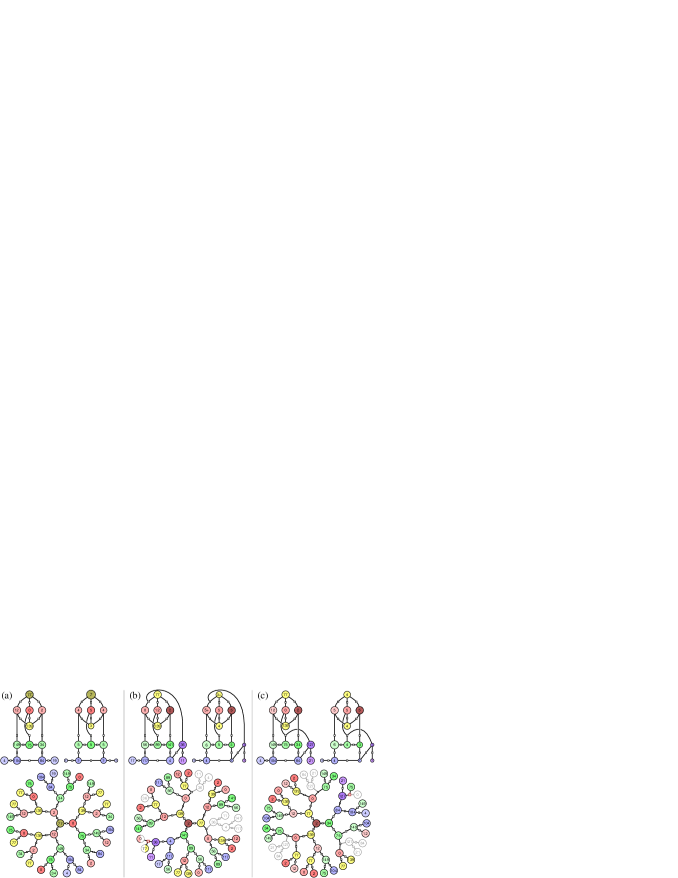
Figure 1: Parts of the full Tanner graph with nonzero noise for the instantons, corresponding to (a) simple, (b) degenerate and (c) sign-alternating pseudo-codewords, are shown in three panels each consisting of three diagrams. Bits are numbered according to the $(155,64,20)$-code definition (top left and bottom) and the noise level (top right, where the area of a bit/circle is proportional to the corresponding number). For the computational tree (bottom panel) the bits drawn in color participate in the pseudo-codeword and the shaded bit marks the error position. The marked checks/squares correspond to the points of (b) degeneracy and of (c) sign-alternation.

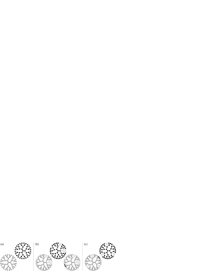
Figure 2: Interpretation of the instanton as a median within a set of pseudo-codewords. Three panels show the set of pseudo-codewords for the three instantons described in Fig. 1. Bits on the computational tree painted in white/black correspond to $+1/-1$. Other notations/marks are in accordance with the captions of Fig. 1.

Interpretation of the instantons found. The remarkable integer/rational structure of the instantons found numerically by “amoeba” admits a theoretical explanation. Our algebraic construction generalizes the computational tree approach of Wiberg 96Wib . The computational tree is built by unwrapping the Tanner graph of a given code into a tree from a bit for which we would like to determine the probability of error. (The erroneous bit is shaded in Fig. 1.) The number of generations in the tree is equal to the number of BP iterations (for more details see 95WLK ). As observed in 96Wib , the result of decoding at the shaded bit of the original code is exactly equal to the decoding result in the tree center. It should be noted that once magnetic fields representing an instanton are distributed on the tree, one can verify directly (by propagating messages from the leaves to the tree center) that the algorithm produces zero magnetization at the tree center. Any check node processes messages coming from the tree periphery in the following way: (i) the message with the smallest absolute value (we assume no degeneracy in the beginning) is passed, (ii) the source bit of the smallest message is colored, and (iii) the sign of the product of inputs is assigned to the outcome. At any bit that lies on the colored leaves-to-center path the incoming messages are summed up. The initial messages at any bit of the tree are magnetic fields and, therefore, the result obtained in the tree center is a linear combination of the magnetic fields with integer coefficients. The integer $n_{i}$ corresponding to bit $i$ of the original graph is the sum of the signatures over all colored replicas of $i$ on the computational tree. Therefore, the condition at the tree center becomes $\sum_{i}n_{i}h_{i}=0$. Returning to the original graph and maximizing the integrand of Eq. (2) with the condition enforced we arrive at the following expressions for the instanton configuration and the effective weight, respectively:

$$\varphi_{j}\!=\!n_{j}\Big{(}\sum_{i}n_{i}\Big{)}\Big{/}\Big{(}\sum_{i}n_{i}^{2}\Big{)},\quad l^{2}\!=\!\Big{(}\sum_{i}n_{i}\Big{)}^{2}\Big{/}\Big{(}\sum_{i}n_{i}^{2}\Big{)},$$ (3)

where the equation applies to the Gaussian channel, however its generalizations to any other channel is straightforward. One can check directly (e.g. looking at Fig. 1A) that Eqs. (3) are satisfied for the minimum weight instanton. In this case we find that the signature of any colored message before and after processing through a check remains intact, and thus the resulting $n_{i}$ for any colored bit is just a total number of the bit’s replicas. The structure of this instanton is exactly equivalent to one of the codewords on the computational tree, called a pseudo-codeword as generically it does not correspond to a codeword on the original graph 96Wib . However, Eq. (3) also suggests another possibility that goes beyond the standard pseudo-codeword construction 96Wib . In the case shown in Fig. 1C the colored part of the tree does correspond to a pseudo-codeword (by structure), however the pale part of the computational tree cannot be neglected as the noise values at these nodes are nonzero. This peculiarity is due to the fact that some of the checks shown in the upper part of Fig. 1C are connected to more than two colored bits. One finds that the signature of the message propagating from bit “75” to bit “127” alternates because of the pale “0” lying on a leaf, $8/47=|h_{0}|>|h_{75}|=3/47$, $h_{0}=-8/47<0$. This modifies $n_{75}$ making it equal to $4$, as one of the $6$ replicas of the bit “75” contributes to the total count $-1$ instead of $+1$. Moreover, looking at Fig. 1B one finds that the instanton can be even more elaborate as the number of replicas for some bits becomes fractional. (“+”-sign on Fig. 1B corresponds to $+7/18$.) This is actually the degenerate case with a colored structure bifurcating at a check (connected to the bits “0”,“77” and “36”) so that the messages entering the check from two distinct periphery have different signatures but are exactly equal to each other by the absolute value, $h_{0}=-h_{77}=18/79$. Eq. (3) does not work for this case, but the following generalization corrects the problem: one needs to introduce an additional condition accounting for the degeneracy. In our example this extra condition can be simply stated as $h_{0}=-h_{77}$. (See Appendix A Fig. S6.)

Instantons also allow for a complementary interpretation. A decoding error occurs when the magnetization in the computational tree center, which can be considered as a sum over all pseudo-code words weighted by, $\exp\left(s^{2}\sum_{i}h_{i}p_{i}\right)$, turns to zero (with $p_{i}$ being the number of bit $i$ replicas with $-1$ sign in the pseudo-codeword). In the case of high SNR (large magnetic fields) the sum is dominated by the pseudo-codewords of maximal weight. Therefore, any instanton, as a configuration of magnetic fields, should be equidistant from some set of $k\geq 2$ pseudo-codewords: $\sum_{i}h_{i}p^{(1)}_{i}=\dots=\sum_{i}h_{i}p^{(k)}_{i}$, where at least one of them has $+1$ value and at least one has $-1$ value in the tree center to achieve zero magnetization. And indeed the set of relevant pseudo-codewords for the $(155,64,20)$ code example, shown in Fig. 2, is a pair in the cases (a), (c) and a triple in the case (b). (See Appendixes.)

To conclude, in this Letter we demonstrated that the instanton approach is a very powerful, practical and generic instrument for quantitative analysis of the error floor. The success makes us confident that this novel method will be indispensable for future design of good and practical error-correcting schemes.

The authors acknowledge very useful and inspiring discussions with participants of workshop on “Applications of Statistical Physics to Coding Theory” sponsored by Los Alamos National Laboratory that took place January 10–12, 2005 in Santa Fe, NM, USA. This work was supported in part by DOE under LDRD program at Los Alamos National Laboratory, by the NSF under Grants CCR-0208597 and ITR-0325979 and by the INSIC.

Appendix A Appendix A: Supplementary Figures

Figure S1. Parity check matrix $\hat{H}$ for the $(155,64,20)$ LDPC code. The matrix consists of $3\times 5$ blocks. Each block is a square $31\times 31$ matrix. Empty/filled elements of the matrix stand for $0/1$. Bits are numbered from “0” to “154”. The girth of this code is eight.

Figure S2. Frame-Error-Rate (FER) vs SNR² for the $(155,64,20)$ code and Belief Propagation decoding. The filled/empty circle-marks correspond to result of Monte Carlo evaluation of FER for $4/1024$ iterations of BP. The straight/dashed line corresponds to the (a)-instanton asymptotic, $\sim\exp[-(46^{2}/210)\cdot s^{2}/2]$ and the ML asymptotic, $\sim\exp[-20\cdot s^{2}/2]$.

Figure S3. Min-sum decoding for the (a) instanton on the computational tree. All numbers are in units of $1/105$. The numbers shown on the bits/circles are the values of the magnetic fields, $h$. The number shown next to each check/square is the message, $\eta$, arriving at the check on the $q$-th step of the iteration procedure, where $4-q$ corresponds to the number of bits separating this check from the tree center. Other notations/marks are in accordance with the caption of Fig. 1 of the main text.

Figure S4. Min-sum decoding for the (b) instanton on the computational tree. All numbers are in units of $1/79$. Other notations/marks and explanations are in accordance with captions of Fig. 1 of the main text and Fig. S3.

Figure S5. Min-sum decoding for the (c) instanton on the computational tree. All numbers are in the units of $1/47$. Other notations/marks and explanations are in accordance with captions of Fig. 1 of the main text and Fig. S3.

Figure S6. Geometrical interpretation of the degeneracy observed in case (b). The plot shows distance $l^{2}$ for the noise configuration in case (b), minimized with respect to all the magnetic fields except $h_{0}$ and $h_{77}$, vs the two remaining fields. The relevant part of the $(h_{0},h_{77})$ plane is the quadrant $h_{0}<0$, $h_{77}>0$. Looking for the instanton in the $|h_{0}|<|h_{77}|$ domain and thus assuming that the “0” bit connected to the red check in Fig. 1B of the main text is colored while bit “77” is pale, one gets the paraboloid, shown in pink in the Figure, that achieves its minimum outside of the domain, i.e. in the $|h_{0}|>|h_{77}|$ semi-quadrant. Similarly, if one looks for the instanton in the $|h_{0}|>|h_{77}|$ domain one again finds an inconsistency as the respective paraboloid, shown in yellow in the Figure achieves its minimum in the $|h_{0}|<|h_{77}|$ semi-quadrant. Therefore, the point of actual minimum, shown by the green dot on the Figure, lies exactly at the minimum of the angled join of the two domains, $|h_{0}|=|h_{77}|$.

Appendix B Appendix B: Instantons for the min-sum decoding

These notes consist of three parts. The first part is devoted to explaining how the entire instanton family for an arbitrary LDPC code decoded by the min-sum algorithm can be fully characterized using the computational tree approach. The second part describes an alternative exposition which allows one to represent an instanton as a configuration of magnetic fields equidistant from some set of codewords on the computational tree. The third part formulates a relation between the theoretical and numerical approaches and suggests challenges and questions that need to be addressed in the future.

B.1 Colored/signature structure and constraint minimization

The basic object for our construction is the computational tree and its colored/pale/uncolored parts (as briefly introduced in the main text). The computational tree is a tree constructed by a simple unwrapping of the Tanner graph of the code into a tree starting from the bit where the BER is calculated. The number of generations on the tree is equal to the number of iterations of the decoder, $n_{\rm it}$. If $n_{\rm it}$ is larger than, or equal to, a quarter of the code girth (defined as the length of the shortest loop of the original Tanner graph, measured by the number of edges within the loop), then the computational tree contains more than one replica of some of the bits of the original code.

Consider an arbitrary configuration of magnetic field, ${\bm{h}}$ (or noise field, ${\bm{\varphi}}$) on the Tanner graph, and on the computational tree respectively. Calculating the magnetization (or switching from physics jargon to communication theory jargon, a-posteriori log-likelihood) at the $n_{\rm it}$-th iteration in the center of the tree one derives, $m^{(n_{\rm it})}_{\rm center}={\bm{h}}\cdot{\bm{n}}$. $n_{i}$, defined on a bit of the original Tanner graph is an integer. It is a sum of contributions, each originating from the respective bit/replica on the computational tree. Colored are bits on the tree that contribute the integer $+1$ or $-1$. (In the Figures of the main text and Supporting Figures we use different colors to identify bits in the computational tree originating from different bits of the original Tanner graph.) A colored bit on the computational tree has the signature $+1/-1$ if it contributes $+1/-1$ to the integer associated with the respective bit on the Tanner graph. Uncolored bits (i.e. bits not shown in the Figures) or pale bits (i.e. bits shown pale in the Figures) on the tree do not contribute to the respective integer (one may also say that the respective contribution is just zero) according to the min-part of the min-sum rules described in Eq. (1) of the main text. We draw a bit on the computational tree in pale if it does not contribute to respective integer, however at least one of its siblings, i.e. bits on the tree originating from the same bit on the computational tree, does contribute to the integer.)

Let us now describe how an individual contribution of a colored bit on the tree to the respective integer (that is $+1$ or $-1$) is calculated. We aim to calculate the contribution to magnetization at the tree center counting integers according to the min-sum rule. We assign $+1$ signatures to the colored leaves of the tree and start an iterative procedure which assigns signatures moving from the tree leaves towards the tree center. Consider the case when at a certain step of the iteration procedure a check receives messages from some number of bits among which only one is colored. Then one calculates the product of the signatures associated with the messages this check receives from the remaining bits. If the resulting product is $+1/-1$ the signature of the colored bit is $+1/-1$ and the signatures of the colored bits, laying on the tree branch grown from the given colored bit, do not/do change. The other possibility (that will be called degenerate) is that a check receives two (or more) messages that all have the same absolute value, which is also the minimal of all the messages received. Then, one has the freedom to color only one of the degenerate bits with a colored branch grown from it with the signatures assigned as described above. The iterative procedure of the signature assignment is terminated once the three center is reached. One calls a check marked if it lies in between two colored bits of different signatures.

The union of all colored bits, i.e. bits contributing to $m^{(n_{\rm it})}_{\rm center}$, is called the colored structure. Any check connected to the colored structure is actually connected to two bits of the structure. Another important characteristic complementing the notion of the colored structure on the computational tree is the set of aforementioned signatures $\pm 1$ associated with any bit of the colored structure. In a degenerate case, one finds multiple colored/signature structures associated with a given configuration of magnetic fields. Each degenerate structure will actually correspond to a distinct linear combination of magnetic fields equal to $m^{(n_{\rm it})}_{\rm center}$. Therefore, of the whole variety of possible degenerate colored/signature structures corresponding to the same magnetic field one can always select a set of linearly independent ones.

So far, this description was generic, i.e. not restricted to a specific configuration of the magnetic field. Let us now fix the family of linear independent colored/signature structures just explained and allow variation in the value of magnetic fields. Our goal here is to find an instanton conditioned to the specific form of the family of the linear independent colored/signature structures. Finding the instanton means minimizing $l^{2}=({\bm{1}}-{\bm{h}})^{2}$ with respect to ${\bm{h}}$ under the additional set of linearly independent conditions, $m^{(n_{\rm it})}={\bm{h}}\cdot{\bm{n}}^{(\mu)}=0$, where $\mu$ is an index enumerating these conditions each corresponding to a certain colored structure. (The expression presented above for the length $l$ applies to the white Gaussian channel, however generalization for any other channel is straightforward.) The resulting expression for the optimal configuration of the noise, ${\bm{\varphi}}={\bm{1}}-{\bm{h}}$, is

$${\bm{\varphi}}=\sum_{\mu,\nu}{\bm{n}}^{(\mu)}(\hat{G}^{-1})_{\mu\nu}\sum_{i}n_{i}^{(\nu)},\quad G_{\mu\nu}\equiv{\bm{n}}^{(\mu)}\cdot{\bm{n}}^{(\nu)}.$$ (S1)

This expression (also generalizing Eq. (3) of the main text for an arbitrary type of instanton degeneracy) should be checked for consistency with the family of the colored/signature structures assumed for the instanton. If the consistency check is met, the instanton construction is completed.

Let us now demonstrate how this formal description works for the three instanton examples (a), (b) and (c) described in Figs. 1, 2 of the main text and also illustrated in Figs. S3–S6. Instantons (a) and (c) are both explained by a single colored structure. For the (a) instanton each bit contributes $+1$ to the respective component of ${\bm{n}}$. For the (c) example all contributions are $+1$ except of the one coming from the “75” bit connected to the marked check. Since $h_{0}<0$, the message originating from this bit contributes with the opposite sign to the magnetization. There exist $6$ replicas of the “75” bit on the computational tree, however taking into account that one replica of the bit contributes $-1$, one finds that the actual value of the noise is $\sim 4$ rather than $\sim 6$. Since $|h_{0}|>|h_{75}|$, the “0” bit is pale thus it does not contribute to the magnetization. Considering the (b) instanton one finds that this is a degenerate example, with $|h_{0}|=|h_{77}|$. There are two linearly independent colored/signature structures describing the (b) instanton. The two structures are different only at the two bits on the tree leaves shown in Fig. 1B of the main text adjusted to the marked check. The first colored structure does not contain bit “77” (zero contribution to the magnetization) while bit “0” contributes $+1$ to the respective component of ${\bm{n}}$. The second structure does not contain bit “0” while bit “77” contributes $-1$ to the respective component of ${\bm{n}}$ (simply because $h_{0}<0$, thus forcing the respective message to contribute to the magnetization with the opposite sign).

One natural question to ask about the degenerate case (b) is the following: can one of the two colored structures describing the instanton be forming its own non-degenerate instanton? The answer is negative. Indeed, the colored/signature structure generates (through the minimization procedure described above) such a configuration of magnetic fields that will not be consistent with the colored/signature structure one started from. Considering the structure with the “0” bit connected to the marked check being pale (and thus the signature field associated with the colored bit “77” connected to the red check being $-1$) one finds that the magnetic field minimizing $l$ will actually be inconsistent with the colored/signature structure. Considering the other configuration (the “0” bit is colored with $+1$ signature while the “77” bit is pale) one finds again that the resulting magnetic field is inconsistent with the colored structure. To resolve this inconsistency one needs to account for the two configurations simultaneously, thus introducing two constraints, not one. The degeneracy of the (b) instanton is illustrated in Fig. S6.

Let us also notice that the discrete nature of consistency check (yes/no answer as a result) puts degenerate configurations on equal footing (in the sense of counting all possibilities) with the non-degenerate configurations: considering the family of all possible instantons for the given computational tree one finds that the number of degenerate instantons is comparable with the number of nondegenerate instantons.

B.2 Instantons as medians between pseudo-codewords

We consider an instanton with the set of linearly independent structures already established. Each colored structure, indexed by $\mu$, corresponds to the constraint, ${\bm{h}}\cdot{\bm{n}}^{(\mu)}=0$, imposed on the magnetic field, ${\bm{h}}$. Each of the constraints can actually be reformulated in terms of a pair of pseudo-codewords on the computational tree:

$$\sum\limits_{i\in{\rm tree}}h_{i}\sigma_{i}^{(\mu;+)}=\sum\limits_{i\in{\rm tree}}h_{i}\sigma_{i}^{(\mu;-)},$$ (S2)

where $i$ stands for index assigned to a bit on the computational tree; the magnetic field on the computational tree bit is equal to the magnetic field defined on the respective bit of the original graph; and the pseudo-codewords, ${\bm{\sigma}}^{(\mu;\pm)}$, are the two distinct configurations of the binary field, $\sigma_{i}=\pm 1$, defined on each bit $i$ of the computational tree that satisfy all the checks on the computational tree.

Let us now discuss how the pseudo-codewords can be constructed if the respective constraint $\mu$ described by Eq. (S2), is already established. If the signature field, described in the previous Section of the Notes, corresponding to the structure $\mu$, does not contain a single $-1$ element, then ${\bm{\sigma}}^{(\mu;+)}$ is the all unity codeword ($+1$ on all bits of the computational tree) and ${\bm{\sigma}}^{(\mu;-)}$ is the pseudo-codeword containing $-1$ on all the colored bits of the structure and $+1$ on all other bits. If, however, the colored structure does contain some $-1$ signatures the situation is more elaborate as both pseudo-codewords are nontrivial. The algorithm that allows restoration of the pseudo-code words starts by determining the values of the colored bits for ${\bm{\sigma}}^{(\mu;+)}$ that are set equal to the values of the signatures. The uncolored bits are assigned values $+1$. Although it is possible to determine the bit values of the pale substructures the procedure is elaborate and we are not presenting it here. Finally, the pseudo-codeword ${\bm{\sigma}}^{(\mu;-)}$ is obtained from ${\bm{\sigma}}^{(\mu;+)}$ by changing the signs of colored bits with the uncolored and pale bits remaining the same.

Fig. 2 of the main text shows three examples of the pseudo-codeword construction for the three instantons discussed in the manuscript. Examples (a), (c) contain one pair of competing pseudo-codewords. However, the two cases are different. In the case (a) the colored/signature structure does not contain $-1$ bits, thus one pseudo-codeword is just the all unity codeword and another pseudo-codeword contains $-1$ at all the bits of the colored structure and $+1$ at all other bits. In the (c) case the colored/signature structure does contain $-1$ bit thus resulting in two distinct pseudo-codewords shown in Fig. 2C of the main text. Example (b) corresponds to the degenerate case with the two pairs of pseudo-codewords involved in the conditions (S2). However, one pseudo-codeword enters both conditions (that is the one shown on the top diagram of Fig. 2B of the main text) therefore the total count for the case (b) gives three pseudo-codewords being equidistant from the instanton configuration of the magnetic fields.

B.3 General Remarks

Let us note that the analysis presented above, in addition to its theoretical significance, may be helpful for accelerating the instanton-amoeba numerical procedure, e.g. through guiding selection on the final stage of the minimization. We also expect that this theoretical analysis will be instrumental for formulating the right questions to address by the instanton-amoeba method, or by other minimization methods aiming at finding the instanton numerically. In what follows, we conclude by posing some questions that we did not yet study but plan to address in the future.

• More detailed exploration of the phase space, especially in the context of describing not only the minimal distance $l_{\rm min}$ contribution but also the family of other “low laying” instantons. The particular question of interest here is to estimate the “density of states/instantons”, that is to answer the question: how many instantons are found within the $\delta l$ vicinity of the one correspondent to $l_{\rm min}$?

• Dependence of BER on the number of iterations. As we already indicated in the main text our preliminary tests show that instantons and thus asymptotic estimates for BER do change with the number of iterations. We will be interested to explain this dependence. We will also be testing with our instanton-amoeba approach, the validity of the graph covers method suggested recently 03KV .

• Dependence on the code length. It is important to analyze the family of LDPC codes with varying code length, $N$. Of a special interest are the regular LDPC codes where the Hamming distance grows with $N$, e.g. Margulis codes 82Mar . Then, the relevant question is: how does $l_{\rm min}$ (and other characteristics of the error floor) change with $N$ for a given family of codes? This study will essentially lead to analysis of the finite-size effects, already discussed in the water-fall domain 04ARMR , but not yet explored in the asymptotic regime of the error-floor.

• Does BP/min-sum decoding perform better than other suboptimal algorithms (that can possibly exist) of the same complexity, e.g. linear in $N$? Even if the answer is yes (that is by no means guaranteed), what would be the best decoding for a higher level of complexity, e.g. $N^{a}$, where $a>1$? Once an idea of better decoding is formulated, our instanton-amoeba toolbox will be indispensable in answering the aforementioned questions and also testing in depth the performance of the new decoding.

• Other types of codes, e.g. turbo codes. Turbo codes show remarkable performance at moderate SNR but they are also infamous for demonstrating much higher (than comparable in size LDPC codes) error floors. Even though some important similarities between the LDPC codes and turbo codes are established 98MMC , the decoders of these two types of codes are different and it becomes important to analyze the performance of the turbo scheme, especially in light of the turbo-codes popularity.

• Other, application specific, channels. The instanton-amoeba approach is not limited to the white Gaussian channel, which we choose primarily for the purpose of demonstration, but can be applied straightforwardly to other types of channels, e.g. with correlations among received samples. Of special interest will be to analyze the performance of fiber-optic communication channels where the effects of fiber dispersion 03CCDGKL , birefringence and amplifier noise 04CCGKL will be accounted for. Another two interesting channel types are magnetic and optical recording channels exhibiting high level of nonlinearity and correlations among received samples 04BV_book .

• There are many problems in the information and computer sciences that are different from standard coding problem but are also dependent or sensitive to rare errors. Therefore, estimating performance/BER in these problems is a major step required for their comprehensive analysis. Two interesting examples here are (i) inter-symbol interference, that is especially challenging in the context of two-dimensional 03WOSI and three-dimensional information storage, and (ii) estimating algorithmic errors in the domain of typically good performance within a combinatorial optimization K-SAT setting 02MPZ .

References

- (1) R.G. Gallager, Low density parity check codes (MIT Press, Cambridge, 1963).
- (2) C. Berrou, A. Glavieux, P. Thitimajshima, Near Shannon limit error-correcting coding and decoding: turbo codes, Proceedings IEEE International Conference on Communications, 23–26 May 1993, Geneva, Switzerland; vol. 2, pp. 1064–70.
- (3) D.J.C. MacKay, Good error-correcting codes based on very sparse matrices, IEEE Trans. Inf. Theory 45, 399–431 (1999).
- (4) C.E. Shannon, A mathematical theory of communication, Bell Syst. Tech. J. 27, 379–423 (1948).
- (5) D.J.C. MacKay, M.S. Postol, Weaknesses of Margulis and Ramanujan-Margulis low-density parity-check codes, Electronic Notes in Theoretical Computer Science 74, 1–8 (2003).
- (6) T. Richardson, Error floors of LDPC codes, 2003 Allerton conference Proccedings.
- (7) A.A. Belavin, A.M. Polyakov, A.S. Schwartz, Y.S. Tyupkin, Pseudoparticle solutions of Yang-Mills equations, Phys. Lett. B 59, 85–87 (1975).
- (8) I.M. Lifshitz, Energy spectrum structure and quantum states of disodered condensed systems, Usp. Fiz. Nauk 83, 617 (1964) [Sov. Phys. Usp. 7, 549–573 (1965)].
- (9) T. Richardson, R. Urbanke, The renaissance of Gallager’s low-density parity-check codes, IEEE Communications Magazine 41, 126–131 (2003).
- (10) B. Vasic, O. Milenkovic, Combinatorial construction of low-density parity check codes, IEEE Trans. Inf. Theory, 50, 1156–1176 (2004).
- (11) N. Wiberg, H-A. Loeliger, R. Kotter, Codes and iterative decoding on general graphs, Europ. Transaction Telecommunications 6, 513–525 (1995).
- (12) N. Wiberg Codes and decoding on general graphs, Ph.D. thesis, Linköping University, 1996.
- (13) G.D. Forney Jr., R. Koetter, F.R. Kschischang, A. Reznik, On the effective weights of pseudocodewords for codes defined on graphs with cycles, IMA Volumes in Mathematics and its Applications 123, 101–112 (2001).
- (14) Y. Weiss, W.T. Freeman, On the optimality of the max-product belief propagation algorithm in arbitrary graphs, IEEE Trans. Inf. Theory 47, 736–744 (2001).
- (15) F.R. Kschischang, B.J. Frey, H.A. Loeliger, Factor graphs and the sum-product algorithm, IEEE Trans. Inf. Theory 47, 498–519 (2001).
- (16) N. Sourlas, Spin-glass models as error-correcting codes, Nature (London) 339, 693–695 (1989).
- (17) A. Montanari, The glassy phase of Gallaher codes, Eur. Phys. J. B 23, 121–136 (2001).
- (18) J.S. Yedidia, W.T. Freeman, Y. Weiss, Constructing Free Energy Approximations and Generalized Belief Propagation Algorithms, TR-2002-35, http://www.merl.com/reports/TR2002-35/index.html .
- (19) M. Mezard, Passing messages between disciplines, Science 301, 1685 (2003).
- (20) S. Benedetto, G. Montorsi, Unveiling turbo codes:results concatenated coding schemes, IEEE Trans. Inf. Theory 42, 409–428 (1996).
- (21) Y. Mao, A.H. Banihashemi, A heuristic search for good low-density parity-check codes at short block lengths, Proc. IEEE Int. Conf. Communications 1, 41–44 (2001).
- (22) T. Tian, C. Jones, J. Villasenor, R.D. Wesel Construction of irregular ldpc codes with low error foors, Proc. IEEE Int. Conf. Communications 5, 3125–3129 (2003).
- (23) C. Di, D. Proietti, I.E. Telatar, T.J. Richardson, R.L. Urbanke, Finite-length Analysis of Low Density Parity Check Codes on the Binary Erasure Channel, IEEE Trans. Inf. Theory 48, 1570–1579 (2002).
- (24) P.O. Vontobel, R. Koetter, Lower bounds on the minimum pseudo-weight of linear codes, Proceedings of IEEE International Symposium on Information Theory, Chicago, IL, Jun./Jul. 2004, p.70.
- (25) H.A. Bethe, Statistical theory of superlattices, Proc. Roy. Soc. London A 150, 552–575 (1935).
- (26) W.H. Press et al. Numerical recipes in C: the art of scientific computing (Cambridge University Press, 1988).
- (27) V. Chernyak, M. Chertkov, M.G. Stepanov, B. Vasic, Error correction on a tree: an instanton approach, Phys. Rev. Lett. 93, 198702 (2004).
- (28) R.M. Tanner, D. Srkdhara, T. Fuja, A Class of Group-Structured LDPC Codes, Proc. of ICSTA 2001, Ambleside, England.
- (29) R. Koetter, P.O. Vontobel, Graph covers and iterative decoding of finite-length codes, Proc. 3rd International Symposium on Turbo Codes & Related Topics, Brest, France, p. 75–82, Sept. 1-5, 2003.
- (30) G.A. Margulis, Explicit construction of graphs without short circles and low-density codes, Combinatorica 2, 71–78 (1982).
- (31) A. Abdelaziz, R. Urbanke, A. Montanari, T. Richardson, Further results on finite-length scaling for iteratively decoded LDPC ensembles, Proc. IEEE 2004 International Symposium on Information Theory, p. 103. See also http://arxiv.org/abs/cs/0406050.
- (32) R.J. McEliece, D.J.C. MacKay, J.F. Cheng, Turbo decoding as an instance of Pearl’s “belief propagation” algorithm, IEEE J. Select. Areas Commun. 16 140–152 (1998).
- (33) M. Chertkov,Y. Chung, A. Dyachenko, I. Gabitov, I. Kolokolov, V. Lebedev, Shedding and interaction of solitons in weakly disordered optical fibers, Phys. Rev. E 67, 036615 (2003).
- (34) M. Chertkov, V. Chernyak, I. Gabitov, I. Kolokolov, V. Lebedev, PMD induced fluctuations of Bit-Error-Rate in optical fiber systems, Journal of Lightware Technology 22, 1155–1168 (2004).
- (35) B. Vasic, E.M. Kurtas (editors) Coding and Signal Processing for Magnetic Recording Systems (CRC Press, New York, 2004).
- (36) Y. Wu, J.A. O’Sullivan, N. Singla, R.S. Indeck, Iterative detection and decoding for separable two-dimensional intersymbol interference, IEEE Transactions on Magnetics 39, 2115–2120 (2003).
- (37) M. Mezard, G. Parisi, R. Zecchina, Analytic and algorithmic solution of random satisfiability problems, Science 297, 812–815 (2002).