Fundamental aspects of electron correlations and quantum transport in one-dimensional systems

Abstract

Some aspects of physics on interacting fermions in 1D are discussed in a tutorial-like manner. We begin by showing that the non-analytic corrections to the Fermi-liquid forms of thermodynamic quantities result from essentially 1D collisions embedded into a higher-dimensional phase space. The role of these collisions increases progressively as dimensionality is reduced until, finally, they lead to a breakdown of the Fermi liquid in 1D. An exact solution of the Tomonaga-Luttinger model, based on the Ward identities, is reviewed in the fermionic language. Tunneling in a 1D interacting systems is discussed first in terms of the scattering theory for interacting fermions and then via bosonization. Universality of conductance quantization in disorder-free quantum wires is discussed along with the breakdown of this universality in the spin-incoherent case. A difference between charge (universal) and thermal (non-universal) conductances is explained in terms of Fabry-Perrot resonances of charge plasmons.

1 Introduction

The theory of interacting fermions in one dimension (1D) has survived several metamorphoses. From what seemed to be a purely mathematical exercise up until the 60s, it had evolved into a practical tool for predicting and describing phenomena in conducting polymers and organic compounds–which were the 1D systems of the 70s. Beginning from the early 90s, when the progress in nanofabrication led to creation of artificial 1D structures–quantum wires and carbon nanotubes, the theory of 1D systems started its expansion into the domain of mesoscopics; this trend promises to continue in the future. Given that there is already quite a few excellent reviews and books on the subject [1]-[10] , I should probably begin with an explanation as to what makes this review different from the others. First of all, it is not a review but–being almost a verbatim transcript of the lectures given at the 2004 Summer School in Les Houches–rather a tutorial on some (and definitely not all) aspects of 1D physics. A typical review on the subject starts with describing the Fermi Liquid (FL) in higher dimensions with an aim of emphasizing the differences between the FL and its 1D counter-part –Luttinger Liquid (LL). My goal–if defined only after the manuscript was written–was rather to highlight the similarities between higher-D and 1D systems. The progress in understanding of 1D systems has been facilitated tremendously and advanced to a greater detail, as compared to higher dimensions, by the availability of exact or asymptotically exact methods (Bethe Ansatz, bosonization, conformal field theory), which typically do not work too well above 1D. The downside part of this progress is that 1D effects, being studied by specifically 1D methods, look somewhat special and not obviously related to higher dimensions. Actually, this is not true. Many effects that are viewed as hallmarks of 1D physics, e.g., the suppression of the tunneling conductance by the electron-electron interaction and the infrared catastrophe, do have higher-D counter-parts and stem from essentially the same physics. For example, scattering at Friedel oscillations caused by tunneling barriers and impurities is responsible for zero-bias tunneling anomalies in all dimensions [11, 16]. The difference is in the magnitude of the effect but not in its qualitative nature. Following the tradition, I also start with the FL in Sec. 2, but the main message of this Section is that the difference between $D=1$ and $D>1$ is not all that dramatic. In particular, it is shown that the well-known non-analytic corrections to the FL forms of thermodynamic quantities (such as a venerable $T^{3}\ln T$-correction to the linear-in-$T$ specific heat in 3D) stem from rare events of essentially 1D collisions embedded into a higher-dimensional phase space. In this approach, the difference between $D=1$ and $D>1$ is quantitative rather than qualitative: as the dimensionality goes down, the phase space has difficulties suppressing the small-angle and $2k_{F}-$scattering events, which are responsible for non-analyticities. The special point when these events go out of control and start to dominate the physics happens to be in 1D. This theme is continued in Sec.5, where scattering from a single impurity embedded into a 1D system is analyzed in the fermionic language, following the work by Yue, Matveev, Glazman [11]. The drawback of this approach–the perturbative treatment of the interaction–is compensated by the clarity of underlying physics. Another feature which makes these notes different from the rest of the literature in the field is that the description goes in terms of the original fermions for quite a while (Secs.2 through 5) , whereas the weapon of choice of all 1D studies–bosonization– is invoked only at a later stage (Sec. 6 and beyond). The rationale–again, a post-factum one–is two-fold. First, 1D systems in a mesoscopic environment–which are the main real-life application discussed here– are invariably coupled to the outside world via leads, gates, etc. As the outside world is inhabited by real fermions, it is sometimes easier to think of, e.g., both the interior and exterior a quantum wire coupled to reservoirs in terms of the same elementary quasi-particles. Second, after 40 years or so of bosonization, what could have been studied within a model of fermions with linearized dispersion and not too strong interaction–and this is when bosonization works–was probably studied. (As all statements of this kind, this is one is also an exaggeration.) The last couple of years are characterized by a growing interest in either the effects that do not occur in a model with linearized dispersion, e.g., Coulomb drag due to small-momentum transfers [17] and energy relaxation, or situations when strong Coulomb repulsion does not permit linearization of the spectrum at any energies [19, 20, 21]. Experiment seems to indicate that the Coulomb repulsion is strong in most systems of interest, thus studies of a strongly-coupled regime are quite timely. Once the assumption of the linear spectrum is abandoned, the beauty of a bosonized description is by and large lost, and one might as well come back to original fermions. Sec.6 is devoted to transport in quantum wires, mostly in the absence of impurities. The universality of conductance quantization is explained in some detail, and is followed by a brief discussion of the recent result by Matveev [19], who showed that incoherence in the spin sector leads to a breakdown of the universality at higher temperatures (Sec. 7.4). Also, a difference in charge (universal) and thermal (non-universal) transport–emphasized by Fazio, Hekking, and Khmelnitskii [22]– in addressed in Sec.7.5. What is missing is a discussion of transport in a disordered (as opposed to a single-impurity) case. However, this canonically difficult subject, which involves an interplay between localization and interaction, is perhaps not ready for a tutorial-like discussion at the moment. (For a recent development on this subject, see Ref.[18].)

Even a brief inspection of these notes shows that the choice between making them comprehensive or self-contained was made for the latter with a focus on a relatively small number of topics. It is quite easy to see what is missing: there is no discussion of lattice effects, bosonization is introduced without the Klein factors, the sine-Gordon model is not treated in depth, chiral Luttinger liquids are not discussed at all, and the list goes on. The discussion of the experiment is scarce and perfunctory. However, the few subjects that are discussed are provided with quite a detailed–perhaps somewhat excessively detailed– treatment, so that a reader may not feel a need to consult the reference list too often. For the same reason, the notes also cover such canonical procedures as the perturbative renormalization group in the fermionic language (Sec. 4) and elementary bosonization (Sec. 6), which are discussed in many other sources and a reader already familiar with the subject is encouraged to skip them.

Also, a relatively small number of references (about one per page on average) indicates once again that this is not a review. The choice of cited papers is subjective and the reference list in no way pretends to represent a comprehensive bibliography to the field. My apologies in advance to those whose contributions to the field I have failed to acknowledge here.

$\hbar=k_{B}=1$ through out the notes, unless specified otherwise.

2 Non-Fermi liquid features of Fermi liquids: 1D physics in higher dimensions

One often hears the statement that, by and large, a Fermi liquid (FL) is just a Fermi gas of weakly interacting quasi-particles; the only difference being the renormalization of the essential parameters (effective mass, $g-$ factor) by the interactions. What is missing here is that the similarity between the FL and Fermi gas holds only for leading terms in the expansion of the thermodynamic quantities (specific heat $C(T)$, spin susceptibility $\chi_{s}$, etc.) in the energy (temperature) or spatial (momentum) scales. Next-to-leading terms, although subleading, are singular (non-analytic) and, upon a closer inspection, reveal a rich physics of essentially 1D scattering processes, embedded into a high-dimensional phase space.

In this chapter, I will discuss the difference between “normal” processes which lead to the leading, FL forms of thermodynamic quantities and “rare” 1D processes which are responsible for the non-analytic behavior. We will see that the role of these rare processes increases as the dimensionality is reduced and, eventually, the rare processes become the norm in 1D, where the FL breaks down.

In a Fermi gas, thermodynamic quantities form regular, analytic series as function of either temperature, $T,$ or the inverse spatial scale (bosonic momentum $q)$ of an inhomogeneous magnetic field. For $T\ll E_{F},$ where $E_{F}$ is the Fermi energy, and $q\ll k_{F},$ where $k_{F}$ is the Fermi momentum, we have

$$C(T)/T = \gamma+aT^{2}+bT^{4}+\dots;$$ (2.1a)

$$\chi_{s}\left(T,q=0\right) = \chi_{s}^{0}(0)+cT^{2}+dT^{4}+\dots;$$ (2.1b)

$$\chi_{s}\left(T=0,q\right) = \chi_{s}^{0}(0)+eq^{2}+fq^{4}+\dots,$$ (2.1c)

where $\gamma$ is the Sommerfeld constant, $\chi_{s}^{0}$ is the static, zero-temperature spin susceptibility (which is finite in the Fermi gas), and $a\dots f$ are some constants. Even powers of $T$ occur because of the approximate particle-hole symmetry of the Fermi function around the Fermi energy and even powers of $q$ arise because of the analyticity requirement

Our knowledge of the interacting systems comes from two sources. For a system with repulsive interactions, one can assume that as long as the strength of the interaction does not exceed some critical value, none of the symmetries (translational invariance, time-reversal, spin-rotation, etc.), inherent to the original Fermi gas, are broken. In this range, the FL theory is supposed to work. However, the FL theory is an asymptotically low-energy theory by construction, and it is really suitable only for extracting the leading terms, corresponding to the first terms in the Fermi-gas expressions (2.1a-2.1c). Indeed, the free energy of a FL as an ensemble of quasi-particles interacting in a pair-wise manner can be written as [25]

$$F-F_{0}=\sum_{k}\left(\epsilon_{k}-\mu\right)\delta n_{k}+\frac{1}{2}\sum_{k,k^{\prime}}f_{k,k^{\prime}}\delta n_{k}\delta n_{k^{\prime}}+O\left(\delta n_{k}^{3}\right),$$ (2.2)

where $F_{0}$ is the ground state energy, $\delta n_{k}$ is the deviation of the fermion occupation number from its ground-state value, and $f_{k,k^{\prime}}$ is the Landau interaction function. As $\delta n_{k}$ is of the order of $T/E_{F},$ the free energy is at most quadratic in $T,$ and therefore the corresponding $C(T)$ is at most linear in $T.$ Consequently, the FL theory–at least, in the conventional formulation–claims only that

$$C^{\ast}(T)/T = \gamma^{\ast};$$

$$\chi_{s}^{\ast}\left(T,q\right) = \chi_{s}^{\ast}\left(0\right),$$

where $\gamma^{\ast}$ and $\chi_{s}^{\ast}\left(0\right)$ differ from the corresponding Fermi-gas values, and does not say anything about higher-order terms .

Higher-order terms in $T$ or $q$ can be obtained within microscopic models which specify particular interaction and, if an exact solution is impossible–which is always the case in higher dimensions– employ some kind of a perturbation theory. Such an approach is complementary to the FL: the former nominally works for weak interactions but at arbitrary temperatures, whereas FL works both for weak and strong interactions, up to some critical value corresponding to an instability of some kind, e.g., a ferromagnetic transition, but only in the low-temperature limit. In the $\{$ temperature, interaction$\}$ plane, the validity regions of these two approaches are two strips running along the two axes (cf. Fig. 1). For weak interactions and at low temperatures, the regions should overlap.

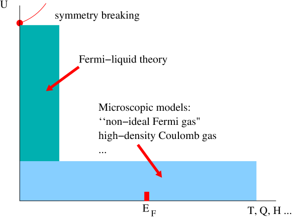
Fig. 1.: Combined “diagram of knowledge". x-axis: energy scale (given by temperature $T$, bosonic momentum $Q$, magnetic field $H$) in appropriate units. y-axis: interaction strength. Fermi liquid works for not necessarily weak interactions (but smaller than the critical value for an instability of the ground state denoted by the red dot) but at the lowest energy scales. Microscopic models work for weak interactions but for arbitrary energies.

Microscopic models (Fermi gas with weak repulsion, Coulomb gas in the high-density limit, electron-phonon interaction, paramagnon model, etc.) show that the higher-order terms in the specific heat and spin susceptibility are non-analytic functions of $T$ and $q$ [26, 27, 28, 29, 30, 31, 32, 33, 34, 35, 36, 37, 38]. For example,

$$C(T)/T = \gamma_{3}-\alpha_{3}T^{2}\ln T\text{{\ (3D);}}$$ (2.3a)

$$C(T)/T = \gamma_{2}-\alpha_{2}T\text{{\ (2D) ;}}$$ (2.3b)

$$\chi_{s}\left(q\right) = \chi_{s}(0)+\beta_{3}q^{2}\ln q^{-1}\text{{\ (3D);}}$$ (2.3c)

$$\chi_{s}\left(q\right) = \chi_{s}(0)+\beta_{2}\left|q\right|\,\text{{\ (2D),}}$$ (2.3d)

where all coefficients are positive for the case of repulsive electron-electron interaction

As seen from Eqs. (2.3a-2.3d), the non-analyticities become stronger as the dimensionality is reduced. The strongest non-analyticity occurs in 1D, where– as far as single-particle properties are concerned–the FL breaks down:

$$C(T)/T = \gamma_{1}+\alpha_{1}\ln T\text{{\ \ (1D);}}$$

$$\chi\left(q\right) = \chi_{0}+\beta_{1}\ln\left|q\right|\mathrm{\ \ (1D).}$$

It turns out that the evolution of the non-analytic behavior with the dimensionality reflects an increasing role of special, almost 1D scattering processes in higher dimensions. Thus non-analyticities in higher dimensions can be viewed as precursors of 1D physics for $D>1.$

It is easier to start with the non-analytic behavior of a single-particle property, the self-energy, which can be related to the thermodynamic quantities via standard means [23] (see also appendix A). Within the Fermi liquid,

$$\mathrm{Re}\Sigma^{R}\left(\varepsilon,k\right) = -A\varepsilon+B\xi_{k}+\dots$$ (2.4a)

$$-\mathrm{Im}\Sigma^{R}\left(\varepsilon,k\right) = C(\varepsilon^{2}+\pi^{2}T^{2})+\dots$$ (2.4b)

Expressions (2.4a) and (2.4b) are equivalent to two statements: i) quasi-particles have a finite effective mass near the Fermi level

$$m^{\ast}=m_{0}\frac{A+1}{B+1},$$

and ii) damping of quasiparticles is weak: the level width is much smaller than the typical quasi-particle energy

$$\Gamma=-2\mathrm{Im}\Sigma^{R}\left(\varepsilon,k\right)\propto\max\left\{\left|\varepsilon\right|^{2},T^{2}\right\}\ll\left|\varepsilon\right|,T.$$

Landau’s argument for the $\varepsilon^{2}$ (or $T^{2})$ behavior of $\mathrm{Im}\Sigma^{R}$ relies on the Fermi statistics of quasiparticles and on the assumption that the effective interaction is screened at large distances [23]. It requires two conditions. One condition is obvious: the temperature has to be much smaller than the degeneracy temperature $T_{F}=k_{F}v_{F}^{\ast}$, where $v_{F}^{\ast}$ is the renormalized Fermi velocity. The other condition is less obvious:  it requires inter-particle scattering to be dominated by processes with large (generically, of order $k_{F})$ momentum transfers. Once these two conditions are satisfied, the self-energy assumes a universal form, Eqs. (2.4a) and ( 2.4b), regardless of a specific type of the interaction (e-e, e-ph) and dimensionality. To see this, let’s have a look at $\mathrm{Im}\Sigma^{R}\left(\varepsilon,k\right)$ due to the interaction with some “boson” (Fig. 2).

Fig. 2.: Self-energy to first order in the interaction with a dynamic bosonic field.

The wavy line in Fig.2 can be, e.g., a dynamic Coulomb interaction, phonon propagator, etc. On the mass shell ($\varepsilon=\xi_{k}$) at $T=0$ and for $\varepsilon>0,$ we have

$$\mathrm{Im}\Sigma^{R}\left(\varepsilon\right)=-\frac{2}{\left(2\pi\right)^{D+1}}\int_{0}^{\varepsilon}d\omega\int d^{d}q\text{{Im}}G^{R}\left(\varepsilon-\omega,\mathbf{k}-\mathbf{q}\right)\text{{Im}}V^{R}\left(\omega,\mathbf{q}\right).$$ (2.5)

The constraint on energy transfers ($0<\omega<\varepsilon$) is a direct manifestation of the Pauli principle which limits the number of accessible energy levels. In real space and time, $V\left(r,t\right)$ is a propagator of some field which has a classical limit (when the occupation numbers of all modes are large). Therefore, $V\left(r,t\right)$ is a real function, hence Im$V$ is an odd function of $\omega.$ I will make this fact explicit writing Im$V$ as

$$\mathrm{Im}V^{R}\left(\omega,q\right)=\omega W\left(\left|\omega\right|,q\right).$$

Now, suppose that we integrate over $q$ and the result does not depend on $\omega$. Then we immediately get

$$-\mathrm{Im}\Sigma^{R}\left(\varepsilon\right)\sim C\int_{0}^{\varepsilon}d\omega\omega\sim C\varepsilon^{2},$$

where $C$ is the result of the $q-$ integration which contains all the information about the interaction. Once we got the $\varepsilon^{2}$-form for $\mathrm{Im}\Sigma^{R}\left(\varepsilon\right),$ the $\varepsilon$- term in $\mathrm{Re}\Sigma^{R}\left(\varepsilon\right)$ follows immediately from the Kramers-Kronig transformation, and we have a Fermi-liquid form of the self-energy regardless of a particular interaction and dimensionality. Thus a sufficient condition for the Fermi liquid is the separability of the frequency and momentum integrations, which can only happen if the energy and momentum transfers are decoupled.

Now, what is the condition for separability? As a function of $q,$ $W$ has at least two characteristic scales. One is provided by the internal structure of the interaction (screening wavevector for the Coulomb potential, Debye wavevector for electron-phonon interaction, etc.) or by $k_{F},$ whichever is smaller. This scale (let’s call it $Q)$ does not depend on $\omega.$ Moreover, as $\left|\omega\right|$ is bounded from above by $\varepsilon,$ and we are interested in the limit $\varepsilon\rightarrow 0,$ one can safely assume that $Q\gg\left|\omega\right|/v_{F}.$ The role of $Q$ is just to guarantee the convergence of the momentum integral in the ultraviolet, that is, to ensure that for $q\gg Q$ the integrand falls off rapidly enough. Any physical interaction will have this property as larger momentum transfer will have smaller weight. The other scale is $\left|\omega\right|/v_{F}.$ Now, let’s summarize this by re-writing Im$V$ in the following scaling form

$$\mathrm{Im}V^{R}\left(\omega,q\right)=\omega\frac{1}{Q^{D}}U\left(\frac{\left|\omega\right|}{v_{F}Q},\frac{q}{Q}\right),$$

where $U$ is a dimensionless function and the factor $Q^{-D}$ was singled out to keep the units right.

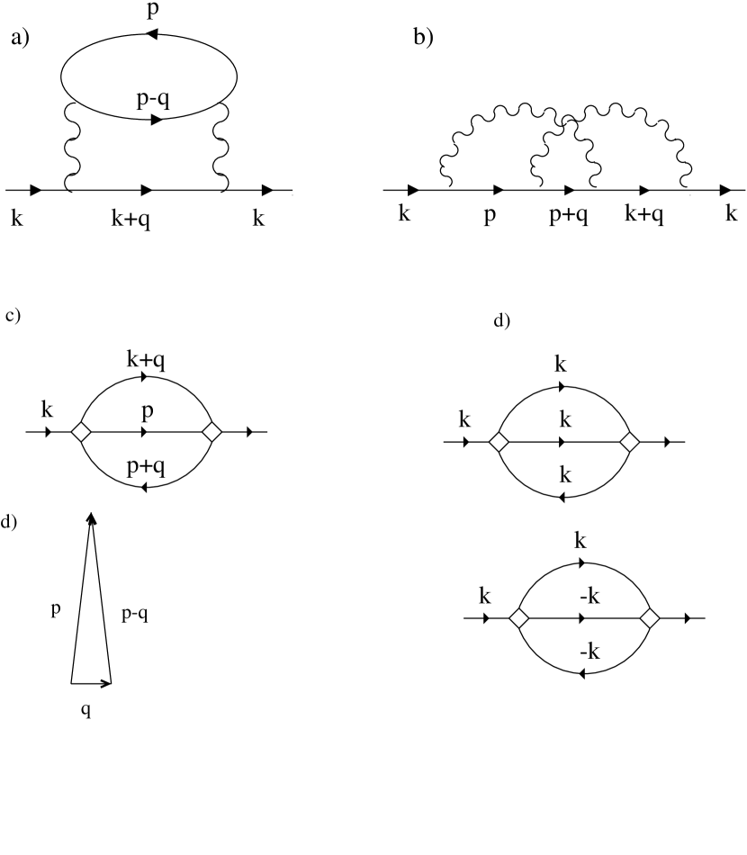
Fig. 3.: a) and b) Non-trivial second order diagrams for the self-energy. c) Same diagrams as in a) and b) re-drawn as a single “sunrise" diagram. d) Diagrams relevant for non-analytic terms in the self-energy. e) Kinematics of scattering in a polarization bubble: the dynamic part $\Pi\propto\omega/v_{F}q$ comes from the processes in which the internal fermionic momentum (${\vec{p}}$) is almost perpendicular to the external bosonic one (${\vec{q}}$).

In the perturbation theory, the Green’s function in (2.5) is a free one. Assuming the free-electron spectrum $\xi_{k}=(k^{2}-k_{F}^{2})/2m$,

$$\mathrm{Im}G^{R}\left(\varepsilon-\omega,\vec{k}-\vec{q}\right)=-\pi\delta\left(\varepsilon-\omega-\xi_{k}+\vec{v}_{k}\cdot\vec{q}-q^{2}/2m\right).$$

On the mass shell,

$$\mathrm{Im}G^{R}\left(\varepsilon-\omega,\vec{k}-\vec{q}\right)|_{\varepsilon=\xi_{k}}=-\pi\delta\left(\omega-\vec{v}_{k}\cdot\vec{q}+q^{2}/2m\right).$$

The argument of the delta-function simply expresses the energy and momentum conservation for a process $\varepsilon\rightarrow\varepsilon-\omega,\vec{k}\rightarrow\vec{k}-\vec{q}.$ The angular integral involves only the delta-function. For any $D,$ this integral gives

$$\langle\delta\left(\dots\right)\rangle_{\Omega}=\frac{1}{v_{F}q}A_{D}\left(\frac{\omega+q^{2}/2m}{v_{F}q}\right),$$

where $v_{k}$ was replaced by $v_{F}$ because all the action takes place near the Fermi surface. For $D=3$ and $D=2$,

$$A_{3}\left(x\right) = 2\theta(1-|x|);$$

$$A_{2}\left(x\right) = \frac{2\theta\left(1-\left|x\right|\right)}{\sqrt{1-x^{2}}}.$$

The constraint on the argument of $A_{D}$ is purely geometric: the magnitude of the cosine of the angle between $\vec{k}$ and $\vec{q}$ has to be less then one. For power-counting purposes, function $A_{D}$ has a dimensionality of 1. Therefore, its only role is to provide a lower cut-off for the momentum integral. Then, by power counting

$$\mathrm{Im}\Sigma^{R}\left(\varepsilon\right)\sim\frac{1}{v_{F}Q^{D}}\int_{0}^{\varepsilon}d\omega\omega\int_{q\geq\left|\omega\right|/v_{F}}dqq^{D-2}U\left(\frac{\left|\omega\right|}{v_{F}q},\frac{q}{Q}\right).$$ (2.6)

Now, if the integral over $q$ is dominated by $q\sim Q$ and is convergent in the infrared, one can put $\omega=0$ in this integral. After this step, the integrals over $\omega$ and $q$ decouple. The $\omega-$ integral gives $\varepsilon^{2}$ regardless of the nature of the interaction and dimensionality whereas the $q-$ integral supplies a prefactor which entails all the details of the interaction

$$\mathrm{Im}\Sigma^{R}\left(\varepsilon\right)=C_{D}\frac{\varepsilon^{2}}{v_{F}Q}.$$

For example, for a screened Coulomb interaction in the weak-coupling (high-density) limit $Q=\kappa$, where $\kappa$ is the screening wavevector, we have in 3D

$$-\mathrm{Im}\Sigma^{R}\left(\varepsilon\right)=\frac{\pi^{2}}{64}\frac{\kappa}{k_{F}}\frac{\varepsilon^{2}}{E_{F}}.$$

Now we can formulate a sufficient (but not necessary) condition for the Fermi-liquid behavior. It will occur whenever if kinematics of scattering is such that the typical momentum transfers are determined by some internal and, what is crucial, $\omega-$ independent scale, whereas the energy transfers are of order of the quasi-particle energy (or temperature). Excluding special situations, such as the high-density limit of the Coulomb interaction, $Q$ is generically of order of the ultraviolet range of the problem $\sim k_{F}.$ In other words, isotropic scattering guarantees a $\varepsilon^{2}$- behavior. Small-angle scattering with typical angles of order $\varepsilon/v_{F}\ll Q\ll k_{F}$ gives this behavior as well.

The $\varepsilon^{2}-$ result seems to be quite general under the assumptions made. When and why these assumptions are violated?

A long-range interaction, associated with small-angle scattering, is known to destroy the FL. For example, transverse long-range (current-current [44] or gauge [45]) interactions, which–unlike the Coulomb one–are not screened by electrons, lead to the breakdown of the Fermi liquid. However, the current-current interaction is of the relativistic origin and hence does the trick only at relativistically small energy scales, whereas the gauge interaction occurs only under special circumstances, such as near half-filling or for composite fermions. What about a generic case when nothing of this kind happens? It turns out that even if the bare interaction is of the most benign form, e.g., a delta-function in real space, there are deviations from a (perceived) FL behavior. These deviations get amplified as the system dimensionality is lowered, and, eventually, lead to a complete breakdown of the FL in 1D.

A formal reason for the deviation from the FL-behavior is that the argument which led us to the $\varepsilon^{2}$-term is good only in the leading order in $\omega/qv_{F}.$ Recall that the angular integration gives us $q^{-1}$ factors in all dimensions, and, to arrive at the $\varepsilon^{2}$ result we put $\omega=0$ in functions $A_{D}$ and $U.$ If we want to get a next term in $\varepsilon,$ then we need to expand $U$ and $A$ in $\omega.$ Had such expansions generated regular series, Im$\Sigma^{R}$ would have also formed regular series in $\varepsilon^{2}$: Im$\Sigma^{R}=a\varepsilon^{2}+b\varepsilon^{4}+c\varepsilon^{6}+\dots.$ However, each factor of $\omega$ comes with $q^{-1}$, so that no matter how high the dimensionality is, at some order of $\omega/v_{F}q$ we are bound to have an infrared divergence.

2.1 Long-range effective interaction

Let’s look at the simplest case of a point-like interaction. A frequency dependence of the self-energy arises already at the second order. At this order, two diagrams in Fig. 3 are of interest to us. For a contact interaction, diagram b) is just -1/2 of a) (which can be seen by integrating over the fermionic momentum $\vec{p}$ first), so we will lump them together. Two given fermions interact via polarizing the medium consisting of other fermions. Hence, the effective interaction at the second order is just proportional to the polarization bubble

$$\mathrm{Im}V^{R}(\omega,q)=-U^{2}\mathrm{Im}\Pi^{R}(\omega,q).$$

Let’s focus on small angle-scattering first: $q\ll 2k_{F}$. It turns out that in all three dimensions, the bubble has a similar form (see Appendix Appendix A for an explicit derivation of this result)

$$-\mathrm{Im}\Pi^{R}(\omega,q)=\nu_{D}\frac{\omega}{v_{F}q}B_{D}\left(\frac{\omega}{v_{F}q}\right),$$ (2.7)

where $\nu_{D}=a_{D}mk_{F}^{D-2}$ is the DoS in $D$ dimensions [$a_{3}=(2\pi)^{-2},$ $a_{2}=(2\pi)^{-1},$ $a_{1}=1/2\pi$] and $B_{D}$ is a dimensionless function, whose main role is to impose a constraint $\omega\leq v_{F}q$ in 2D and 3D and $\omega=v_{F}q$ in 1D.  Eq. (2.7) entails the physics of Landau damping. The constraint arises because collective excitations–charge- and spin-density waves– decay into particle-hole pairs. Decay occurs only if bosonic momentum and frequency ($q$ and $\omega$) are within the particle-hole continuum (cf. Fig. 4).

Fig. 4.: Particle-hole continua for $D>1$ (left) and $D=1$ (right). For the 1D case, only half of the continuum ($q>0$) is shown.

For $D>1,$ the boundary of the continuum for small $\omega$ and $q$ is $\omega=v_{F}q$, hence the decay takes place if $\omega<v_{F}q.$ The rest of Eq. (2.7) can be understood by dimensional analysis. Indeed, $\Pi^{R}$ is the retarded density-density correlation function; hence, by the same argument we applied to Im$V^{R},$ its imaginary part must be odd in $\omega.$ For $q\ll k_{F},$ the only combination of units of frequency is $v_{F}q,$ and the frequency enters as $\omega/v_{F}q.$ Finally, a factor $\nu_{D}$ makes the overall units right. In 1D, the difference is that the continuum shrinks to a single line $\omega=v_{F}q,$ hence decay of collective excitations is possible only on this line. In 3D, function $B_{3}$ is simply a $\theta-$ function

$$\mathrm{Im}\Pi^{R}(\omega,q)=-\nu_{3}\frac{\omega}{v_{F}q}\theta\left(q-\left|\omega/v_{F}\right|\right).$$

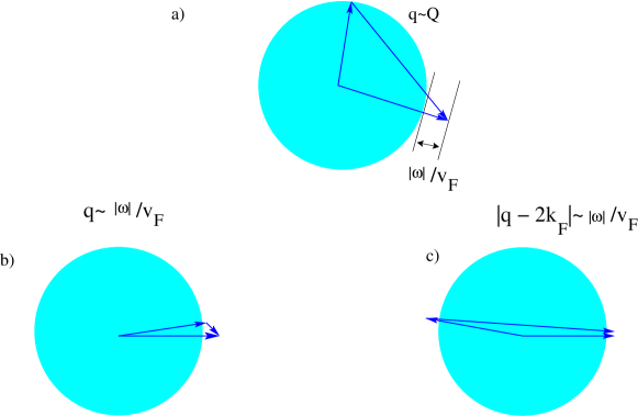
Fig. 5.: Kinematics of scattering. a) “Any-angle” scattering. Momentum transfer $q$ is of order of the intrinsic scale of the interaction or $k_{F}$, whichever is smaller, and is independent of the energy transfer, $\omega$, which is of order of the initial energy $\epsilon$. This process contributes regular terms to the self-energy. b) Dynamic forward scattering: $q\sim|\omega|/v_{F}$. c) Dynamic backscattering: $|q-2k_{F}|\sim|\omega|/v_{F}$. Processes b) and c) are responsible for the non-analytic terms in the self-energy.

Next-to-leading term in the expansion of Im$\Sigma^{R}$ in $\varepsilon$ comes from retaining the lower limit in the momentum integral of Eq. (2.6), upon which we get

$$-\mathrm{Im}\Sigma^{R} \sim U^{2}mk_{F}\int_{0}^{\varepsilon}d\omega\int_{\omega/v_{F}}^{Q\sim k_{F}}dqq^{2}\frac{1}{v_{F}q}\frac{\omega}{v_{F}q}$$

$$\sim U^{2}\frac{mk_{F}}{v_{F}^{2}}\int_{0}^{\varepsilon}d\omega\omega\left[\underbrace{k_{F}}_{\text{FL }}-\underbrace{\frac{\omega}{v_{F}}}_{\text{beyond FL}}\right]$$

$$\sim a\varepsilon^{2}-b\left|\varepsilon\right|^{3}.$$

The first term in the square brackets is the FL contribution that comes from $q\sim Q.$ The second term is a correction to the FL coming from $q\sim\omega/v_{F}.$ Thus, contrary to a naive expectation an expansion in $\varepsilon$ is non-analytic. The fraction of phase space for small-angle scattering is small–most of the self-energy comes from large-angle scattering events ($q\sim Q$); but we already start to see the importance of the small-angle processes. Applying Kramers-Kronig transformation to the non-analytic part ($\left|\varepsilon\right|^{3})$ in Im$\Sigma^{R},$ we get a corresponding non-analytic contribution to the real part as

$$\left(\mathrm{Re}\Sigma^{R}\right)_{\mathrm{non-an}}\propto\varepsilon^{3}\ln\left|\varepsilon\right|.$$

Correspondingly, specific heat which, by power counting, is obtained from Re$\Sigma^{R}$ by replacing each $\varepsilon$ by $T$, also acquires a non-analytic term

$$C(T)=\gamma_{3}T+\beta_{3}T^{3}\ln T.$$

This is the familiar $T^{3}\ln T$ term, observed both in He³ [40] and metals [41] (mostly, heavy-fermion materials) .

In 2D, the situation is more dramatic. The $q-$ integral diverges now logarithmically in the infrared:

$$-\mathrm{Im}\Sigma^{R}\left(\omega\right) \sim \frac{U^{2}}{v_{F}^{2}}m\int_{0}^{\varepsilon}d\omega\omega\int_{\sim\left|\omega\right|/v_{F}}^{\sim k_{F}}\frac{dq}{q}$$

$$\sim \frac{U^{2}}{v_{F}}m\varepsilon^{2}\ln\frac{E_{F}}{\left|\varepsilon\right|}.$$

Now, dynamic forward-scattering (with transfers $q\sim\omega/v_{F})$ is not a perturbation anymore: on the contrary, the $\varepsilon$ dependence of Im$\Sigma^{R}$ is dominated by forward scattering (the $\varepsilon^{2}\ln\left|\varepsilon\right|$-term is larger than the “any-angle” $\varepsilon^{2}$-contribution ). Correspondingly, the real part acquires a non-analytic term Re$\Sigma\propto\varepsilon\left|\varepsilon\right|$, and the specific heat behaves as

$$C(T)=\gamma_{2}T-\beta_{2}T^{2}.$$

The non-analytic $T^{2}$-term in the specific heat has been observed in recent experiments on monolayers of He³ adsorbed on a solid substrate [43].

Finally, in 1D the same power-counting argument leads to Im$\Sigma^{R}\propto\left|\varepsilon\right|$ and Re$\Sigma^{R}\propto$ $\varepsilon\ln\left|\varepsilon\right|$ Correspondingly, the “correction” to the specific heat behaves as $T\ln T$ and is larger than the leading, $T-$ term. This is the ultimate case of dynamic forward scattering, whose precursors we have already seen in higher dimensions .

Even if the bare interaction is point-like, the effective one contains a long-range part at finite frequencies. Indeed, the non-analytic parts of $\Sigma$ and $C(T)$ come from the region of small $q,$ and hence large distances. Already to the second order in $U$, the effective interaction $\tilde{U}=U^{2}\Pi(\omega,q)$ is proportional to the dynamic polarization bubble of the electron gas, $\Pi\left(\omega,q\right)$. In all dimensions, Im$\Pi^{R}$ is universal and singular in $q$ for $\left|\omega\right|/v_{F}\ll q\ll k_{F}$

$$\text{Im}\Pi^{R}\left(\omega,q\right)\sim\nu_{D}\frac{\omega}{v_{F}|q|}.$$

Although the effective interaction is indeed screened at $q\rightarrow 0$ –and this is why the FL survives even if the bare interaction has a long-range tail–it has a slowly decaying tail in the intermediate range of $q.$ In real space, $\tilde{U}(r)$ behaves as $\omega/r^{D-1}$ at distances $k_{F}^{-1}\ll r\ll v_{F}/|\omega|$.

Thus, we have the same singular behavior of the bubble in all dimensions, and the results for the self-energy differ only because the phase volume $q^{D}$ is more effective in suppressing the singularity in higher dimensions than in lower ones.

There is one more special interval of $q$: $q\approx 2k_{F}$ , i.e., Kohn anomaly. Usually, the Kohn anomaly is associated with the $2k_{F}$- non-analyticity of the static bubble, and its most familiar manifestation is the Friedel oscillation in electron density produced by a static impurity (discussed later on). Here, the static Kohn anomaly is of no interest for us as we are dealing with dynamic processes. However, the dynamic bubble is also singular near $2k_{F}$. For example, in 2D,

$$\mathrm{Im}\Pi^{R}\left(q\approx 2k_{F},\omega\right)\propto\frac{\omega}{\sqrt{k_{F}\left(2k_{F}-q\right)}}\theta\left(2k_{F}-q\right).$$

Because of the one-sided singularity in $\mathrm{Im}\Pi^{R}$ near $q=2k_{F}$, the effective interaction oscillates and falls off as a power of $r$. By power counting, if a static Friedel oscillation falls off as $\sin 2k_{F}r/r^{D}$, then the dynamic one behaves as

$$\tilde{U}\propto\frac{\omega\sin 2k_{F}r}{r^{(D-1)/2}}.$$

Dynamic Kohn anomaly results in the same kind of non-analyticity in the self-energy (and thermodynamics) as the forward scattering. The “dangerous” range of $q$ now is $\left|q-2k_{F}\right|\sim\omega/v_{F}$–“dynamic backscattering”. It is remarkable that the non-analytic term in the self-energy is sensitive only to strictly forward or backscattering events, whereas processes with intermediate momentum transfers contribute only to analytic part of the self-energy. To see this, we perform the analysis of kinematics in the next section.

2.2 1D kinematics in higher dimensions

The similarity between non-FL behavior in 1D and non-analytic features in higher dimensions occurs already at the level of kinematics. Namely, one can make a rather strong statement: the non-analytic terms in the self-energy in higher dimensions result from essentially 1D scattering processes. Let’s come back to self-energy diagram 3a. In general, integrations over fermionic momentum $\vec{p}$ and bosonic $\vec{q}$ are independent of each other: one can first integrate over ($\vec{p},\varepsilon),$ forming a bubble, and then integrate over ($\vec{q},\omega$). Generically, $\vec{p}$ spans the entire Fermi surface. However, the non-analytic features in $\Sigma$ come not from generic but very specific $\vec{p}$ which are close to either to $\vec{k}$ or to $-\vec{k}.$

Fig. 6.: Scattering processes responsible for divergent and/or non-analytic corrections to the self-energy in 2D. a) “Forward scattering”–an analog of the “$g_{4}$”-process in 1D. All four fermionic momenta are close to each other. b) Backscattering–an analog of the “$g_{2}$”-process in 1D. The net momentum before and after collision is small. Initial momenta are close to final ones. Although the momentum transfer in such a process is small, we still refer to this process as “backscattering” (see the discussion in the main text). c) $2k_{F}-$ scattering.

Let’s focus on the 2D case. The $\varepsilon^{2}\ln|\varepsilon|$ term results from the product of two $q^{-1}$ -singularities: one is from the angular average of Im$G$ and the other one from the dynamic, $\omega/v_{F}q$, part of the bubble. In Appendix Appendix A, it is shown that the $\omega/v_{F}q$ singularity in the bubble comes from the region where $\vec{p}$ is almost perpendicular to $\vec{q}.$ Similarly, the angular averaging of Im$G$ also pins the angle between $\vec{k}$ and $\vec{q}$ to almost $90^{\circ}.$

$$\mathrm{Im}G^{R}(\varepsilon-\omega,\vec{k}-\vec{q}) = -\pi\delta\left(\varepsilon-\omega-qv_{F}\cos\theta^{\prime}\right)\rightarrow$$

$$\cos\theta^{\prime} = \frac{\varepsilon-\omega}{v_{F}q}\sim\frac{\omega}{v_{F}q}\ll 1\rightarrow\theta^{\prime}\approx\pi/2.$$

As $\vec{p}$ and $\vec{k}$ are almost perpendicular to the same vector ($\vec{q}$), they are either almost parallel or anti-parallel to each other. In terms of a symmetrized (“sunrise”) self-energy (cf. Fig. 3), it means that either all three internal momenta are parallel to the external one or one of the internal one is parallel to the external whereas the other two are anti-parallel . Thus we have three almost 1D processes:

• all four momenta (two initial and two final) are almost parallel to each other;

• the total momentum of the fermionic pair is near zero, whereas the transferred momentum is small;

• he total momentum of the fermionic pair is near zero, whereas the transferred momentum is near $2k_{F}$.

These are precisely the same 1D processes we are going to deal with in the next Section–the only difference is that in 2D, trajectories do have some angular spread, which is of order $\left|\omega\right|/E_{F}.$ The first one is known as “$g_{4}"$ (meaning: all four momenta are in the same direction) and the other one as “$g_{2}"$ (meaning: two out of four momenta are in the same direction). Both of these processes are of the forward-scattering type as the transferred momentum is small. In 1D, these processes correspond to scattering of fermions of same ($g_{4}$) or opposite chirality ($g_{2}$). The last ($2k_{F}$) process is known “$g_{1}"$ in 1D.

It turns out that of these two processes, the $g_{2}$- and $2k_{F}$- ones, are directly responsible for the $\varepsilon^{2}\ln\varepsilon$ behavior. The $g_{4}$-process leads to a mass-shell singularity in the self-energy both in 1D and 2D, discussed in the next section, but does not affect the thermodynamics, so we will leave it for now.

What about $2k_{F}-$ scattering? Suppose electron $\vec{k}$ scatters into $-\vec{k}$ emitting an electron-hole pair of momentum $2\vec{k}.$ In general, $2\vec{k}$ of the e-h pair may consist of any two fermionic momenta which differ by $2\vec{k}:$ $\vec{p}$ and $\vec{p}+2\vec{k}.$ But since $\left|2\vec{k}\right|\approx 2k_{F},$ the components of the e-h pair will be on the Fermi surface only if $\vec{p}\approx-\vec{k}$ and $\vec{p}+2\vec{k}\approx\vec{k}.$ Only in this case does the effective interaction (bubble) have a non-analytic form at finite frequency. Thus $2k_{F}$- scattering is also of the 1D nature for $D>1.$

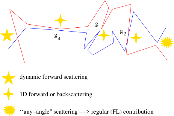
Fig. 7.: Typical trajectories of two interacting fermions. Explosion: “any-angle” scattering at a third fermion (not shown) which leads to a regular (FL) contribution. Five-corner star: dynamic forward scattering $q\sim|\omega|/v_{F}$. This process contributes to non-analyticity in 3D (to third order in the interaction) but not in 2D. Four-corner star: 1D dynamic forward and backscattering events, contributing to non-analyticities both in 3D and 2D.

What we have said above, can be summarized in the following pictorial way. Suppose we follow the trajectories of two fermions, as shown in Fig. 7. There are several types of scattering processes. First, there is “any-angle” scattering which, in our particular example, occurs at a third fermion whose trajectory is not shown. This scattering contributes regular, FL terms both to the self-energy and thermodynamics. Second, there are dynamic forward-scattering events, when $q\sim\left|\omega\right|/v_{F}.$ These are not 1D processes, as fermionic trajectories enter the interaction region at an arbitrary angle to each other. In 3D, a third order in such processes results in the non-analytic behavior of $C(T)$–this is the origin of the “paramagnon” anomaly in $C(T).$ In 2D, dynamic forward scattering does not lead to non-analyticity. Finally, there are processes, marked by“$g_{1}$”, “$g_{2}$”, and “$g_{4}$", when electrons conspire to align their initial momenta so that they are either parallel or antiparallel to each other. These processes determine the non-analytic parts of $\Sigma$ and thermodynamics in 2D (and also, formally, for $D<2.$) A crossover between $D>1$ and $D=1$ occurs when all other processes but $g_{1},$ $g_{2},$ and $g_{4}$ are eliminated by a geometrical constraint.

We see that for non-analytic terms in the self-energy (and thermodynamics), large-angle scattering does not matter. Everything is determined by essentially 1D processes. As a result, if the bare interaction has some $q$ dependence, only two Fourier components matter: $U(0)$ and $U(2k_{F}).$ For example, in 2D

$$\text{Im}\Sigma^{R}\left(\varepsilon\right) \propto \left[U^{2}\left(0\right)+U^{2}\left(2k_{F}\right)-U(0)U(2k_{F})\right]\varepsilon^{2}\ln\left|\varepsilon\right|;$$

$$\text{Re}\Sigma^{R}\left(\omega\right) \propto \left[U^{2}\left(0\right)+U^{2}\left(2k_{F}\right)-U(0)U(2k_{F})\right]\varepsilon\left|\varepsilon\right|;$$

$$C(T)/T = \gamma^{\ast}-a\left[U^{2}\left(0\right)+U^{2}\left(2k_{F}\right)-U(0)U(2k_{F})\right]T;$$

$$\chi_{s}(Q,T) = \chi_{s}^{\ast}\left(0\right)+bU^{2}\left(2k_{F}\right)\max\left\{v_{F}Q,T\right\};$$

where $a$ and $b$ are coefficients. These perturbative results can be generalized for the Fermi-liquid case, when the interaction is not necessarily weak. Then the leading, analytic parts of $C(T)$ and $\chi_{s}$ are determined by the angular harmonics of the Landau interaction function

$$\hat{F}\left(\vec{p},\vec{p}^{\prime}\right)=F_{s}\left(\theta\right)\hat{I}+F_{a}\left(\theta\right)\vec{\sigma}\cdot\vec{\sigma}^{\prime},$$

where $\theta$ is the angle between $\vec{p}$ and $\vec{p}^{\prime}.$ In particular,

$$\gamma^{\ast} = \gamma_{0}\left(1+\langle\cos\theta F_{s}\rangle\right);$$

$$\chi_{s}^{\ast}\left(0\right) = \chi_{s}^{0}\frac{1+\langle\cos\theta F_{s}\rangle}{1+\langle F_{a}\rangle},$$

where $\gamma_{0}$ and $\chi_{s}^{0}$ are the corresponding quantities for the Fermi gas. Because of the angular averaging, the FL part is rather insensitive to the details of the interaction. As generically $F_{s}$ and $F_{a}$ are regular functions of $\theta,$ the whole Fermi surface contributes to the FL renormalizations. Vertices $U(0)$ and $U(2k_{F})$, occurring in the perturbative expressions, are replaced by scattering amplitudes at angle $\theta=\pi$

$$\hat{A}\left(\vec{p},\vec{p}^{\prime}\right)=A_{s}\left(\theta\right)\hat{I}+A_{a}\left(\theta\right)\vec{\sigma}\cdot\vec{\sigma}^{\prime},$$

Beyond the perturbation theory [37],

$$C(T)/T = \gamma^{\ast}-\bar{a}\left[A_{s}^{2}\left(\pi\right)+3A_{a}^{2}\left(\pi\right)\right]T;$$

$$\chi_{s}(Q,T) = \chi_{s}^{\ast}\left(0\right)+\bar{b}A_{a}^{2}\left(\pi\right)\max\left\{v_{F}Q,T\right\}.$$

Non-analytic parts are not subject to angular averaging and are sensitive to a detailed behavior of $A_{s,a}$ near $\theta=\pi$.

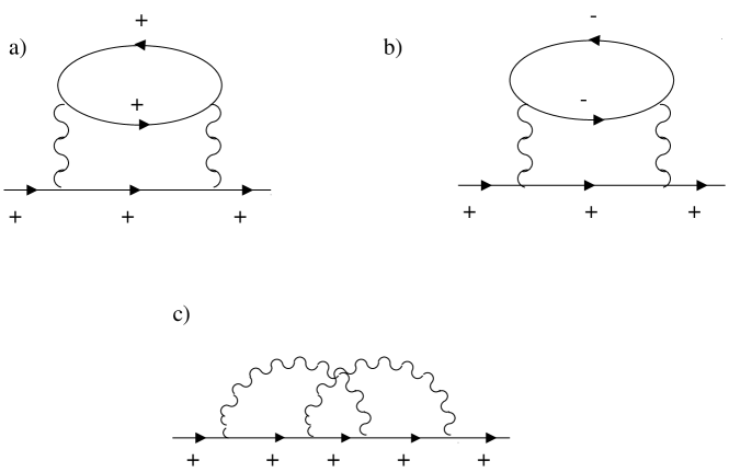
Fig. 8.: Self-energy in 1D. $\pm$ refer to right (left)-moving fermions.

2.3 Infrared catastrophe

2.3.1 1D

By now, it is well-known that the FL breaks down in 1D and an attempt to apply the perturbation theory to 1D problem results in singularities. Let’s see what precisely goes wrong in 1D. I begin with considering the interaction of fermions of opposite chirality, as in diagram Fig. 8b. Physically, a right-moving fermion emits (and then re-absorbs) left-moving quanta of density excitations (same for left-moving fermion emitting/absorbing right-moving quanta). Now, instead of the order-of-magnitude estimate (2.7), which is good in all dimensions but only for power-counting purposes, I am going to use an exact expression for the bubble, Eq. (B. 4), formed by left-moving fermions. On the Fermi surface ($k=k_{F}$, we have

$$-\mathrm{Im}\Sigma_{+-}^{R}\left(\varepsilon\right) \sim U^{2}\nu_{1}\int_{0}^{\varepsilon}d\omega\int dq\mathrm{Im}G_{+}^{R}\left(\varepsilon-\omega,k-q\right)\text{Im}\mathrm{\Pi}_{-}^{R}$$

$$\sim U^{2}\nu_{1}\int_{0}^{\varepsilon}d\omega\int dq\delta\left(\varepsilon-\omega+v_{F}q\right)\left(\omega/v_{F}\right)\delta\left(\omega+v_{F}q\right)$$

$$\sim g^{2}\left|\varepsilon\right|,$$

where $g\equiv U/v_{F}$ is the dimensionless coupling constant. The corresponding real part behaves as $\varepsilon\ln\left|\varepsilon\right|.$ What we got is bad, as $\mathrm{Im}\Sigma^{R}$ scales with $\varepsilon$ in the same way as the energy of a free excitation above the Fermi level and Re$\Sigma^{R}$ increases faster than $\varepsilon$ (which means that the effective mass depends on $\varepsilon$ as $\ln|\varepsilon|)$, but not too bad because, as long as $g\ll 1$, the breakdown of the quasi-particle picture occurs only at exponentially small energy scales: $\varepsilon\lesssim E_{F}\exp(-1/g^{2}).$ Now, let’s look at scattering of fermions of the same chirality. This time, I choose to be away from the mass shell.

$$-\mathrm{Im}\Sigma_{++}^{R} \propto \int_{0}^{\varepsilon}d\omega\int dq\underbrace{\delta\left(\varepsilon-\omega-v_{F}\left(k-q\right)\right)}_{\mathrm{Im}G_{+}^{R}}\underbrace{\omega\delta\left(\omega-v_{F}q\right)}_{\mathrm{Im}\Pi_{+}^{R}}$$ (2.8)

$$= \varepsilon^{2}\delta\left(\varepsilon-v_{F}k\right).$$ (2.9)

It is not difficult to see that the full (complex) self-energy is simply

$$\Sigma_{++}^{R}\propto-\frac{\varepsilon^{2}}{\varepsilon-v_{F}k+i0^{+}}.$$ (2.10)

On the mass shell ($\varepsilon=v_{F}k)$ we have a strong–delta-function–singularity. This anomaly was discovered by Bychkov, Gor’kov, and Dzyaloshinskii back in the 60s [52], who called it the “infrared catastrophe”. Indeed, it is similar to an infrared catastrophe in QED, where an electron can emit an infinite number of soft photons. Likewise, since we have linearized the spectrum, a 1D fermion can emit an infinite number of soft bosons: quanta of charge- and spin-density excitations. The point is that in 1D there is a perfect match between momentum and energy conservations for a process of emission (or absorption) of a boson with energy and momentum related by $\omega=v_{F}q:$

$$k^{\prime} = k-q$$

$$\varepsilon^{\prime} = \varepsilon-\omega=v_{F}k-v_{F}q=v_{F}\left(k-q\right).$$

On the mass-shell, the energy and momentum conservations are equivalent. Imagine that you want to find a probability of certain scattering process using a Fermi Golden rule. Then you have a product of two $\delta-$ functions: one reflecting the momentum and other energy conservation. But if the arguments of the delta-functions are the same, you have an essential singularity: a square of the delta-function. As a result, the corresponding probability diverges.

A pole in the self-energy [Eq. (2.10)] indicates the non-perturbative and specifically 1D effect: spin-charge separation. Indeed, substituting Eq. (2.10) we get two poles corresponding to excitations propagating with velocities $v_{F}\left(1\pm g\right)$ (recall that $g\ll 1).$ This peculiar feature is confirmed by an exact solution (see Section 3): already the $g_{4}-$interaction leads to a spin-charge separation (but not to anomalous scaling). What we did not get quite right is that the velocities of both–spin- and charge-modes–are modified by the interactions. In fact,the exact solution shows that the velocity of the spin-mode remains equal to $v_{F},$ whereas the velocity of the charge mode is modified.

Obviously, there is no spin-charge separation for spinless electrons. Indeed, in this case diagram Fig. 8a does not have an additional factor of two as compared to Fig. 8c (but is still of opposite sign), so that the forward-scattering parts of these two diagrams cancel each other. As a result, there is no infrared catastrophe for spinless fermions.

2.3.2 2D

What we considered in the previous section sounds like an essentially 1D effect. However, a similar effect exists also in 2D (more generally, for $1\leq D\leq 2$). This emphasizes once again that the difference between $D=1$ and $D>1$ is not as dramatic as it seems.

In 2D, the self-energy also diverges on the mass shell, if one linearizes the electron’s spectrum, albeit the divergence is weaker than in 1D–to second order, it is logarithmic . The origin of the divergence can be traced back to the form of the polarization bubble at small momentum transfer, Eq. (A. 1). Integrating over the angle in 2D, we get

$$\text{Im}\Pi^{R}(\omega,q)=-\left(\frac{m}{2\pi}\right)\frac{\omega}{\sqrt{\left(v_{F}q\right)^{2}-\omega^{2}}}\theta\left(v_{F}q-\left|\omega\right|\right).$$ (2.11)

$\text{Im}\Pi^{R}(\omega,q)$ has a square-root singularity at the boundary of the particle-hole continuum, i.e., at $\omega=v_{F}q$. (This is a threshold singularity of the van Hove type: the band of soft electron-hole pairs is terminated at $\omega=v_{F}q,$ but the spectral weight of the pairs is peaked at the band edge). On the other hand, expanding $\epsilon_{\mathbf{k}+\mathbf{q}}$ in $G^{R}(\varepsilon+\omega,\mathbf{k}+$$q$$)$ as $\xi_{\mathbf{k+q}}=\xi_{k}+v_{F}q\cos\theta$ and integrating over $\theta$, we obtain another square-root singularity

$$\int d\theta\text{Im}G^{R}=-2\pi\left[\left(v_{F}q\right)^{2}-\left(\varepsilon+\omega-\xi_{k}\right)^{2}\right]^{-1/2}.$$ (2.12)

On the mass shell ($\omega=\xi_{k}$), the arguments of the square roots in Eqs. (2.11) and (2.12) coincide, and the integral over $q$ diverges logarithmically. The resulting contribution to Im$\Sigma^{R}$ diverges on the mass shell ($\varepsilon=\xi_{k})$ [53, 54, 55],[34],[37]

$$\text{Im}\Sigma_{g_{4}}^{R}\left(\varepsilon,k\right)=-\frac{u^{2}}{8\pi}\frac{\varepsilon^{2}}{E_{F}}\ln\frac{E_{F}}{|\varepsilon-\xi_{k}|},$$

where $\Delta\equiv\varepsilon-\xi_{k}$ and $u\equiv mU/2\pi.$ The process responsible for the log-singularity is the “$g_{4}"$ process in Fig. 6. On the other hand, $g_{2}$ and $g_{1}$ processes give a contribution which is finite on the mass shell

$$\text{Im}\Sigma_{g_{1}+g_{2}}^{R}\left(\varepsilon,k\right)=-\frac{u^{2}}{4\pi}\frac{\varepsilon^{2}}{E_{F}}\ln\frac{E_{F}}{|\varepsilon+\xi_{k}|}.$$

(The divergence at $\varepsilon=-\xi_{k}$ is spurious and is removed by going beyond the log-accuracy [34],[37].) We see therefore that the familiar form of the self-energy in 2D [$\varepsilon^{2}\ln\left|\varepsilon\right|$, see Ref. [56]] is valid only on the Fermi surface $\left(\xi_{k}=0\right).$ The logarithmic singularity in Im$\Sigma^{R}$ on the mass shell is eliminated by retaining the finite curvature of single-particle spectrum (which amounts to keeping the $q^{2}/2m$ term in $\xi_{\vec{k}+\vec{q}}).$ This brings in a new scale $\varepsilon^{2}/E_{F}$. The emerging singularity in (2.3.2) is regularized at $\left|\varepsilon-\xi_{k}\right|\sim\varepsilon^{2}/E_{F}$ and the $\varepsilon^{2}\ln\left|\varepsilon\right|$ behavior is restored. However, higher orders diverge as power-laws and finite curvature does not help to regularize them. This means that–in contrast to 3D–the perturbation theory must be re-summed even for an infinitesimally weak interaction. Once this is done, the singularities are removed. Re-summation also helps to understand the reason for the problems in the perturbation theory. In fact, what we were trying to do was to take into account a non-perturbative effect–an interaction with the zero-sound mode–via a perturbation theory. Once all orders are re-summed, the zero-sound mode splits off the continuum boundary–now it is a propagating mode with velocity $c>v_{F}.$ This splitting is what regularizes the divergences. The resulting state is essentially a FL: the leading term in $\Sigma$ behaves as $\varepsilon^{2}\ln\left|\varepsilon\right|.$ However, some non-perturbative features remain: for example, the spectral function exhibits a second peak away from the mass shell corresponding to the emission of the zero-sound waves by fermions. A two-peak structure of the spectral function is reminiscent of the spin-charge separation, although we do not really have a spin-charge separation here: in contrast to the 1D case, the spin-density collective mode lies within the continuum and is damped by the particle-hole pairs.

3 Dzyaloshinskii-Larkin solution of the Tomonaga-Luttinger model

3.1 Hamiltonian, anomalous commutators, and conservation laws

In the Tomonaga-Luttinger model [57],[58] one considers a system of 1D spin-1/2 fermions with a linearized dispersion. Only forward scattering of left- and right-moving fermions is taken into account ($g_{2}$ and $g_{4}-$ processes), whereas backscattering is neglected. This last assumption means that the interaction potential is of sufficiently long-range, so that $U\left(2k_{F}\right)\ll U\left(0\right).$ [We will come back to this condition later.] Coupling between fermions of the same chirality ($g_{4}$) is assumed to be different from coupling between fermions of different chirality ($g_{2}).$ If the original Hamiltonian contains only density-density interaction, then $g_{2}=g_{4}.$ A difference between $g_{2}$ and $g_{4}$ leads to an unphysical (within this model) current-current interaction. We will keep $g_{2}\neq g_{4}$, however, at the intermediate steps of the calculations as it helps to elucidate certain points. At the end, one can make $g_{2}$ equal to $g_{4}$ without any penalty. In addition, in some physical situations, $g_{2}\neq g_{4}$ . In what follows I will follow the original paper by Dzyaloshinskii and Larkin (DL) [59] and a paper by Metzner and di Castro [60], where the Ward identity used by Dzyaloshinskii and Larkin is derived in a detailed way.

The Hamiltonian of the model is written as

$$H = H_{0}+H_{\mathrm{int}};$$

$$H_{\mathrm{int}} \equiv H_{2}+H_{4},$$

where

$$H_{0}=v_{F}\sum_{k,\sigma}k\left(a_{+,\sigma}^{\dagger}(k)a_{+,\sigma}(k)-a_{-,\sigma}^{\dagger}(k)a_{-,\sigma}(k)\right)$$

is the Hamiltonian of free fermions ($\pm$ denote right/left moving fermions and $\sigma$ is the spin projection) and

$$H_{2} = \frac{g_{2}}{L}\sum_{q}\sum_{\sigma,\sigma^{\prime}}\rho_{+,\sigma}\left(q\right)\rho_{-,\sigma^{\prime}}\left(-q\right);$$

$$H_{4} = \frac{g_{4}}{2L}\sum_{q}\sum_{\sigma,\sigma^{\prime}}\rho_{+,\sigma}\left(q\right)\rho_{+,\sigma^{\prime}}\left(-q\right)+\rho_{-,\sigma}\left(q\right)\rho_{-,\sigma^{\prime}}\left(-q\right),$$

with

$$\rho_{\pm,\sigma}=\sum_{k}a_{\pm,\sigma}^{\dagger}\left(k+q\right)a_{\pm,\sigma}\left(k\right).$$

To avoid additional complications, I assume that the interaction is spin-independent. To simplify the notations and to emphasize the similarity between this model and QED, I will set $v_{F}$ to unity in this section.

Introducing the chiral charge- and spin densities as

$$\rho_{\pm}^{c} = \rho_{\pm,\uparrow}+\rho_{\pm,\downarrow};$$

$$\rho_{\pm}^{s} = \rho_{\pm,\uparrow}-\rho_{\pm,\downarrow},$$

and total charge density and current as

$$\rho^{c} = \rho_{+}^{c}+\rho_{-}^{c};$$

$$j^{c} = \rho_{+}^{c}-\rho_{-}^{c},$$

the interaction part of the Hamiltonian reduces to

$$H_{\mathrm{int}}=\sum_{q}\frac{1}{2}\left(g_{2}+g_{4}\right)\rho^{c}\left(q\right)\rho^{c}\left(-q\right)+\frac{1}{2}\left(g_{4}-g_{2}\right)j^{c}\left(q\right)j^{c}\left(-q\right).$$ (3.1)

As we have already said, for $g_{2}=g_{4},$ the interaction is of a pure density-density type. Notice also that the spin density and current drop out of the Hamiltonian–this is to be expected for a spin-invariant interaction. To make a link with QED, let us introduce Minkowski current $j^{\mu}$ with $\mu=0,1$ so that $j^{0}=\rho^{c}$ (=$j_{0})$ and $j^{1}=j^{c}$ (=-$j_{1}).$ Then the interaction can be written as a 4-product of Minkowski currents in a Lorentz-invariant form

$$H_{\mathrm{int}}=\sum_{q}g_{\mu\nu}j_{\nu}j^{\nu},$$

where

$$g_{00} = \frac{1}{2}\left(g_{2}+g_{4}\right);$$

$$g_{11} = \frac{1}{2}\left(g_{4}-g_{2}\right);$$

$$g_{01} = g_{10}=0.$$ (3.2)

In what follows, we will need the following anomalous commutators

$$\left[\rho_{\pm,\sigma}\left(q\right),H_{0}\right] = \pm q\rho_{\pm,\sigma}\left(q\right);$$

$$\left[\rho_{\pm,\sigma}\left(q\right),H_{2}\right] = \pm\frac{g_{2}}{2\pi}q\rho_{\mp,\sigma}\left(q\right);$$

$$\left[\rho_{\pm,\sigma}\left(q\right),H_{4}\right] = \pm\frac{g_{4}}{2\pi}q\rho_{\pm,\sigma}\left(q\right).$$

The derivation of these commutation relations can be found in a number of standard sources [61, 10] and I will not present it here. Adding up the commutators, we get

$$\left[\rho_{\pm,\sigma},H\right] = \left[\rho_{\pm,\sigma},H_{0}+H_{2}+H_{4}\right]$$

$$= \pm q\rho_{\pm,\sigma}\pm\frac{g_{2}}{2\pi}q\rho_{\mp}^{c}\pm\frac{g_{4}}{2\pi}q\rho_{\pm}^{c}$$

Adding up equations for spin-up and -down fermions, we obtain

$$\left[\rho_{\pm,}^{c},H\right]=\pm q\rho_{\pm}^{c}\pm\frac{g_{2}}{\pi}q\rho_{\mp}^{c}\pm\frac{g_{4}}{\pi}q\rho_{\pm}^{c}.$$

Finally, adding up the $\pm$ components yields

$$i\partial_{t}\rho^{c}=\left[\rho^{c},H\right]=v_{c}qj^{c},$$ (3.3)

where

$$v_{c}\equiv 1+\frac{g_{4}-g_{2}}{\pi}$$

(recall that $v_{F}=1).$ Eq. (3.3) is a continuity equation reflecting charge conservation. As if we did not have enough new notations, here is another one

$$Q^{\mu}=\left(\omega,q\right)$$

and

$$\mathcal{Q}^{\mu}=\left(\omega,v_{c}q\right).$$

In these notations and after a Fourier transform, the continuity equation can be written as

$$\mathcal{Q}_{\mu}j^{\mu}=0.$$

The same relation for free particles reads

$$Q_{\mu}j^{\mu}=0.$$

3.2 Reducible and irreducible vertices

Fig. 9.: a) Three-leg correlator $K$. b) Vertex part $\Lambda$.

Now, construct a mixed (fermion-boson) correlator

$$K_{\pm,\sigma}^{\mu}\left(k,q|t,t_{1},t_{1}^{\prime}\right)=-\langle Tj^{\mu}\left(q,t\right)a_{\pm,\sigma}\left(k,t_{1}\right)a_{\pm,\sigma}^{\dagger}\left(k+q,t_{1}\right)\rangle,$$ (3.4)

where $\mu=0,1$ and

$$j^{0} = \rho_{+}^{c}+\rho_{-}^{c};$$

$$j^{1} = \rho_{+}^{c}-\rho_{-}^{c}.$$

$K^{\mu}$ is an analog of the three-leg vertex in QED , except that in QED the “boson” is the $\mu-$ the component of the photon field

$$\mathrm{QED:}\text{ }K^{\mu}=-\langle TA^{\mu}a\bar{a}\rangle.$$

A diagrammatic representation of $K^{\mu}$ is a three-particle (one boson and two fermions) diagram (cf. Fig. 9a).

The diagrams with self-energy insertions to solid lines simply renormalize the Green’s functions. Absorbing these renormalizations, we single out the vertex part, re-writing $K^{\mu}$ as

$$K^{\mu}=G^{2}\Lambda^{\mu}.$$ (3.5)

Fig. 10.: Relation between vertices $\Lambda$ and $\Gamma$.

Notice that there are as many vertex parts as there are bosonic degrees of freedom. In (3+1) QED, $\Lambda^{0}$ is a scalar vertex and $\Lambda^{\mu=1,2,3}$ are the components of the vector vertex. Diagrams representing $\Lambda^{\mu}$ are shown in Fig. 9b. These series can be re-arranged further by separating the photon-irreducible vertex part, $\Gamma^{\mu}$. A photon-irreducible part is obtained by separating the corrections to the bosonic line, i.e., taking into account polarization. Vertices $\Lambda^{\mu}$ and $\Gamma^{\mu}$ are related via a kind of Dyson equation, which is simpler than the usual Dyson in a sense that there is no $\Lambda^{\mu}$ on the right-hand-side. Diagrammatically, this relation is represented by Fig.10 where a shaded bubble is an exact (renormalized) current-current correlation function

$$A^{\mu\nu}\left(q,t\right)=-\frac{i}{V}\langle j^{\mu}\left(q,t\right)j^{\mu}\left(-q,0\right)\rangle.$$

Algebraically, equation in Fig.10 says

$$\Lambda_{\pm,\sigma}^{\mu}=\Gamma_{\pm,\sigma}^{\mu}+A^{\mu\nu}g_{\mu\lambda}\Gamma_{\pm,\sigma}^{\lambda}.$$ (3.6)

(We remind the reader that indices $\pm,\sigma$ simply specify the fermionic flavor which is not mixed in our approximation of forward-scattering and spin-independent forces, so all relations are applicable to each individual flavor). The coupling constants $g^{\mu\nu}$ relate currents to densities. According to Eqs. (3.1) and (3.2), densities couple to densities and currents to currents with no cross terms. Opening the matrix product in Eq. (3.6), we obtain

$$\Lambda_{i}^{\mu}=\Gamma_{i}^{\mu}+A^{\mu 0}g_{00}\Gamma^{0}+A^{\mu 1}g_{11}\Gamma^{1}.$$ (3.7)

3.3 Ward identities

A Ward identity for vertex $\Lambda^{\mu}$ is obtained by applying $i\partial_{t}$ to $K^{\mu}$ in Eq. (3.4) and using the continuity equation (3.4). Performing this operations and Fourier transforming in time, we obtain

$$\mathcal{Q}_{\mu}K_{i}^{\mu}\left(K,Q\right)=G_{i}\left(K\right)-G_{i}\left(K+Q\right),$$

where $i$ denotes the branch

$$i\equiv\pm,\sigma.$$

Recalling Eq. (3.5), we see that the Ward identity becomes

$$\mathcal{Q}_{\mu}\Lambda_{i}^{\mu}\left(K,Q\right)=G_{i}^{-1}\left(K+Q\right)-G_{i}^{-1}\left(K\right),$$ (3.8)

which is identical to a corresponding identity in QED. For those who like to see things not masked by fancy notations, here is Eq. (3.8) in an explicit form

$$\omega\Lambda_{i}^{0}\left(\varepsilon,k;\omega,q\right)-v_{c}q\Lambda_{i}^{1}\left(\varepsilon,k;\omega,q\right)=G_{i}^{-1}\left(\varepsilon+\omega,k+q\right)-G_{i}^{-1}\left(\varepsilon,k\right).$$ (3.9)

Notice that Eqs.(3.8,3.9) contain renormalized velocity $v_{c}.$ In what follows, we will actually need a Ward identity not for $\Lambda^{\mu}$ but for the photon-irreducible vertex $\Gamma^{\mu}.$ This one is obtained by deriving the continuity equation for 4-current correlation function $A^{\mu\nu}.$ To this end, one applies $i\partial_{t}$ to $A^{0\nu}$ and uses continuity equation (3.3), which yields

$$Q_{\mu}A^{\mu\nu}=\frac{2}{\pi}q\delta_{\nu,1}.$$ (3.11)

Now, we form a scalar product between $\mathcal{Q}_{\mu}$ and Eq. (3.7), using continuity equation for $A^{\mu\nu}$ (3.11). This brings us to

$$\mathcal{Q}_{\mu}\Lambda_{i}^{\mu}=Q_{\mu}A^{\mu},$$

where

$$\mathcal{Q}_{\mu}\Lambda_{i}^{\mu} = \mathcal{Q}_{\mu}\left(\Gamma_{i}^{\mu}+A^{\mu 0}g_{00}\Gamma_{i}^{0}+A^{\mu 1}g_{11}\Gamma_{i}^{1}\right)$$

$$= \mathcal{Q}_{\mu}\Gamma_{i}^{\mu}+\underbrace{\mathcal{Q}_{\mu}A^{\mu 0}}_{=0}g_{00}\Gamma_{i}^{0}+\underbrace{\mathcal{Q}_{\mu}A^{\mu 1}}_{=2q/\pi}g_{11}\Gamma_{i}^{1}$$

$$= \omega\Gamma_{i}^{0}-\underbrace{v_{c}}_{=1+\left(g_{4}-g_{2}\right)/\pi}q\Gamma_{i}^{1}+\frac{2q}{\pi}\frac{1}{2}\frac{g_{4}-g_{2}}{\pi}\Gamma_{i}^{1}$$

$$= \omega\Gamma_{i}^{0}-q\Gamma_{i}^{1}=Q_{\mu}\Gamma^{\mu}.$$

Finally, the Ward identity for photon-irreducible vertex is

$$Q_{\mu}\Gamma^{\mu}=G_{i}^{-1}\left(K+Q\right)-G_{i}^{-1}\left(K\right).$$ (3.12)

It is remarkable that the left-hand-side of Eq. (3.12) contains the bare Fermi velocity ($=1)$ instead of the renormalized one. This is true even if we allowed for spin-dependent interaction in the Hamiltonian.

It seems that we have not achieved much, as the conservation law was simply cast into a different form. However, in our 1D problem with a linearized spectrum a further progress can be made because the current and density (for given chirality) are just the same quantity (up to an overall factor of the Fermi velocity):

$$\Gamma_{\pm,\sigma}^{1}=\pm\Gamma_{\pm,\sigma}^{0}$$

Therefore, we have a closed relation between just one vertex and Green’s functions. Suppressing the 4-vector index $\mu,$ we get the Ward identity for the density vertex

$$\Gamma_{\pm,\sigma}^{0}\left(K,Q\right)=\frac{G_{\pm,\sigma}^{-1}\left(K+Q\right)-G_{\pm,\sigma}^{-1}\left(K\right)}{\omega\mp q}.$$ (3.13)

This is the identity that we need to proceed further with the Dzyaloshinskii-Larkin solution of the Tomonaga-Luttinger problem. Notice that (3.13) contains fully interacting Green’s functions.

3.4 Effective interaction

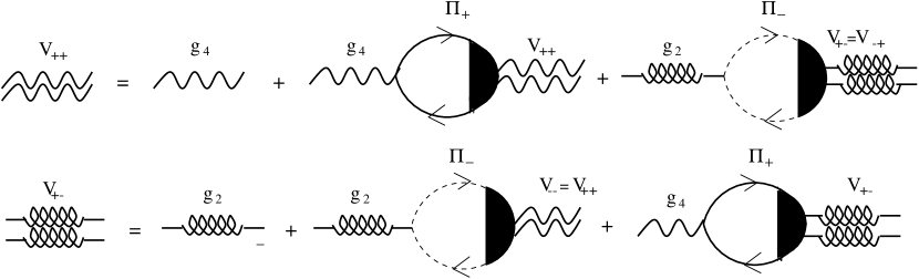
Fig. 11.: Dyson equation for the effective interaction. Solid line: Green’s function of a right-moving fermion. Dashed line: Green’s function of a left-moving fermion. Single wavy line: bare interaction of fermions of the same chirality; spiral line: same for the fermions of opposite chirality. Double wavy and spiral lines represent the renormalized interactions.

Effective interaction is obtained by collecting polarization corrections to the bare one. Diagrammatically, this procedure is described by the Dyson equation, represented in Fig.11. The interaction and polarization bubble are matrices with components

$$\hat{V}=\left(\begin{array}[]{cc}V_{++}&V_{+-}\\ V_{+-}&V_{++}\end{array}\right),\hat{V}_{0}=\left(\begin{array}[]{cc}g_{4}&g_{2}\\ g_{2}&g_{4}\end{array}\right),\hat{\Pi}=\left(\begin{array}[]{cc}\Pi_{+}&0\\ 0&\Pi_{-}\end{array}\right),$$

where we used an obvious symmetry $V_{++}=V_{--},V_{+-}=V_{-+}.$ The Dyson equation in the matrix form reads

$$\hat{V}=\hat{V}_{0}+\hat{V}_{0}\hat{\Pi}\hat{V},$$

or, in components,

$$V_{++} = g_{4}+g_{4}\Pi_{+}V_{++}+g_{2}\Pi_{-}V_{+-};$$

$$V_{+-} = g_{2}+g_{2}\Pi_{-}V_{++}+g_{4}\Pi_{-}V_{+-}.$$ (3.14)

The bubbles in these equations are fully renormalized ones, i.e., they are built on exact Green’s functions and contain a vertex (hatched corner):

$$\Pi_{\pm}\left(\omega,q\right)=-2i\int\int\frac{dkd\varepsilon}{\left(2\pi\right)^{2}}G_{\pm}\left(\varepsilon+\omega,k+q\right)G_{\pm}\left(\varepsilon,k\right)\Gamma_{\pm}^{0}\left(\varepsilon,k;\omega,q\right).$$

Now we use the Ward identity for $\Gamma_{\pm}^{0}$ (3.13) to get

$$\Pi_{\pm}\left(\omega,q\right)=-2i\frac{1}{\omega\mp q}\int\int\frac{dkd\varepsilon}{\left(2\pi\right)^{2}}\left[G_{\pm}\left(\varepsilon,k\right)-G_{\pm}\left(\varepsilon+\omega,k+q\right)\right].$$ (3.15)

Eq. (3.15) looks exactly the same as a free bubble [cf. Eq. (B. 2)] except that it contains exact rather than free Green’s functions. Because we managed to transform the product of two Green’s functions into a difference, frequency integration in Eq. (3.15) can be performed term by term yielding exact momentum distribution functions $n_{\pm}\left(k\right)$ and $n_{\pm}\left(k+q\right):$

$$\Pi_{\pm}\left(\omega,q\right)=\frac{1}{\omega\mp q}\int\int\frac{dk}{\pi}\left[n_{\pm}(k)-n_{\pm}(k+q)\right].$$ (3.16)

At the first glance, it seems that we have not achieved much so far. Indeed, we traded one unknown quantity ($\Pi_{\pm}$) for another ($n_{\pm}$). Both of them include the interaction to all orders and without any further simplification we are stuck. In fact, we have already made an important simplification: when specifying the model, we assumed only forward scattering. This means that the interaction is sufficiently long-range in real space so that backscattering can be neglected. Equivalently, in the momentum space it means that our interaction operates only in a narrow window of width $q_{0}$ near the Fermi points, $\pm k_{F}.$ Thus the states far away from the Fermi points are not affected by the interaction. The momentum integral in (3.16) comes from regions far away from the Fermi surface where unknown functions $n_{\pm}$ can be approximated by free Fermi steps. This approximation is good as long as $q_{0}\ll k_{F}.$ The solution is going to be exact only in a sense that there will be no constraints on the amplitude of the interaction (parameters $g_{2}$ and $g_{4})$ but not its range.Now we understand better why the title of the paper by Dzyaloshinskii and Larkin [59] is “Correlation functions for a one-dimensional Fermi system with long-range interaction (Tomonaga model)”.

With this simplification, the momentum integration proceeds in the same way as for free fermions (see Appendix Appendix B) with the result that the fully interacting bubbles are the same as free ones

$$\Pi_{\pm}\left(\omega,q\right)=\Pi_{\pm}^{0}\left(\omega,q\right)=\pm\frac{1}{\pi}\frac{q}{\omega-q+i0^{+}\mathrm{sgn}\omega}.$$ (3.17)

This is a truly remarkable result which is a cornerstone for the DL solution .

Because our bubbles were effectively “liberated” from the interaction effects, system (3.14) is equivalent to what we would have obtained from the Random Phase Approximation (RPA). It turns out that RPA is asymptotically exact in 1D in the limit $q_{0}/k_{F}\rightarrow 0.$ Solving the 2 by 2 system, we obtain for the effective interaction

$$V_{++}\left(\omega,q\right)=\left(\omega-q\right)\frac{g_{4}\left(\omega+q\right)+\left(g_{4}^{2}-g_{2}^{2}\right)q/\pi}{\omega^{2}-u^{2}q^{2}+i0^{+}},$$

where

$$u=\sqrt{1+\frac{2g_{4}}{\pi}+\frac{g_{4}^{2}-g_{2}^{2}}{\pi}}.$$

For $g_{4}=g_{2}\equiv g,$

$$V_{++}\left(\omega,q\right)=g\frac{\omega^{2}-q^{2}}{\omega^{2}-u^{2}q^{2}+i0^{+}}.$$ (3.18)

3.5 Dyson equation for the Green’s function

The Dyson equation for right-moving fermions reads

$$\Sigma_{+}\left(P\right)=i\int\frac{d^{2}Q}{\left(2\pi\right)^{2}}G_{+}\left(P-Q\right)V_{++}\left(Q\right)\Gamma_{+}^{0}\left(P,Q\right).$$

Diagrammatically, this equation is shown in Fig. 12.

Fig. 12.: Dyson equation for the self-energy.

For linear dispersion,

$$\Sigma_{\pm}\left(\varepsilon,p\right)=\varepsilon\mp p-G_{\pm}^{-1}\left(\varepsilon,p\right)$$

Substituting this relation back into the Dyson equations, we obtain

$$\left(\varepsilon-p\right)G_{+}\left(\varepsilon,p\right)=1+i\int\int\frac{d\omega dq}{\left(2\pi\right)^{2}}G_{+}\left(\varepsilon,p\right)G_{+}\left(\varepsilon-\omega,p-q\right)V_{++}\left(\omega,q\right)\Gamma_{+}^{0}\left(\varepsilon,p;\omega,q\right).$$

Using the Ward identity (3.13) , we get

$$\left(\varepsilon-p+\Sigma_{0}\right)G_{+}\left(\varepsilon,p\right)=1+i\int\int\frac{d\omega dq}{\left(2\pi\right)^{2}}G_{+}\left(\varepsilon,p\right)G_{+}\left(\varepsilon-\omega,p-q\right)$$

$$\times\frac{V_{++}\left(\omega,q\right)}{\omega-q}\left[G_{+}^{-1}\left(\varepsilon,p\right)-G_{+}^{-1}\left(\varepsilon-\omega,p-q\right)\right]$$

$$=1+i\int\int\frac{d\omega dq}{\left(2\pi\right)^{2}}G_{+}\left(\varepsilon-\omega,p-q\right)\frac{V_{++}\left(\omega,q\right)}{\omega-q}+G_{+}\left(\varepsilon,p\right)\times\mathrm{const,}$$

where

$$\mathrm{const=}i\int\int\frac{d\omega dq}{\left(2\pi\right)^{2}}\frac{V_{++}\left(\omega,q\right)}{\omega-q}$$

. A constant term can always be absorbed into $\Sigma,$ which simply results in a shift of the chemical potential. We are free to choose this shift in such a way that const=0, so that the Dyson equation reduces to

$$\left(\varepsilon-p\right)G_{+}\left(\varepsilon,p\right)=1+i\int\int\frac{d\omega dq}{\left(2\pi\right)^{2}}G_{+}\left(\varepsilon-\omega,p-q\right)\frac{V_{++}\left(\omega,q\right)}{\omega-q}.$$ (3.19)

Notice that Eq. (3.19) is an integral equation with a difference kernel, which can be reduced to a differential equation for $G.$ Before we demonstrate how it is done, let’s have a brief look at a case when there is no coupling between left- and right-moving fermions: $g_{2}=0.$ In this case,

$$V_{++}\left(\omega,q\right)=\pi\frac{\left(w-1\right)\left(\omega-q\right)}{\omega-wq+i0^{+}},$$

where

$$w=1+g_{4}/\pi.$$

Eq. (3.19) takes the form

$$\left(\varepsilon-p\right)G_{+}\left(\varepsilon,p\right)=1+i\left(w-1\right)\int\int\frac{d\omega dq}{4\pi}\frac{G_{+}\left(\varepsilon-\omega,p-q\right)}{\omega-wq+i0^{+}}.$$

This equation is satisfied by the following function

$$G_{+}\left(\varepsilon,p\right)=\frac{1}{\sqrt{\varepsilon-p+i0^{+}}\sqrt{\varepsilon-wp+i0^{+}}}.$$ (3.20)

This is an example of a non-Fermi-liquid behavior: the pole of a free $G$ splits into the product of two branch cuts, one peaked on the mass shell of free fermions ($\varepsilon=p)$ and another one at the renormalized mass shell ($\varepsilon=wp$). As left- and right movers are totally decoupled in this problem, the same result would have been obtained for two separate subsystems of left- and right movers. For example, Eq. (3.20) predicts that an edge state of an integer quantum Hall system is not a Fermi liquid, if spins are not yet polarized by the magnetic field [63]. The same procedure for a spinless system would give us a pole-like $G$ with a renormalized Fermi velocity. The non-Fermi-liquid behavior described by Eq. (3.20) is rather subtle: it exists only if both $\varepsilon$ and $p$ are finite. In the limiting case of $p=0$ (tunneling DoS) we are back to a free-fermion behavior $G\left(\varepsilon,0\right)=\varepsilon^{-1}.$ Also, the $\varepsilon-$ integral of Eq. (3.19) gives a step-like distribution function in momentum space. The spectral function, however, is characteristically non-FL-like: instead of delta-function peak we have a whole region $\left|p\right|<\left|\varepsilon\right|<w\left|p\right|$ in which Im$G$ is finite. At the edges of this interval Im$G$ has square-root singularities.

3.6 Solution for the case $g_{2}=g_{4}$

Substituting the effective interaction (3.18) into Dyson equation (3.19), we obtain

$$\left(\varepsilon-p\right)G_{+}\left(\varepsilon,p\right)=1+i\int\frac{d\omega dq}{4\pi^{2}}G\left(\varepsilon-\omega,p-q\right)g\left(q\right)\frac{\omega+q}{\omega^{2}-u^{2}q^{2}},$$

where

$$u=\sqrt{1+2g/\pi}.$$

Notice that the constant $g$ is replaced by a momentum-dependent interaction, $g\left(q\right).$ The reason is that without such a replacement the integral diverges at the upper limit. Here, the assumption of a cut-off in the interaction becomes important again. Transforming back to real time and space

$$G\left(x,t\right)=\int\int\frac{d\varepsilon dp}{\left(2\pi\right)^{2}}G\left(\varepsilon,p\right)e^{i\left(px-\varepsilon t\right)},$$

we obtain the Dyson equation in a differential form

$$\left(\frac{\partial}{\partial t}+\frac{\partial}{\partial x}\right)G\left(x,t\right)=P\left(x,t\right)G\left(x,t\right)-i\delta\left(x)\delta(t\right),$$ (3.21)

where

$$P\left(x,t\right)=\frac{1}{4\pi^{2}}\int\int d\omega dqe^{i\left(qx-\omega t\right)}g\left(q\right)\frac{\omega+q}{\omega^{2}-u^{2}q^{2}+i0^{+}}.$$ (3.22)

The integral for $P$ diverges if $g$ is constant. To ensure convergence, we will approximate $g\left(q\right)=ge^{-\left|q\right|/q_{0}}.$ An actual form of the cut-off function is not important as long as we are interested in such times and spatial intervals such that $x,t\gg q_{0}^{-1}.$ The integral over $\omega$ is solved by closing the contour around the poles of the denominator $\omega=\pm u\left|q\right|\left(1+i0^{+}\right).$ For $t>0,$ we need to choose the one with Im$\omega<0.$ Doing so, we obtain

$$\int\frac{d\omega}{2\pi}\dots=i\frac{\mathrm{sgn}q+u}{2u}e^{i\left(qx-u\left|qt\right|\right)}.$$

Solving the remaining $q-$ integral, we obtain for $P\left(x,t\right)$

$$P\left(x,t\right)=\frac{g}{4\pi u}\left(\frac{u+1}{x-ut+i/q_{0}}-\frac{u-1}{x+ut+i/q_{0}}\right).$$

For $t<0,$ one needs to change $q_{0}\rightarrow-q_{0}$ in the last formula.

The delta-function term can be viewed as a boundary condition

$$G\left(x,0+\right)-G\left(x,0-\right)=-i\delta\left(x\right).$$ (3.23)

Once the function $P\left(x,t\right)$ is known, Eq. (3.21) is trivially solved in terms of new variables $r=x-t,$ $s=x+t.$ For example, for $t>0$

$$G_{+}\left(r,t>0\right)=G_{0}\left(x,t\right)f_{>}\left(r\right)\exp\left[i\int_{r}^{s}ds^{\prime}P\left(r,s^{\prime}\right)\right],$$ (3.24)

where function $f_{>}(r)$ is determined by the analytic properties of $G$ as a function of $\varepsilon.$ Substituting result for $P\left(x,t\right)$ into Eq. (3.24), we get

$$G_{+}\left(x,t>0\right)=\frac{1}{2\pi}G_{0}\left(x,t\right)f_{>}\left(x-t\right)\left(\frac{x-t+i/q_{0}}{x-ut+i/q_{0}}\right)^{\alpha+1/2}\left(\frac{x-t-i/q_{0}}{x+ut-i/q_{0}}\right)^{\alpha}.$$

where

$$\alpha=\frac{\left(u-1\right)^{2}}{8u}.$$ (3.25)

Formula for $t<0$ is obtained by choosing another function $f_{<}$ and replacing $q_{0}\rightarrow-q_{0}.$ Functions $f_{>,<}$ are determined from the analytic properties. First of all, recall that

$$G_{0}\left(x,t\right)=\frac{1}{x-t+i\mathrm{sgn}t0^{+}}.$$

We see that although $G_{0}$ is not an analytic function of $t$ for any $t,$ it is analytic for Re$t>0$ in the right lower quadrant (Im$t<0)$ and for Re$t<0$ in the upper left quadrant (Im$t>0$). The interaction cannot change analytic properties of a Green’s function hence we should expect the same properties to hold for full $G.$

From the boundary condition (3.23), it follows that

$$f_{>}\left(x\right) = f_{<}\left(x\right)$$

$$\mathrm{and}\;f\left(0\right) = 0.$$

Analyzing different factors in the formula for $G,$ we see that only the term $\left(x-t\mp i/q_{0}\right)^{\alpha}$ does not satisfy the required analyticity property. This term is eliminated by choosing function $f\left(x\right)$ as

$$f\left(x\right)=\left(q_{0}^{2}x^{2}+1\right)^{-\alpha}.$$

Finally, the result for $G$ takes the form

$$G_{+}\left(x,t\right) = \frac{1}{2\pi}\frac{1}{x-t+i\mathrm{sgn}t0^{+}}\left(\frac{x-t+i\gamma}{x-ut+i{\gamma}}\right)^{1/2}$$

$$\times\frac{1}{\left[q_{0}^{2}\left(x-ut+i{\gamma}\right)\left(x+ut-i{\gamma}\right)\right]^{\alpha}},$$

where $\gamma=\mathrm{sgn}t/q_{0}.$ It seems somewhat redundant to keep two different damping terms ($i\mathrm{sgn}t0^{+}$ and $\gamma)$ in the same equation. However, these terms contain different physical scales. Indeed, $i\mathrm{sgn}t0^{+}$ enters a free Green’s function and $0^{+}$ there has to be understood as the limit of the inverse system size. On the other hand, $\gamma$ contains a cut-off of the interaction. Obviously, $|\gamma|\gg 1/L\rightarrow 0^{+}$ for a realistic situation. The difference between the two cutoffs becomes important for the momentum distribution function and tunneling DoS, discussed in the next Section.

3.7 Physical properties

3.7.1 Momentum distribution

Having an exact form of the Green’s function, we can now calculate the momentum distribution of, e.g., right-moving fermions:

$$n_{+}\left(p\right) = -i\int_{-\infty}^{\infty}dxe^{-ipx}G_{+}\left(x,t\rightarrow 0^{+}\right)$$

$$= -\frac{i}{2\pi}\int_{-\infty}^{\infty}dx\frac{e^{-ipx}}{x+i0^{+}}\frac{1}{\left[q_{0}^{2}x^{2}+1\right]^{\alpha}}$$

$$= -\frac{i}{2\pi}\int_{-\infty}^{\infty}dxe^{-ipx}\left[\mathcal{P}\frac{1}{x}-i\pi\delta\left(x\right)\right]\frac{1}{\left[q_{0}^{2}x^{2}+1\right]^{\alpha}}$$

$$= \frac{1}{2}-\frac{1}{\pi}\text{sgn}p\int_{0}^{\infty}dx\frac{\sin\left|p\right|x}{x}\frac{1}{\left[q_{0}^{2}x^{2}+1\right]^{\alpha}},$$

We are interested in the behavior at $p\rightarrow 0$ (which means $\left|p\right|\ll q_{0}).$ The final result for $n_{+}\left(p\right)$ depends on whether $\alpha$ is larger or smaller than $1/2$ [59, 64].

• For $\alpha<1/2$ (“weak interaction”), one cannot expand $\sin px$ in $x$ because the resulting integral diverges at $x=\infty.$ Instead, rescale $px\rightarrow y$

  $$n_{+}\left(p\right)=\frac{1}{2}-\frac{1}{\pi}\int_{0}^{\infty}dy\frac{\sin y}{y}\frac{1}{\left[\left(q_{0}/p\right)^{2}y^{2}+1\right]^{\alpha}}$$

  and neglect $1$ in the denominator. This gives

  $$n_{+}\left(p\right)=\frac{1}{2}+C_{1}\left(\frac{\left|p\right|}{q_{0}}\right)^{2\alpha}\text{sgn}p$$ (3.26)

  where

  $$C_{1}=\frac{\sin\pi\alpha}{\pi}\Gamma\left(-2\alpha\right).$$

  Notice that $n_{+}\left(p\right)$ is finite ($=1/2$) at $p=0,$ although its derivative is singular. We should be able to recover the Fermi-gas step at $p=0$ by setting $\alpha=0$ in (3.26). Indeed,

  $$\lim_{\alpha\rightarrow 0}C_{1}=\alpha\frac{1}{-2\alpha}=-\frac{1}{2}$$

  and

  $$n\left(p\right)=\frac{1-\text{sgn}p}{2},$$

  which is just the Fermi-gas result. Notice also that there is nothing special about the limit $\alpha\rightarrow 0$ . Indeed, constant $C_{1}$ has a regular expansion in $\alpha$

  $$C_{1}=-\frac{1}{2}-\gamma\alpha+\dots,$$

  where $\gamma=0.577\dots$ and factor $\left(\left|p\right|/q_{0}\right)^{2\alpha}$ can be expanded for finite $p$ and small $\alpha$ as

  $$\left(\left|p\right|/q_{0}\right)^{2\alpha}=1+2\alpha\ln\left|p\right|/q_{0}.$$

  To leading order in $\alpha$, we obtain

  $$n_{+}\left(p\right)=\frac{1}{2}-\text{sgn}p\frac{1}{2}\left[1+2\alpha\ln\left|p\right|/q_{0}\right]=n_{0}\left(p\right)-\alpha\text{sgn}p\ln\left|p\right|/q_{0},$$

  which is a perfectly regular in $\alpha$ (but logarithmically divergent at $p\rightarrow 0)$ behavior. Once again, it is not surprising: despite the fact that the results for a 1D system differ dramatically from that for the Fermi gas, they are still perturbative, i.e., analytic, in the coupling constant.

• For $\alpha>1/2$ (“strong interaction”), it is safe to expand $\sin px$ and the result is

  $$n_{+}\left(p\right)=\frac{1}{2}-C_{2}p/q_{0},$$

  where

  $$C_{1}=\frac{1}{2\sqrt{\pi}}\frac{\Gamma\left(\alpha-1/2\right)}{\Gamma\left(\alpha\right)}.$$

  In this case, no remains of a jump at the Fermi point is present in $n_{+}\left(p\right)$ which is a regular, linear function near $p=0.$

• Finally, $\alpha=1/2$ is a special case, where expansion in $p$ results in a log-divergent integral. To log-accuracy

  $$n_{+}\left(p\right)=\frac{1}{2}-\frac{1}{\pi}\frac{p}{q_{0}}\ln\frac{q_{0}}{\left|p\right|}.$$

In general, $n\left(p\right)$ is some hypergeometric function of $p/q_{0}$ which decays rapidly for $p\gg q_{0}$ and approaches $1$ for $p\ll-q_{0}$. A posteriori, this justifies the replacement of exact $n\left(p\right)$ by its free form in the Dyson equation.

3.7.2 Tunneling density of states

Now we turn to the tunneling DoS

$$N\left(\varepsilon\right)=-\frac{1}{\pi}\mathrm{Im}G^{R}\left(\varepsilon,x=0\right).$$

Recalling that [23]

$$G^{R}\left(\varepsilon\right) = G\left(\varepsilon\right),\mathrm{for}\text{ }\mathrm{\varepsilon>0;}$$

$$= G^{\ast}\left(\varepsilon\right),\mathrm{\ for}\text{ }\mathrm{\varepsilon<0,}$$

we see that

$$\mathrm{Im}G^{R}\left(\varepsilon,0\right)=\text{sgn}\varepsilon\mathrm{Im}G\left(\varepsilon,0\right)$$

and

$$N\left(\varepsilon\right) = -\frac{1}{\pi}\text{sgn}\varepsilon\mathrm{Im}G\left(0,\varepsilon\right)=-\frac{1}{\pi}\text{sgn}\varepsilon\left[\int dte^{i\varepsilon t}G\left(0,t\right)-\int dte^{-i\varepsilon t}G^{\ast}\left(0,t\right)\right]$$

$$= -\frac{1}{\pi}\text{sgn}\varepsilon\left[\int dte^{i\varepsilon t}\left\{G\left(0,t\right)-G^{\ast}\left(0,-t\right)\right\}\right]$$

For $t\rightarrow\infty,$

$$G\left(0,t\right)=\frac{\text{const}}{\left(-t\right)^{1+2\alpha}}$$

and

$$G\left(0,t\right)-G^{\ast}\left(-t\right)$$

is an odd function of $t.$ Thus

$$N\left(\varepsilon\right) = -\frac{1}{\pi}\text{sgn}\varepsilon\mathrm{Im}G\left(0,\varepsilon\right)=-\frac{1}{\pi}\text{sgn}\varepsilon\frac{1}{2i}\left[\int dte^{i\varepsilon t}G\left(0,t\right)-\int dte^{-i\varepsilon t}G^{\ast}\left(0,t\right)\right]$$

$$= -\frac{1}{\pi}\text{sgn}\varepsilon\left[\int_{0}^{\infty}dt\sin\varepsilon t\left\{G\left(0,t\right)-G^{\ast}\left(0,-t\right)\right\}\right]\propto\text{sgn}\varepsilon\int_{0}^{\infty}dt\frac{\sin\varepsilon t}{t^{1+2\alpha}}.$$

The integral is obviously convergent for $\alpha<1/2.$ In this case,

$$N_{s}\left(\varepsilon\right)\propto\left|\varepsilon\right|^{2\alpha},$$

which means that the local tunneling DoS is suppressed at the Fermi level. Actually, the exponent for $\alpha>1/2$ is the same, however, the prefactor is a different function of $\alpha$ [65].

The DoS in Eq. (3.7.2) with exponent $2\alpha$, where $\alpha$ is given by Eq. (3.25) corresponds to tunneling into the “bulk” of a 1D system, i.e., when the tunneling contact (with a tip of an STM or another carbon nanotube crossing the first one) is far away from its ends. In the next Section, we will analyze tunneling into an edge of a 1D conductor, which is characterized by a different exponent, $\alpha^{\prime}$.

4 Renormalization group for interacting fermions

The Tomonaga-Luttinger model can be solved exactly as it was done in the previous Section– only in the absence of backscattering. Backscattering can be treated via the Renormalization Group (RG) procedure. This treatment is standard by now and discussed in a number of sources [1, 2, 3, 4, 5, 6, 7, 8, 9, 10]. For the sake of completeness, I present here a short derivation of the RG equations. A reader familiar with the procedure can skip this Section and go directly to Sec. 5, where these equations will be used in the context of a single-impurity problem.

An exact solution of the previous Section is parameterized by two coupling constants, $g_{2}$ and $g_{4}$, which are equal to their bare values. In the RG language, it means that these couplings do not flow. Let’s see if this is indeed the case. In what follows, I will neglect the $g_{4}-$ processes, as their effect on the flow of other couplings is trivial, and, for the sake of simplicity, consider a spin-independent interaction. To second order, the renormalization of the $g_{2}-$ coupling is accounted for by two diagrams: diagrams a) and b) of Fig. 13.

Diagram a) is a correction to $g_{2}$ in the particle-particle channel. The correction to $g_{2}$ is given by

$$\left(g_{2}^{\left(2\right)}\right)_{a}=\frac{g_{2}^{2}}{\left(2\pi\right)^{2}}\int dq\int d\omega G_{+}\left(i\varepsilon_{1}+i\omega,k_{1}+q\right)G_{-}\left(i\varepsilon_{2}-i\omega,k_{2}-q\right).$$

Without a loss of generality, one can choose all momenta to be on the Fermi “surface”: $k_{1}=k_{2}=k_{3}=k_{4}=0.$ Choose $q>0$ (the other choice $q<0$ will simply double the result)

$$\left(g_{2}^{\left(2\right)}\right)_{a} = \frac{g_{2}^{2}}{\left(2\pi\right)^{2}}\int dq\int d\omega G_{+}\left(i\varepsilon_{1}+i\omega,q\right)G_{-}\left(i\varepsilon_{2}-i\omega,-q\right)$$

$$= \frac{g_{2}^{2}}{\left(2\pi\right)^{2}}\int_{0}^{\Lambda/2}dq\int d\omega\frac{1}{i\left(\varepsilon_{1}+\omega\right)-q}\frac{1}{i\left(\varepsilon_{2}-\omega\right)-q}$$

$$= \frac{2\pi ig_{2}^{2}}{\left(2\pi\right)^{2}}\int_{0}^{\Lambda/2}dq\frac{1}{\varepsilon_{1}+\varepsilon_{2}+\omega+2iq}=\frac{g_{2}^{2}}{4\pi}\ln\frac{i\Lambda}{\varepsilon_{1}+\varepsilon_{2}}$$

Adding the result up with the (identical) $q<0$ contribution, we find

$$\left(g_{2}^{\left(2\right)}\right)_{a}=\frac{g_{2}^{2}}{2\pi}\ln\frac{i\Lambda}{\varepsilon_{1}+\varepsilon_{2}}.$$

Diagram b) is a correction to $g_{2}$ in the particle-hole channel:

$$\left(g_{2}^{\left(2\right)}\right)_{b} = \frac{g_{2}^{2}}{\left(2\pi\right)^{2}}\int dq\int d\omega G_{+}\left(i\varepsilon_{1}+i\omega,q\right)G_{-}\left(i\varepsilon_{4}+i\omega,q\right)$$

$$= \frac{g_{2}^{2}}{\left(2\pi\right)^{2}}\int_{0}^{\Lambda/2}dq\int d\omega\frac{1}{i\left(\varepsilon_{1}+\omega\right)-q}\frac{1}{i\left(\varepsilon_{4}+\omega\right)+q}$$

$$= -\frac{2\pi i}{\left(2\pi\right)^{2}}g_{2}^{2}\int_{0}^{\mathbf{\Lambda}/2d}q\frac{1}{\varepsilon_{1}-\varepsilon_{4}+\omega+2iq}=-\frac{g_{2}^{2}}{4\pi}\ln\frac{i\Lambda}{\varepsilon_{1}-\varepsilon_{4}}.$$

As in the previous case, the final result is:

$$\left(g_{2}^{\left(2\right)}\right)_{b}=-\frac{g_{2}^{2}}{2\pi}\ln\frac{i\Lambda}{\varepsilon_{1}-\varepsilon_{4}}.$$

Fig. 13.: Second order diagrams for couplings $g_{2}$ (solid wavy line) and $g_{1}$ (dashed wavy line). Straight solid and dashed lines correspond to Green’s functions of right- and left moving fermions, correspondingly.

If we sum only the Cooper ladders, adding up more vertical interaction lines to diagram a), the full vertex becomes

$$\Gamma_{pp}=\frac{g_{2}}{1+g_{2}\ln\frac{i\Lambda}{\varepsilon_{1}+\varepsilon_{2}}}.$$

(To keep track of the signs, one needs to recall that in Matsubara frequencies each interaction line comes with the minus sign from the expansion of the $S-$ matrix). The resulting vertex blows up for attractive interaction ($g_{2}<0$) as $\varepsilon_{1}+\varepsilon_{2}\rightarrow 0,$ which is nothing more than a Cooper instability.

Likewise, untwisting the crossed lines in diagram b) and adding more interaction lines, we get the particle-hole vertex

$$\Gamma_{ph}=\frac{g_{2}}{1-g_{2}\ln\frac{i\Lambda}{\varepsilon_{1}-\varepsilon_{4}}}.$$

This vertex has an instability for repulsive interaction ($g_{2}>0).$ In fact, none of these instabilities occur. To see this, add up the results of diagrams a) and b)

$$\left(g_{2}^{\left(2\right)}\right)_{a+b}=\frac{g_{2}^{2}}{2\pi}\left[\ln\frac{i\Lambda}{\varepsilon_{1}+\varepsilon_{2}}-\ln\frac{i\Lambda}{\varepsilon_{1}-\varepsilon_{4}}\right]=\frac{g_{2}^{2}}{2\pi}\ln\frac{\varepsilon_{1}-\varepsilon_{4}}{\varepsilon_{1}+\varepsilon_{2}}.$$

In the RG, one changes the cut-off and follow the corresponding evolution of the couplings. As the cut-off dependence cancelled out in the result for $\left(g_{2}^{\left(2\right)}\right)_{a+b},$ coupling $g_{2}$ remains invariant under the RG flow.

Backscattering generates additional diagrams: diagrams c)-f) in Fig.13.

Diagram c) describes repeated backscattering in the particle-particle channel, which is equivalent to forward scattering. Therefore, this diagram gives a correction to $g_{2}-$ coupling. Using the relation between $G_{\pm}$, i.e., $G_{\pm}=-\left(G_{\mp}\right)^{\ast},$ we find

$$\left(g_{2}^{\left(2\right)}\right)_{c} = \frac{g_{1}^{2}}{\left(2\pi\right)^{2}}\int dq\int d\omega G_{-}\left(i\varepsilon_{1}+i\omega,q\right)G_{+}\left(i\varepsilon_{4}+i\omega,q\right)$$

$$= \frac{g_{1}^{2}}{\left(2\pi\right)^{2}}\left[\int dq\int d\omega G_{+}\left(i\varepsilon_{1}+i\omega,q\right)G_{-}\left(i\varepsilon_{4}+i\omega,q\right)\right]^{\ast}.$$

The last integral is the same as for $\left(g_{2}^{\left(2\right)}\right)_{a}.$ Thus,

$$\left(g_{2}^{\left(2\right)}\right)_{c}=\frac{g_{1}^{2}}{g_{2}^{2}}\left[dg_{2}^{\left(1\right)}\right]^{\ast}=\frac{g_{1}^{2}}{2\pi}\ln\frac{-i\Lambda}{\varepsilon_{1}+\varepsilon_{2}}.$$

The rest of the diagrams provide corrections to $g_{1}.$

Diagram d1)  is the same as diagram a) except for the prefactor being equal to $g_{1}g_{2}:$

$$\left(g_{1}^{\left(2\right)}\right)_{d1}=\frac{g_{1}g_{2}}{2\pi}\ln\frac{i\Lambda}{\varepsilon_{1}+\varepsilon_{2}}$$

Diagram d2) is a complex-conjugate of diagram d1). The sum of diagrams d1) and d2) is equal to  

$$\left(g_{1}^{\left(2\right)}\right)_{d1+d2} = \frac{g_{1}g_{2}}{2\pi}\ln\frac{i\Lambda}{\varepsilon_{1}+\varepsilon_{2}}+\frac{g_{1}g_{2}}{2\pi}\ln\frac{-i\Lambda}{\varepsilon_{1}+\varepsilon_{2}}$$

$$= \frac{g_{1}g_{2}}{\pi}\ln\frac{\Lambda}{\varepsilon_{1}+\varepsilon_{2}}.$$

Diagrams e) is a polarization correction to the bare $g_{1}-$coupling:

$$\left(g_{1}^{\left(2\right)}\right)_{e}=\underbrace{-}_{\text{{fermionic loop}}}g_{1}^{2}\Pi_{2k_{F}}\left(\omega=\varepsilon_{1}-\varepsilon_{2},q=0\right).$$

Using Eq. (B. 8), we obtain

$$\left(g_{1}^{\left(2\right)}\right)_{e}=\frac{N_{s}}{2\pi}g_{1}^{2}\ln\frac{\Lambda}{\left|\varepsilon_{1}-\varepsilon_{2}\right|},$$

where $N_{s}$ is the degeneracy factor (=2 for spin 1/2 fermions, occupying a single valley in the momentum space).

Diagram f1) is the same as the bubble insertion, except for no minus sign, no degeneracy factor ($N_{s})$ factor, and the overall coefficient is $g_{1}g_{2:}$

$$\left(g_{1}^{\left(2\right)}\right)_{f1}=-\frac{1}{2\pi}g_{1}g_{2}\ln\frac{\Lambda}{\left|\varepsilon_{1}-\varepsilon_{2}\right|}.$$

Diagram f2) is equal to f1). Their sum  

$$\left(g_{1}^{\left(2\right)}\right)_{f1+f2}=-\frac{1}{\pi}g_{1}g_{2}\ln\frac{\Lambda}{\left|\varepsilon_{1}-\varepsilon_{2}\right|}$$

Collecting all contributions together, we obtain

$$-\Gamma_{2} = -g_{2}+\left(g_{2}^{\left(2\right)}\right)_{a}+\left(g_{2}^{\left(2\right)}\right)_{b}+\left(g_{2}^{\left(2\right)}\right)_{c};$$

$$\Gamma_{2} = g_{2}\underbrace{-\frac{g_{2}^{2}}{2\pi}\ln\frac{i\Lambda}{\varepsilon_{1}+\varepsilon_{2}}+\frac{g_{2}^{2}}{2\pi}\ln\frac{i\Lambda}{\varepsilon_{1}-\varepsilon_{4}}}_{\text{{cancel out in the RG sense}}}-\frac{g_{1}^{2}}{2\pi}\ln\frac{-i\Lambda}{\varepsilon_{1}+\varepsilon_{2}};$$

$$-\Gamma_{1} = -g_{1}+\left(g_{2}^{\left(2\right)}\right)_{d}+\left(g_{2}^{\left(2\right)}\right)_{e}+\left(g_{2}^{\left(2\right)}\right)_{f};$$

$$\Gamma_{1} = g_{1}-\frac{g_{1}g_{2}}{\pi}\ln\frac{\Lambda}{\varepsilon_{1}+\varepsilon_{2}}-\frac{N_{s}}{2\pi}g_{1}^{2}\ln\frac{\Lambda}{\left|\varepsilon_{1}-\varepsilon_{2}\right|}+\frac{1}{\pi}g_{1}g_{2}\ln\frac{\Lambda}{\left|\varepsilon_{1}-\varepsilon_{2}\right|}.$$

Second and fourth terms in $\Gamma_{1}$ also cancel out in the RG sense. Changing the cut-off from $\Lambda$ to $\Lambda+d\ \Lambda$, we obtain two differential equations

$$\frac{d\Gamma_{2}}{dl} = -\frac{\Gamma_{1}^{2}}{2\pi};$$ (4.1)

$$\frac{d\Gamma_{1}}{dl} = -N_{s}\frac{\Gamma_{1}^{2}}{2\pi},$$ (4.2)

where $l=\ln\Lambda.$ We see that a quantity

$$\bar{\Gamma}=\Gamma_{2}-\frac{1}{N_{s}}\Gamma_{1}=\text{const}=g_{2}-\frac{1}{N_{s}}g_{1}.$$ (4.3)

is invariant under RG flow, therefore its value can be obtained by substituting the bare values of the coupling constants ($g_{2}$ and $g_{1})$ into (4.3). The RG-invariant combination is then

$$\bar{\Gamma}=g_{2}-\frac{1}{N_{s}}g_{1}.$$ (4.4)

For spinless electrons ($N_{s}=1)$,

$$\bar{\Gamma}=\Gamma_{2}-\Gamma_{1}=U\left(0\right)-U\left(2k_{F}\right).$$

This last result can be understood just in terms of the Pauli principle. Indeed, the anti-symmetrized vertex for spinless electrons is obtained by switching the outgoing legs of the diagram ($p_{1},p_{2}\rightarrow p_{3},p_{4}).$ To first order,

$$\Gamma\left(p_{1},p_{2};p_{3},p_{4}\right)=U\left(p_{1}-p_{3}\right)-U\left(p_{1}-p_{4}\right).$$

Choosing $p_{3}=p_{1}-q$ and $p_{4}=p_{2}+q,$ we obtain [recall that $U\left(q\right)=U\left(-q\right)]$

$$\Gamma\left(p_{1},p_{2}|q\right)=U\left(q\right)-U(p_{1}-p_{2}-q).$$

One of the incoming fermions is a right mover ($p_{1}=p_{F}$) and the other one is a left mover ($p_{2}=-p_{F}$). As $q$ is small compared to $p_{F},$ we obtain

$$\Gamma\left(p_{1},p_{2}|q\right)=U\left(0\right)-U(2k_{F}).$$

In fact, for spinless electrons $g_{2}$ and $g_{1}$ processes are indistinguishable as we do not know whether the right-moving electron in the final state is a right-mover of the initial state, which experienced forward scattering, or the left-mover of the initial state, which experienced backscattering. A proper way to treat the case of spinless fermions is to include backscattering into Dzyaloshinskii-Larkin scheme from the very beginning, re-write the Hamiltonian in terms of forward scattering with invariant coupling $\bar{\Gamma},$ and proceed with the solution. All the results will then be expressed in terms of $\bar{\Gamma}$ rather than of $g_{2}.$

Solving the equation for $\Gamma_{1},$ gives on scale $\varepsilon$

$$\Gamma_{1}=\frac{1}{\left(g_{1}\right)^{-1}+\frac{N_{s}}{2\pi}\ln\Lambda/\varepsilon}.$$ (4.5)

At low energies, $\Gamma_{1}$ renormalizes to zero ($\Gamma_{1}^{\ast}=\Gamma_{1}\left(l=\infty\right)=0)$, if the interaction is repulsive, and blows up at $\varepsilon=\Lambda\exp\left(-1/|g_{1}|\right)$, if the interaction is attractive. Coupling $\Gamma_{2}$ also flows to a new value which can be read off from Eq. (4.4)

$$\Gamma_{2}^{\ast}=g_{2}-\frac{1}{N_{s}}g_{1}.$$

Roughly speaking, $g_{1}$ is not important for repulsive interaction as the effective low-energy theory will look like a theory with forward scattering only. This does not really mean, however, that one can consider a fixed point as a new problem in which backscattering is absent, and apply our exact solution to this problem. Instead, one should calculate observables, derive the RG equations for flows, and use current values of coupling constants in these RG equations. An example of this procedure will be given in the next Section, where we will see that the flow of $\Gamma_{1}$ provides additional renormalization of the transmission coefficient in an interacting system.

Assigning different coupling constants to the interaction of fermions of parallel ($g_{1||}$) and anti-parallel ($g_{1\perp}$) spins, one could see that the coupling which diverges for attractive interaction is in fact $g_{1\perp}.$ This clarifies the nature of the gap that RG hints at (in fact, a perturbative RG can at most just give a hint): it is a spin gap. This becomes obvious in the bosonization technique, as the instability occurs in the spin-sector of the theory. An exact solution by Luther and Emery [66] for a special case of attractive interaction confirms this prediction.

5 Single impurity in a 1D system: scattering theory for interacting fermions

A single impurity or tunneling barrier placed in a 1D Fermi gas reduces the conductance from its universal value–$e^{2}/h$ per spin orientation–to

$${\cal G}=N_{s}\frac{e^{2}}{h}|t_{0}|^{2},$$ (5.1)

where $t_{0}$ is the transmission amplitude. The interaction renormalizes the bare transmission amplitude. As a result, the conductance depends on the characteristic energy scale (temperature or applied bias), which is observed as a zero-bias anomaly in tunneling. This effect is not really a unique property of 1D : in higher dimensions, zero-bias anomalies in both dirty and clean (ballistic) regimes [67, 12, 13, 14] as well as the interaction correction to the conductivity [67, 15], stem from the same physics, namely, scattering of electrons from Friedel oscillations produced by tunneling barriers or impurities. 1D is special in the magnitude of the effect: the conductance varies significantly already on the energy scale comparable to the Fermi energy, whereas in higher dimensions the effect of the interaction is either small at all energies or becomes significant only at low energies (below some scale which is much smaller than $E_{F}$ as long as the parameter $k_{F}l$, where $l$ is the elastic mean free path, is large. The 1D zero-bias anomaly is described quite simply in a bosonized language [68], which does not require the interaction to be weak. We will use this description in Sec.6. However, in this Section I will choose another description–via the scattering theory for fermions rather than bosons–developed by Matveev, Yue, and Glazman [11]. Although this approach is perturbative in the interaction, it elucidates the underlying mechanism of the zero-bias anomaly and allows for an extension to higher-dimensional case (which was done for the case of tunneling in Ref.[12] and transport in Ref.[15]).

5.1 First-order interaction correction to the transmission coefficient

In this section we consider a 1D system of spinless fermions with a tunneling barrier located at $x=0$ [11]. For the sake of simplicity, I assume that the barrier is symmetric, so that transmission and reflection amplitude for the waves coming from the left and right are the same. Also, I assume that e-e interaction is present only to the right of the barrier, whereas to the left we have a Fermi gas. Such a situation models a setup when a tunneling contact separates a 1D interacting system (quantum wire or carbon nanotube) and a “good metal”, where one can be neglect the interaction. We also assume that the interaction potential $U\left(x\right)$ is sufficiently short-ranged, so that $U\left(0\right)$ is finite and one can neglect over-the-barrier interaction. However, $U\left(0\right)\neq U\left(2k_{F}\right)$ (otherwise, spinless electrons do not interact at all).

The wave function of the free problem for a right-moving state is:

$$\psi_{k}^{0}\left(x\right) = \frac{1}{\sqrt{L}}\left(e^{ikx}+r_{0}e^{-ikx}\right),x<0;$$

$$= \frac{1}{\sqrt{L}}t_{0}e^{ikx},x>0.$$

For a left-moving state:

$$\psi_{-k}^{0}\left(x\right) = \frac{1}{\sqrt{L}}\left(e^{-ikx}+r_{0}e^{ikx}\right),x>0;$$ (5.3)

$$= \frac{1}{\sqrt{L}}t_{0}e^{-ikx},x<0.$$

Here $k=\sqrt{2mE}>0.$ To begin with, we consider a high barrier: $\left|t_{0}\right|\ll 1,r_{0}\approx-1.$ Then the free wavefunction reduces to

$$\psi_{k}^{0}\left(x\right) = \frac{2i}{\sqrt{L}}\sin kx,x<0\;\;\text{{(incoming from the left+reflected);}}$$ (5.4)

$$= \frac{1}{\sqrt{L}}t_{0}e^{ikx},x>0\;\;\text{{(transmitted left}}\rightarrow\text{{\ right);}}$$ (5.5)

$$\psi_{-k}^{0}\left(x\right) = \frac{1}{\sqrt{L}}t_{0}e^{-ikx},x<0\;\;\text{{(transmitted right}}\rightarrow\text{{left);}}$$ (5.6)

$$= -\frac{2i}{\sqrt{L}}\sin kx,x>0\;\;\text{{(incoming from the right+reflected).}}$$ (5.7)

The barrier causes the Friedel oscillation in the electron density on both sides of the barrier. The interaction is treated perturbatively, via finding the corrections to the transmission coefficient due to additional scattering at the potential produced by the Friedel oscillation. Diagrammatically, the corrections to the Green’s function are described by the diagrams in Fig.14, where a) represents the Hartree and b) the exchange (Fock) contributions, correspondingly. Compared to the textbook case, though, the solid lines in these diagrams are the Green’s functions composed of the exact eigenstates in the presence of the barrier (but no interaction). Because the barrier breaks translational invariance, these Green’s functions are not translationally invariant as well. I emphasized this fact by drawing the diagrams in real space, as opposed to the momentum -space representation. Notice also that the Hartree diagram is usually discarded in textbooks because the bubble there corresponds to the total charge density (density of electrons minus that of ions), which is equal to zero in a translationally invariant and neutral system. However, what we have in our case is the local density of electrons at some distance from the barrier. Friedel oscillation is a relatively short-range phenomenon (the period of the oscillation is comparable to the electron wavelength), and it is possible to violate the charge neutrality locally on such a scale. As a result, the Hartree correction is not zero.

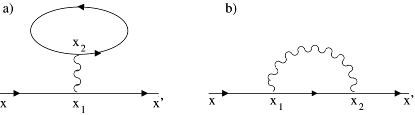
Fig. 14.: Correction to the Green’s function: exact with respect to the barrier and first order in the interaction.

To first-order in the interaction, an equivalent way of solving the problem is to find a correction to the wave-function, rather than the Green’s function, in the Hartree-Fock method. The electron wave-function which includes both the barrier potential and the electron-electron interaction is

$$\psi_{k}(x) = \psi_{k}^{0}(x)+\int_{0}^{\infty}dx^{\prime}G_{0}^{>}(x\mathbf{,}x^{\prime},E)$$ (5.8)

$$\times\int_{0}^{\infty}dx^{\prime\prime}[V_{H}(x^{\prime\prime})\delta(x^{\prime}-x^{\prime\prime})+V_{ex}(x^{\prime},x^{\prime\prime})]\psi_{k}^{0}\left(x^{\prime\prime}\right),$$

where $G_{0}^{>}$ is the Green’s function of free electrons on the right semi-line, $E$ is the full energy of an electron, $V_{H}$ and $V_{ex}$ are the Hartree and the exchange potentials. The Hartree potential is

$$V_{H}(x)=\int dx^{\prime}U(x-x^{\prime})\delta n(x^{\prime}),$$ (5.9)

where $\delta n(x)=n(x)-n_{0}$ is the deviation of the electron density from its uniform value (in the absence of the potential) and $U(x)$ is the interaction potential. Hartree interaction is a direct interaction with the modulation of the electron density by the Friedel oscillation. For a high barrier, which is essentially equivalent to a hard-wall boundary condition, the electron density is

$$n(x) = 4\int_{0}^{k_{F}}\frac{dk}{2\pi}\sin^{2}(kx)=n_{0}\left(1-\frac{\sin 2k_{F}x}{2k_{F}x}\right)\rightarrow$$ (5.10)

$$\delta n\left(x\right) = -\sin\left(2k_{F}x\right)/2\pi x,$$ (5.11)

where $n_{0}=k_{F}/\pi$ is the density of electrons. Then,

$$V_{H}(x)=-\frac{1}{2\pi}\int_{0}^{\infty}dx^{\prime}U(x-x^{\prime})\frac{\sin 2k_{F}x^{\prime}}{x^{\prime}}.$$ (5.12)

Notice that although the bare interaction is short-range, the effective interaction has a slowly-decaying tail due to the Friedel oscillation. (The integral goes over only for positive values of $x^{\prime}$ because electrons interact only there.)

The exchange potential is equal to

$$V_{ex}(x,x) = -U(x-x^{\prime})\Big{[}\int_{0}^{k_{F}}\frac{dk}{2\pi}\left[\psi_{k}^{0}(x^{\prime})\right]^{\ast}\psi_{k}^{0}(x)$$ (5.13)

$$+\int_{0}^{k_{F}}\frac{dk}{2\pi}\left[\psi_{-k}^{0}(x^{\prime})\right]^{\ast}\psi_{-k}^{0}(x)\Big{]}.$$

Since we assumed that electrons interact only if they are located to the right of the barrier, the integral in (5.8) runs only over $x,x^{\prime}>0$ and the Green’s function is a Green’s function on a semi-line. The wave-function in (5.8) needs to be evaluated at $x\rightarrow\infty,$ which means that we will only need an asymptotic form of the Green’s function far away from the barrier. This form is constructed by the method of images

$$G_{0}^{>}(x,x\mathbf{{}^{\prime}},E)=G_{0}(x,x^{\prime},E)-G_{0}(x,-x^{\prime},E),$$ (5.14)

where

$$G_{0}\left(x,x^{\prime},E\right)=\frac{1}{iv_{k}}e^{ik\left|x-x^{\prime}\right|}$$

is the free Green’s function on a line with $k=\sqrt{2mE}$ and $v_{k}=k/m.$ Coordinate $x^{\prime}$ is confined to the barrier, whereas $x\rightarrow\infty,$ thus $x>x^{\prime}$ and

$$G_{0}^{>}(x,x\mathbf{{}^{\prime}},E)=-\frac{2}{v_{k}}\sin(kx^{\prime})e^{ikx}.$$

5.1.1 Hartree interaction

Our goal is to present the correction to the wave-function for electrons going from $x<0$ to $x>0$ in the form

$$\psi_{k}-\psi_{k}^{0}=\frac{1}{\sqrt{L}}\delta te^{ikx},$$ (5.15)

where $\delta t$ is the interaction correction to the transmission coefficient. Substituting (5.15) into (5.8), we obtain for the Hartree contribution to $t$

$$\frac{\delta t^{H}}{t_{0}}=-\frac{2}{v_{F}}\int_{0}^{\infty}dx\sin kxe^{ikx}V_{H}(x),$$

where one can replace $v_{k}\rightarrow v_{F}$ in all non-oscillatory factors. For a delta-function potential, $U\left(x\right)=U\delta\left(x\right)$

$$V_{H}(x)=-\frac{U}{2\pi}\frac{\sin 2k_{F}x}{x}.$$ (5.16)

However, the $\delta-$ function potential is not good enough for us, because the Hartree and exchange contributions cancel each other for this case. Friedel oscillation arises due to backscattering. With a little more effort, one can show that $U$ in the last formula is replaced by $U\left(2k_{F}\right):$

$$V_{H}(x)=-\frac{U\left(2k_{F}\right)}{2\pi}\frac{\sin 2k_{F}x}{x}.$$

Substituting this into $\delta t/t$ yields

$$\frac{\delta t_{H}}{t_{0}} = \frac{U(2k_{F})}{\pi v_{F}}\int_{0}^{\infty}dx\sin\left(kx\right)e^{ikx}\frac{\sin 2k_{F}x}{x}$$

$$= \frac{U(2k_{F})}{\pi v_{F}}\int_{0}^{\infty}dx\frac{1}{2i}\left(e^{2ikx}-\underbrace{1}\text{regular correction to Imt}\right)\frac{\sin 2k_{F}x}{x}$$

$$= \frac{U(2k_{F})}{\pi v_{F}}\int_{0}^{\infty}dx\frac{1}{2i}e^{2ikx}\frac{\sin 2k_{F}x}{x}=\frac{U(2k_{F})}{2\pi v_{F}}$$

$$\times\int_{0}^{\infty}dx\left(\sin 2kx+\underbrace{i^{-1}\cos 2kx}\text{yet another regular correction}\right)\frac{\sin 2k_{F}x}{x}$$

$$= \frac{U(2k_{F})}{2\pi v_{F}}\int_{0}^{\infty}dx\sin 2kx\frac{\sin 2k_{F}x}{x}$$

$$= \frac{U(2k_{F})}{4\pi v_{F}}\ln\frac{k+k_{F}}{\left|k-k_{F}\right|}\approx\alpha_{2k_{F}}^{\prime}\ln\frac{k_{F}}{\left|k-k_{F}\right|},$$

where

$$\alpha_{2k_{F}}^{\prime}=\frac{g_{1}}{4\pi v_{F}},$$

and $g_{1}=U\left(2k_{F}\right).$ In deriving the final result, all terms regular in the limit $k\rightarrow k_{F}$ were discarded.

5.1.2 Exchange

Now both $x$ and $x^{\prime}>0$. We need to select the largest wave-function, i.e., such that does not involve a small transmitted component. Obviously, this is only possible for $k<0$ (second term in (5.13)) and $\psi_{-k}^{0}$ , given by (5.7). Substituting the free wave-functions into the equation for the exchange interaction, we get

$$V_{ex}(x,x^{\prime})=-U(x-x^{\prime})\rho(x,x^{\prime}),$$ (5.17)

where the 1D density-matrix is

$$\rho(x,x^{\prime}) = 4\int_{0}^{k_{F}}\frac{dk}{2\pi}\sin(kx)\sin(kx^{\prime})$$ (5.18)

$$= 2\int_{0}^{k_{F}}\frac{dk_{x}}{2\pi}\left[\cos k(x-x^{\prime})-\cos k(x+x^{\prime})\right]$$ (5.19)

$$= \dots-\frac{\sin k_{F}(x+x^{\prime})}{\pi(x+x^{\prime})},$$ (5.20)

where $\dots$ stand for the term which depends on $x-x^{\prime}.$ This term does not lead to the log-divergence in $\delta t$ and will be dropped . For $x=x^{\prime},$ we get the correction to the density $\delta n\left(x\right),$ as we should.

Correction to the transmission coefficient

$$\delta t_{ex}/t_{0}=-\frac{2}{\pi v_{F}}\int_{0}^{\infty}dx^{\prime}\int_{0}^{\infty}dx^{\prime\prime}U\left(x^{\prime}-x^{\prime\prime}\right)\sin kx^{\prime}e^{ikx^{\prime\prime}}\frac{\sin k_{F}(x^{\prime}+x^{\prime\prime})}{x^{\prime}+x^{\prime\prime}}.$$ (5.21)

After a little manipulation with trigonometric functions, which involves dropping of the terms depending only on $x-x^{\prime},$ we arrive at

$$\frac{\delta t_{ex}}{t_{0}} = -\frac{1}{4\pi^{2}v_{F}}\int_{0}^{+\infty}\frac{dq}{q}U(q)\int_{0}^{\infty}\frac{dx_{+}}{x_{+}}$$ (5.23)

$$\times\{\sin 2(k-k_{F}+q)x_{+}-\sin 2(k-k_{F}-q)x_{+}\},$$

where

$$x_{+}=\frac{x^{\prime}+x^{\prime\prime}}{2}.$$ (5.24)

Integral over $x_{+}$  provides a lower cut-off for the $q-$ integral

$$\int_{0}^{+\infty}\frac{dx_{+}}{x_{+}}\{\sin 2(k-k_{F}+q)x_{+}-\sin 2(k-k_{F}-q)x_{+}\}$$ (5.25)

$$= \frac{\pi}{2}\text{sgn}(q+k-k_{F})+\frac{\pi}{2}\text{sgn}(q-k+k_{F})$$ (5.26)

$$= \pi\theta(q-\left|k-k_{F}\right|).$$ (5.27)

Now

$$\frac{\delta t_{ex}}{t_{0}}=-\frac{1}{4\pi v_{F}}\int_{\left|k-k_{F}\right|}^{+\infty}\frac{dq}{q}U(q).$$ (5.28)

As $U\left(q\right)$ is regular at $q\rightarrow 0$ , one can take $U\left(q\right)$ out of the integral at $q=0$ (denoting $U\left(0\right)=g_{2})$

$$\frac{\delta t_{ex}}{t_{0}}\approx-\frac{1}{4\pi v_{F}}g_{2}\int_{\left|k-k_{F}\right|}^{q_{0}}\frac{dq}{q}=-\alpha_{0}^{\prime}\ln\frac{q_{0}}{\left|k-k_{F}\right|}.$$

Combining the exchange and Hartree corrections together (in doing so, we choose the smallest upper cut-off for the log which we assume to be the inverse interaction range, $q_{0})$) we get

$$\delta t=-t_{0}\alpha^{\prime}\ln\frac{q_{0}}{\left|k-k_{F}\right|},$$ (5.29)

where

$$\alpha^{\prime}=\alpha_{0}^{\prime}-\alpha_{2k_{F}}^{\prime}=\frac{g_{2}-g_{1}}{4\pi v_{F}};\text{{asymmetric geometry.}}$$ (5.30)

It can be shown in a similar manner that if we had interacting regions on both sides of the barrier, the result for $\alpha^{\prime}$ would be double of that in Eq. (5.30).

$$\alpha^{\prime}=\alpha_{0}^{\prime}-\alpha_{2k_{F}}^{\prime}=\frac{g_{2}-g_{1}}{2\pi v_{F}};\text{{symmetric geometry.}}$$ (5.31)

The sign of the correction to $t$ depends on the sign of $g_{2}-g_{1}=U\left(0\right)-U\left(2k_{F}\right).$ Notice that transmission is enhanced, if $U\left(2k_{F}\right)>U(0).$ Usually, this behavior is associated with attraction. We see, however, that even if the interaction is repulsive at all $q$ but $U\left(2k_{F}\right)>U(0),$ it works effectively as an attraction. The case $U\left(2k_{F}\right)>U(0)$ is not a very realistic one, at least not in a situation when electrons interact only among themselves. Other degrees of freedom, e.g., phonons, must be involved to give a preference to $2k_{F}-$ scattering.

5.2 Renormalization group

It is tempting to think that the first-order in interaction correction to $t_{0}$ in Eq. (5.30) is just an expansion of the scaling form $t\propto\left|k-k_{F}\right|^{\alpha^{\prime}}.$ A poor-man RG indeed shows that this is the case. Near the Fermi level, $k-k_{F}=\left(E-E_{F}\right)/v_{F}=\varepsilon/v_{F}$ so that the first-order correction to $t$ is

$$t_{1}=t_{0}\left(1-\alpha^{\prime}\ln\frac{W_{0}}{\left|\varepsilon\right|}\right),$$

where $W_{0}=q_{0}v_{F}$ is the effective bandwidth. The meaning of this bandwidth is that the states at $\pm W_{0}$ from the Fermi level (=0) are not affected by the interaction. For $\left|\varepsilon\right|=W_{0}$, $t_{1}=t_{0}.$ Suppose that we want to reduce to bandwidth $W_{0}\rightarrow W_{1}<W_{0}$ and find $t$ at $|\varepsilon|=W_{1}$

$$t_{1}=t_{0}\left(1-\alpha^{\prime}\ln\frac{W_{0}}{W_{1}}\right).$$

It is of crucial importance here that coefficient $\alpha^{\prime}$ (which will become the tunneling exponent in the scaling form we are about to get) is proportional to the RG-invariant combination $U\left(0\right)-U\left(2k_{F}\right)=g_{2}-g_{1}$ for spinless electrons. This means that $\alpha^{\prime}$ is to be treated as a constant under the RG flow. Repeating this procedure using $t,$ found at the previous stage instead of a bare $t_{0},$ $n$ times, we get

$$t_{n+1}=t_{n}\left(1-\alpha^{\prime}\ln\frac{W_{n}}{W_{n+1}}\right).$$

The renormalization process is to be stopped when the bandwidth coincides with the physical energy $\left|\varepsilon\right|,$ at which $t$ is measured. In the continuum limit ($t_{n+1}-t_{n}=dt;W_{n+1}=W_{n}-dW)$, this equation reduces to a differential one

$$\frac{dt}{t}=\alpha^{\prime}\frac{dW}{W}$$

Integrating from $t\left(\varepsilon\right)$ to $t_{0}$ (and, correspondingly, from $W=\left|\varepsilon\right|$ to $W=W_{0})$, we obtain

$$t\left(\varepsilon\right)=t_{0}\left(\left|\varepsilon\right|/W_{0}\right)^{\alpha^{\prime}}.$$

5.3 Electrons with spins

Now let’s introduce the spin. The effect will be more interesting than just multiplying the result for the tunneling conductance by a factor of two (which is all what happens for non-interacting electrons.) To keep things general, I will assume an arbitrary “spin” (which may involve other degrees of freedom) degeneracy $N_{s}$ and put $N_{s}=2$ at the end. In this section we will exploit the result of Sec.4 stating the backscattering amplitude flows under RG. This flow affects the renormalization of the transmission coefficient at low energies.

Repeating the steps for the first-order correction to $t$ for the case of electrons with spin is straightforward: one just has to recall that the Hartree correction is multiplied by $N_{s}$ (as the polarization bubble involves summation over all isospin components, it is simply multiplied by a factor of $N_{s}).$ On the contrary, the exchange interaction is possible only between electrons of the same spin, so there are $N_{s}$ identical exchange potentials for every spin component. I am going to discuss the strong barrier case first in the symmetric geometry. Then, taking into account what we have just said about the factor of $N_{s},$ we can replace the result for spinless electrons (5.30) by

$$\alpha^{\prime}\rightarrow\alpha^{\prime}=\alpha_{0}^{\prime}-N_{s}\alpha_{2k_{F}}^{\prime}=\frac{g_{2}-N_{s}g_{1}}{4\pi v_{F}}\mathrm{.}$$ (5.32)

(and similarly for the symmetric geometry of the tunneling experiment). Correspondingly, the correction to the transmission coefficient (for a given spin projection) changes to

$$t_{\sigma}=t_{0}\left(1-\alpha^{\prime}\ln W/\left|\varepsilon\right|\right).$$

The tunneling conductance is found from the Landauer formula

$${\cal G}=\frac{e^{2}}{h}\sum_{\sigma=1}^{N_{s}}\left|t_{\sigma}\right|^{2},$$

where, as the barrier is spin-invariant, the sum simply amounts to multiplying the result for a given spin component by $N_{s}$. Now, the result in Eq. (5.32) seems to be interesting, as the $2k_{F}$ contribution gets a boost. If $N_{s}U\left(2k_{F}\right)>U\left(0\right)$, we have in increase of the barrier transparency. It does not seem too hard to satisfy this condition. For example, it is satisfied already for the delta-function potential and $N_{s}=2.$ However, as opposed to the spinless case, $\alpha^{\prime}$ is not an RG-invariant but flows under renormalizations. Let’s split $\alpha^{\prime}$ into an RG-invariant part (4.4) and the rest

$$\alpha^{\prime} = \frac{1}{4\pi v_{F}}\left[U\left(0\right)-\frac{1}{N_{s}}U\left(2k_{F}\right)\right]-\frac{1}{4\pi v_{F}}\frac{N_{s}^{2}-1}{N_{s}}U\left(2k_{F}\right)$$

$$= \alpha_{s}^{\prime}-\frac{1}{4\pi v_{F}}\frac{N_{s}^{2}-1}{N_{s}}g_{1},$$

where

$$\alpha_{s}^{\prime}=\frac{1}{4\pi v_{F}}\left(g_{2}-\frac{1}{N_{s}}g_{1}\right)=\frac{\bar{\Gamma}}{4\pi v_{F}}.$$ (5.33)

The condition for the tunneling exponent to be negative is more restrictive that it seemed to be: $g_{1}>N_{s}g_{2}.$ It is not hard to see that the RG equation for $t_{\sigma}$ now changes to

$$\frac{dt}{dl}=-t\left(\alpha_{s}^{\prime}-\frac{1}{4\pi v_{F}}\frac{N_{s}^{2}-1}{N_{s}}\Gamma_{1}\left(l\right)\right),$$ (5.34)

where $\Gamma_{1}\left(l\right)$ is given by

$$\Gamma_{1}=\frac{1}{\left(g_{1}\right)^{-1}+\frac{N_{s}}{2\pi}l}.$$

Integrating (5.34), we find

$$t_{\sigma}=t_{0}\left(1+\frac{N_{s}g_{1}}{4\pi v_{F}}\ln\frac{W}{\left|\varepsilon\right|}\right)^{\beta_{s}}\left(\left|\varepsilon\right|/W\right)^{\alpha_{s}^{\prime}},$$

where

$$\beta_{s}=\frac{N_{s}^{2}-1}{N_{s}^{2}}.$$

In particular, for $N_{s}=2$, we get

$$t_{\sigma}=t_{0}\left(1+\frac{g_{1}}{2\pi v_{F}}\ln\frac{W}{\left|\varepsilon\right|}\right)^{3/4}\left(\left|\varepsilon\right|/W\right)^{\alpha_{s}^{\prime}}.$$

and conductance

$${\cal G}={\cal G}_{0}\left(1+\frac{g_{1}}{2\pi v_{F}}\ln\frac{W}{\left|\varepsilon\right|}\right)^{3/2}\left(\left|\varepsilon\right|/W\right)^{2\alpha_{s}^{\prime}},$$ (5.35)

where ${\cal G}_{0}$ is the conductance for the free case. Thus the flow of the backscattering amplitude results in a multiplicative log-renormalization of the transmission coefficient. One can check the first-order result is reproduced if expand the RG result to the first log.

An interesting feature of this result is that it predicts three possible types of behavior of the conductance as function of energy.

1. weak backscattering:

   $$\alpha^{\prime}>0\rightarrow g_{1}<g_{2}/N_{s}.$$

   In this regime already the first-order correction corresponds to suppression of the conductance, which decreases monotonically as the energy goes down.

2. intermediate backscattering:

   $$\alpha^{\prime}>0\text{ but }\alpha_{s}^{\prime}<0\rightarrow g_{2}/N_{s}<g_{1}<N_{s}g_{2}.$$

   In this regime, the first-order correction enhances the transparency, but the RG result shows that the for $\varepsilon\rightarrow 0,$ the transmission goes to zero. It means that at higher energies, when the RG has not set in yet, the conductance increases as the energy goes down, but at lower energies the conductance decreases. The dependence of ${\cal G}\left(\varepsilon\right)$ on $\varepsilon$ is non-monotonic–there is a maximum at the intermediate energies.

3. strong backscattering:

   $$\alpha_{s}^{\prime}<0\rightarrow g_{1}>N_{s}g_{2}.$$

   In this regime, tunneling exponent $\alpha_{s}^{\prime}$ is negative and the conductance increases as the energy goes down.

5.4 Comparison of bulk and edge tunneling exponents

Tunneling into the bulk of a 1D system is described by the density of states obtained, e.g., in the DL solution of the Tomonaga-Luttinger model (no backscattering). The “bulk” tunneling exponent is equal to

$$2\alpha=\frac{\left(u-1\right)^{2}}{4u},$$

where

$$u=\sqrt{1+2g_{2}/\pi v_{F}}.$$

In this Section, we considered tunneling into the edge for weak interaction and found that the conductance scales with exponent $2\alpha^{\prime}_{s}$ (5.33). To compare the two exponents, we need to expand the DL exponent for weak interaction

$$2\alpha=\frac{g_{2}^{2}}{4\pi^{2}v_{F}}.$$

For $g_{1}=0$, the edge exponent is

$$2\alpha_{s}^{\prime}=\frac{1}{2\pi v_{F}}g_{2}.$$

We see that for weak coupling tunneling into the edge is stronger affected by the interaction than tunneling into the bulk: the former effect starts at the first order in the interaction whereas the latter starts at the second order. This difference has a simple physical reason which is general for all dimensions. In a translationally invariant system, the shape of the Green’s function is modified in a non-trivial way only starting at the second order. For example, the imaginary part of the self-energy (decay of quasi-particles) occur only at the second order. The first-order corrections lead only to a shift in the chemical potential and, if the potential is of a finite-range, to a renormalization of the effective mass. If the translational invariance is broken, non-trivial changes in the Green’s function occur already at the first order in the interaction. That tunneling into the bulk and edge are characterized by different exponents is also true in the strong-coupling case (cf. Sec.6). As the relation between the bulk and edge exponents is known for an arbitrary coupling, one can eliminate the unknown strength of interaction and express one exponent via the other. Knowing one exponent from the experiment, one can check if the observed value of the second exponent agrees with the data. This cross-check was cleverly used in the interpretation of the experiments on single-wall carbon nanotubes [71, 72].

6 Bosonization solution

Bosonization procedure in described in a number of books and reviews [1]-[10]. Without repeating all standard manipulations, I will only emphasize the main steps in this Section, focusing on a couple of subtle points not usually discussed in the literature. A reader familiar with bosonization may safely skip the first part of this Section, and go directly to Secs. 6.1.5 and 6.2.1, where tunneling exponents are calculated. Some technical details of the bosonization procedure are presented in Appendix Appendix C. As in Sec.3, $v_{F}=1$ in this Section, unless specified otherwise.

6.1 Spinless fermions

6.1.1 Bosonized Hamiltonian

We start from a Hamiltonian of interacting fermions without spin

$$H=\frac{1}{L}\sum_{p,k,q}\xi_{k}a_{k}^{\dagger}a_{k}+\frac{1}{2L^{2}}\sum_{p,k,q}V_{q}a_{p-q}^{\dagger}a_{k+q}^{\dagger}a_{k}a_{p}.$$

The interacting part of the Hamiltonian can be re-written using chiral densities

$$\rho_{\pm}\left(q\right)=\sum_{p\gtrless 0}a_{p-q/2}^{\dagger}a_{p+q/2}$$

as

$$H_{\text{int}}=g_{2}\frac{1}{L}\sum_{q}\rho_{+}\left(q\right)\rho_{-}\left(-q\right)+\frac{g_{4}}{2}\frac{1}{L}\sum_{q}\rho_{+}\left(q\right)\rho_{+}\left(-q\right)+\rho_{-}\left(q\right)\rho_{-}\left(-q\right).$$

The interacting part is in the already bosonized form. For a linearized dispersion

$$\xi_{k}=\left|k\right|-k_{F},$$

it is also possible to express the free part via densities. To check this, let’s assume that $H_{0}$ can indeed be written as

$$H_{0}=\frac{1}{L}\sum_{q}A_{q}\left[\rho_{+}\left(q\right)\rho_{+}\left(-q\right)+\rho_{-}\left(q\right)\rho_{-}\left(-q\right)\right],$$

where $A_{q}$ is some unknown function. Commuting $\rho_{+}$ with $H_{0},$ and making use of the anomalous commutator $\left[\rho_{+}\left(q\right),\rho_{+}\left(-q\right)\right]=qL/2\pi$, we obtain

$$\left[\rho_{+}\left(q\right),H_{0}\right] = \frac{1}{L}\sum_{q^{\prime}}A_{q^{\prime}}[\rho_{+}\left(q\right),\rho_{+}\left(q^{\prime}\right)\rho_{+}\left(-q^{\prime}\right)]$$

$$= A_{q}\rho_{+}\left(q\right)\frac{q}{\pi}.$$

On the other hand, the same commutator can be calculated directly in a model with the linearized spectrum, using only the fermionic anticommutation relations [69]. This gives

$$\left[\rho_{+}\left(q\right),H_{0}\right]=q\rho_{+}\left(q\right).$$

Comparing the two results, we see that

$$A_{q}=\pi$$

and thus

$$H_{0}=\pi\frac{1}{L}\sum_{q}\rho_{+}\left(q\right)\rho_{+}\left(-q\right)+\rho_{-}\left(q\right)\rho_{-}\left(-q\right).$$

Combining the free and interacting parts of the Hamiltonian, we obtain

$$H=\pi\frac{1}{L}\left(1+\frac{g_{4}}{2\pi}\right)\sum_{q}\left\{\rho_{+}\left(q\right)\rho_{+}\left(-q\right)+\rho_{-}\left(q\right)\rho_{-}\left(-q\right)\right\}+\\ \pi\frac{1}{L}g_{2}\sum_{q}\rho_{+}\left(q\right)\rho_{-}\left(-q\right).$$

Notice that if only the $g_{4}-$ interaction is present, the system remains free but the Fermi velocity changes.

It is convenient to expand the density operators over the normal modes

$$\rho_{+}\left(x\right) = \sum_{q>0}\sqrt{\frac{\left|q\right|}{2\pi L}}\left(b_{q}e^{iqx}+b_{q}^{\dagger}e^{-iqx}\right);$$

$$\rho_{-}\left(x\right) = \sum_{q<0}\sqrt{\frac{\left|q\right|}{2\pi L}}\left(b_{q}e^{iqx}+b_{q}^{\dagger}e^{-iqx}\right).$$

One can readily make sure that density operators defined in this way reproduce the correct commutation relations, given that $\left[b_{q},b_{q^{\prime}}^{\dagger}\right]=\delta_{q,q^{\prime}}$ . In terms of these operators, the Hamiltonian reduces to

$$H=\pi\left(1+\frac{g_{4}}{2\pi}\right)\sum_{q>0}q\left\{b_{q}^{\dagger}b_{q}+b_{-q}^{\dagger}b_{-q}\right\}+\pi g_{2}\sum_{q}q\left(b_{q}^{\dagger}b_{-q}^{\dagger}+b_{q}b_{-q}\right).$$

Introducing new bosons via a Bogoliubov transformation

$$c_{q}^{\dagger} = \cosh\theta_{q}b_{q}+\sinh\theta_{q}b_{-q}^{\dagger};$$

$$c_{-q}^{\dagger} = \cosh\theta_{q}b_{-q}^{\dagger}+\sinh\theta_{q}b_{q}$$

and choosing $\theta_{q}$ so that the Hamiltonian becomes diagonal, i.e.,

$$\tanh 2\theta_{q}=\frac{g_{2}/2\pi}{1+g_{4}/2\pi},$$

we obtain

$$H=\frac{1}{L}\sum_{q}\omega_{q}c_{q}^{\dagger}c_{q},$$

where

$$\omega_{q}=u\left|q\right|,$$

and

$$u=\left[\left(1+\frac{g_{4}}{2\pi}\right)^{2}-\left(\frac{g_{2}}{2\pi}\right)^{2}\right]^{1/2}.$$ (6.2)

For the spinless case, backscattering can be absorbed into forward scattering. The resulting expression for the renormalized velocity for the case $g_{2}=g_{4}\neq g_{1}$ is (cf. Appendix Appendix C.3 )

$$u=\sqrt{1+\frac{g_{2}-g_{1}}{2\pi}.}$$

6.1.2 Bosonization of fermionic operators

The $\Psi-$ operators of right/left movers can be represented as

$$\Psi_{\pm}\left(x\right)=\frac{1}{\sqrt{2\pi a}}e^{\pm 2\pi i\int_{-\infty}^{x}\rho_{\pm}\left(x^{\prime}\right)dx^{\prime}},$$ (6.3)

where $a$ is the ultraviolet cut-off in real space. Using the commutation relations for $\rho_{\pm},$ one can show that the (anti) commutation relations

$$\left\{\Psi_{\pm}\left(x\right),\Psi_{\pm}^{\dagger}\left(x^{\prime}\right)\right\}=\delta\left(x-x^{\prime}\right)$$

are satisfied.

The argument of the exponential can be re-written as two bosonic fields

$$\Psi_{\pm}\left(x\right) = \frac{1}{\sqrt{2\pi a}}e^{\pm i\sqrt{\pi}\varphi_{\pm}\left(x\right)};$$ (6.4)

$$\varphi_{\pm}\left(x\right) = \varphi\left(x\right)\mp\vartheta\left(x\right).$$

Equating exponents in (6.3) and (6.4), we obtain

$$\sqrt{\pi}\left[\varphi\left(x\right)-\vartheta\left(x\right)\right] = 2\pi\int_{-\infty}^{x}dx^{\prime}\rho_{+}\left(x^{\prime}\right)$$

$$= 2\pi\sum_{q>0}\sqrt{\frac{\left|q\right|}{2\pi L}}\frac{1}{iq}\left(b_{q}e^{iqx}-b_{q}^{\dagger}e^{-iqx}\right);$$

$$\sqrt{\pi}\left[\varphi\left(x\right)+\vartheta\left(x\right)\right] = 2\pi\int_{-\infty}^{x}dx^{\prime}\rho_{-}\left(x^{\prime}\right)$$

$$= 2\pi\sum_{q<0}\sqrt{\frac{\left|q\right|}{2\pi L}}\frac{1}{iq}\left(b_{q}e^{iqx}-b_{q}^{\dagger}e^{-iqx}\right).$$

Solving for $\varphi\left(x\right)$ and $\vartheta\left(x\right)$ gives

$$\varphi\left(x\right) = -i\sum_{-\infty<q<\infty}\frac{1}{\sqrt{2\left|q\right|L}}\text{sgn}q\left(b_{q}e^{iqx}-b_{q}^{\dagger}e^{-iqx}\right);$$ (6.7)

$$\vartheta\left(x\right) = i\sum_{-\infty<q<\infty}\frac{1}{\sqrt{2\left|q\right|L}}\left(e^{iqx}b_{q}-b_{q}^{\dagger}e^{-iqx}\right).$$ (6.8)

Using (6.7) and (6.8), one can prove that $\varphi\left(x\right)$ and $\partial_{x}\vartheta\left(x\right)$ satisfy canonical commutation relations between coordinate and momentum (cf. Appenidx Appendix C.2.1)

$$\left[\varphi\left(x\right),\partial_{x^{\prime}}\vartheta\left(x^{\prime}\right)\right]=i\delta\left(x-x^{\prime}\right).$$ (6.9)

Using Eqs. (6.1.2) and (6.1.2), we obtain the density and current as the gradients of the bosonic fields

$$\varphi\left(x\right) = \sqrt{\pi}\int_{-\infty}^{x}dx^{\prime}\left(\rho_{+}\left(x^{\prime}\right)+\rho_{-}\left(x^{\prime}\right)\right)=\sqrt{\pi}\int_{-\infty}^{x}dx^{\prime}\rho\left(x^{\prime}\right)\rightarrow$$

$$\rho\left(x\right) = \frac{1}{\sqrt{\pi}}\partial_{x}\varphi;$$

$$\vartheta\left(x\right) = -\sqrt{\pi}\int_{-\infty}^{x}dx^{\prime}\left(\rho_{+}\left(x^{\prime}\right)+\rho_{-}\left(x^{\prime}\right)\right)=-\sqrt{\pi}\int_{-\infty}^{x}dx^{\prime}j\left(x^{\prime}\right)\rightarrow$$

$$j\left(x\right) = -\frac{1}{\sqrt{\pi}}\partial_{x}\vartheta\left(x\right).$$

The continuity equation,

$$\partial_{t}\rho+\partial_{x}j=0$$

relates the Heisenberg fields $\varphi\left(x,t\right)$ and $\vartheta\left(x,t\right)$

$$\partial_{t}\varphi=\partial_{x}\vartheta.$$

The current can be also found as

$$j\left(x,t\right)=-\frac{1}{\sqrt{\pi}}\partial_{t}\varphi\left(x,t\right).$$

We will use this relation later. Expressing $H$ in the real space via $\rho_{\pm}$

$$H=\pi\int dx\left[\rho_{+}^{2}+\rho_{-}^{2}\right]+\frac{g_{4}}{2}\int dx\left[\rho_{+}^{2}+\rho_{-}^{2}\right]+g_{2}\int dx\rho_{+}\rho_{-}$$

and using the relations

$$\rho_{\pm}=\frac{1}{2\sqrt{\pi}}\left(\partial_{x}\varphi\mp\partial_{x}\vartheta\right),$$

we obtain a canonical form of $H$ in terms of the bosonic fields

$$H = \frac{1}{2}\int dx\left[\left(\partial_{x}\varphi\right)^{2}+\left(\partial_{x}\vartheta\right)^{2}\right]+\frac{g_{2}+g_{4}}{4\pi}\int dx\left(\partial_{x}\varphi\right)^{2}+\frac{g_{2}-g_{4}}{4\pi}\int dx\left(\partial_{x}\vartheta\right)^{2}$$ (6.10)

$$= \frac{1}{2}\int dx\left[\frac{u}{K}\left(\partial_{x}\varphi\right)^{2}+\text{ }uK\left(\partial_{x}\vartheta\right)^{2}\right],$$

where

$$u=\sqrt{\left(1+\frac{g_{4}}{2\pi}\right)^{2}-\left(\frac{g_{2}}{2\pi}\right)^{2}};\;K=\sqrt{\frac{1+\frac{g_{4}-g_{2}}{2\pi}}{1+\frac{g_{4}+g_{2}}{2\pi}}}.$$ (6.11)

For $g_{4}=g_{2}\equiv g,$ we have

$$u=\sqrt{1+g/\pi};\;K=\frac{1}{\sqrt{1+g/\pi}}.$$ (6.12)

Notice that in this case $uK=1.$ This is important: in the next Section, we will see that this product renormalizes the Drude weight (and the persistent current). Neither of these quantities are supposed to be affected by the interactions, as the Galilean invariance remains intact. We see that it is indeed the case in our model.

If backscattering is present (but $g_{2}=g_{4})$, the parameters change to (cf. Appendix Appendix C.3)

$$u = \sqrt{1+\frac{g_{2}-g_{1}}{\pi}};$$ (6.13)

$$K = \frac{1}{\sqrt{1+\left(g_{2}-g_{1}\right)/\pi}}.$$ (6.14)

Had we started with another microscopic model, e.g., with fermions on a lattice but away from half-filling, the effective low-energy theory would have also been described by Hamiltonian (6.10) albeit with different–and, in general, unknown–parameters $u$ and $K$. The term “Luttinger liquid” (LL) [70] refers to a universal Hamiltonian of type (6.10), which describes the low-energy properties of many seemingly different systems. In that sense, the LL is a 1D analog of higher-dimensional Fermi liquids, which describe the low-energy properties of a large class of fermionic systems, while encoding the quantitative differences in their high-energy properties by a relatively small set of parameters.

6.1.3 Attractive interaction

What happens for the case of an attractive interaction, $g<0?$ Formally, for $g<-\pi$ (or $g_{2}-g_{1}<\pi$), $u^{2}$ in Eqs.(6.12,6.13) is negative, which seems to suggest some kind of an instability. Actually, this is not the case [59], as a 1D system of spinless fermions does not have any phase transitions even at $T=0.$ All it means that the interacting system is a liquid rather than a gas, i.e., it does not require external pressure to mantain its volume. An equilibrium value of the density is fixed by given ambient pressure. To see this, restore the Fermi velocity $v_{F}=\pi n/m,$ where $n$ is the density

$$u^{2}=v_{F}^{2}\left(1+\frac{g}{\pi v_{F}}\right)=\left(\frac{\pi n}{m}\right)^{2}+\frac{ng}{m}$$ (6.15)

and recall the thermodynamic relation

$$u^{2}=m^{-1}\partial P/\partial n,$$ (6.16)

where $P$ is the pressure. Integrating (6.16) with the boundary condition $P\left(n=0\right)=0,$ we obtain the constituency relation

$$P=\left(\frac{\pi}{m}\right)^{2}\frac{n^{3}}{3}+\frac{g}{2m}n^{2}.$$

For $g<0,$ there is a metastable region of negative pressure. This means that if the ambient pressure is equal to zero, the thermodynamically stable value of the density is given by the non-zero root of the equation $P\left(n\right)=0$:

$$n^{\ast}=\frac{3}{2\pi^{2}}\left|g\right|m.$$

The square of the sound velocity at this density is positive:

$$\left(u^{\ast}\right)^{2}=\frac{3}{4\pi^{2}}g^{2}.$$

The Fermi velocity at $n=n^{\ast}$ is

$$v_{F}^{\ast}=\pi n^{\ast}/m=\frac{3}{2\pi^{2}}\left|g\right|$$

and parameter $K$

$$K=\frac{v_{F}^{\ast}}{u^{\ast}}=\frac{\sqrt{3}}{\pi}$$

is a universal number, independent of the interaction.

6.1.4 Lagrangian formulation

In what follows, it will be more convenient to work in the Lagrangian rather the Hamiltonian formulation (and also in complex time). A switch from the Hamiltonian to Lagrangian formulation is done via the usual canonical transformation

$$S=\int dx\int dt\left(\dot{q}p-\mathcal{H}\left(p,q\right)\right),$$ (6.17)

where $\mathcal{H}$ is the Hamiltonian density defined such that

$$H=\int dx\mathcal{H}$$

and $q$ and $p$ are the canonical coordinate and momentum, correspondingly. According to commutation relation (6.9),

$$q=\varphi\;p=\partial_{x}\vartheta.$$ (6.18)

Performing a Wick rotation, $t\rightarrow-i\tau,$ we reduce the quantum-mechanical problem into a statistical-mechanics one with the partition function

$$Z=\int D\varphi\int D\vartheta e^{-S_{E}},$$

where the Euclidian action

$$S_{E}=\int d\tau\int dx\left[\frac{1}{2}\frac{u}{K}\left(\partial_{x}\varphi\right)^{2}+\frac{1}{2}uK\left(\partial_{x}\vartheta\right)^{2}-i\partial_{\tau}\varphi\partial_{x}\vartheta\right].$$

In a Fourier-transformed form

$$S_{E}=\int d^{2}k\left[\frac{1}{2}\frac{u}{K}q^{2}\varphi_{\vec{k}}\varphi_{-\vec{k}}+\frac{1}{2}uK\vartheta_{\vec{k}}\vartheta_{-\vec{k}}+iq\omega\varphi_{\vec{k}}\vartheta_{-\vec{k}}\right],$$

where $\vec{k}\equiv\left(q,\omega\right)$. If one needs only an average composed of fields of one type ($\varphi$ or $\vartheta),$ then the other field can be integrated out. This leads to two equivalent forms of the action

$$S_{\varphi} = \frac{1}{2K}\int d^{2}k\left[\frac{1}{u}\omega^{2}+uq^{2}\right]\varphi_{\vec{k}}\varphi_{-\vec{k}}$$ (6.19a)

$$= \frac{1}{2K}\int dx\int d\tau\left[\frac{1}{u}\left(\partial_{\tau}\varphi\right)^{2}+\left(\partial_{x}\varphi\right)^{2}\right];$$ (6.19b)

$$S_{\vartheta} = \frac{K}{2}\int d^{2}k\left[\frac{1}{u}\omega^{2}+uq^{2}\right]\vartheta_{\vec{k}}\vartheta_{-\vec{k}}$$ (6.19c)

$$= \frac{K}{2}\int dx\int d\tau\left[\frac{1}{u}\left(\partial_{\tau}\vartheta\right)^{2}+\left(\partial_{x}\vartheta\right)^{2}\right].$$ (6.19d)

In calculating certain correlation functions, e.g., the fermionic Green’s function, one also needs a cross-correlator $\langle\varphi\vartheta\rangle.$ This one is computed by keeping both $\varphi$ and $\vartheta$ in the action.

It is convenient to re-write the action in the matrix form

$$S_{E}=\frac{1}{2}\int d^{2}k\hat{\eta}_{\vec{k}}^{\dagger}\hat{D}^{-1}\hat{\eta}_{\vec{k}},$$

where

$$\hat{\eta}_{\vec{k}}=\left(\begin{array}[]{c}\varphi_{\vec{k}}\\ \vartheta_{\vec{k}}\end{array}\right)$$

and the inverse matrix of propagators

$$\hat{D}^{-1}=\left(\begin{array}[]{cc}q^{2}uK&iq\omega\\ iq\omega&q^{2}\frac{u}{K}\end{array}\right).$$

Inverting the matrix, we obtain

$$\hat{D}=\frac{1}{u^{2}q^{2}+\omega^{2}}\left(\begin{array}[]{cc}uK&-i\omega/q\\ -i\omega/q&\frac{u}{K}\end{array}\right).$$

The space-time propagators can be found by performing the Fourier transforms of $\hat{D}.$ For diagonal terms, one really does not need to do it, as it is obvious from (6.19a) and (6.19c) that these propagators just coincide with the Green’s function of a 2D Laplace’s equations. Recalling that the potential of a line charge is a log-function of the distance, we obtain

$$\Phi\left(z\right) = \langle\varphi\left(z\right)\varphi\left(0\right)-\varphi^{2}\left(0\right)\rangle=\frac{K}{4\pi}\ln\frac{a^{2}}{x^{2}+\left(u\left|\tau\right|+a\right)^{2}},$$

$$\Theta\left(z\right) = \langle\vartheta\left(z\right)\vartheta\left(0\right)-\vartheta^{2}\left(0\right)\rangle=\frac{1}{4\pi K}\ln\frac{a^{2}}{x^{2}+\left(u\left|\tau\right|+a\right)^{2}}$$

where $a$ is “lattice constant”, $z\equiv\left(x,\tau\right),$ and $x^{2}+u^{2}\tau^{2}\gg a^{2}.$ These are the two correlation functions we will need the most. In addition, there is also an off-diagonal propagator

$$\Xi\left(z\right) = \langle\varphi\left(z\right)\vartheta\left(0\right)-\varphi\left(0\right)\vartheta\left(0\right)\rangle=\langle\vartheta\left(z\right)\varphi\left(0\right)-\vartheta\left(0\right)\varphi\left(0\right)\rangle$$

$$= \int d^{2}k\left(e^{i\vec{k}\cdot\vec{z}}-1\right)\langle\varphi_{\vec{k}}\vartheta_{-\vec{k}}\rangle=-i\int d^{2}k\left(e^{i\vec{k}\cdot\vec{z}}-1\right)\frac{\omega/q}{u^{2}q^{2}+\omega^{2}}.$$

$\Xi\left(z\right)$ depends only on the ratio $x/u\tau$ and thus does not change the power-counting. To see this, introduce polar coordinates $q=k\cos\alpha/u,\omega=\sin\alpha,x=(z/u)\cos\beta,$ and $\tau=z\sin\beta.$ Then

$$\Xi\left(x,\tau\right) = -i\int\frac{d^{2}k}{\left(2\pi\right)^{2}}\left(e^{i\left(qx-\omega\tau\right)}-1\right)\frac{\omega/q}{u^{2}q^{2}+\omega^{2}}$$

$$= -i\frac{1}{\left(2\pi\right)^{2}}\int_{0}^{\infty}\frac{dk}{k}\int_{0}^{2\pi}d\alpha\left(e^{ik\cos\left(\alpha+\beta\right)}-1\right)\tan\alpha.$$

The resulting integral is a function of only $\beta=\tan^{-1}\left(x/u\tau\right)$.

6.1.5 Correlation functions

Now we can calculate various correlation functions, including the Green’s function.

Non-time-ordered Green’s function for right movers:

$$G_{+}\left(x,\tau\right) = -\langle T_{\tau}^{B}\psi_{+}\left(x,\tau\right)\psi_{+}^{\dagger}\left(0,0\right)\rangle$$

$$= \frac{1}{2\pi a}\langle T_{\tau}^{B}e^{i\sqrt{\pi}\left(\varphi\left(1\right)-\vartheta\left(1\right)\right)}e^{-i\sqrt{\pi}\left(\varphi\left(0\right)-\vartheta\left(0\right)\right)}\rangle,$$

where $\left(1\right)\equiv\left(x,\tau\right)$ and $\left(0\right)\equiv\left(x=0,\tau=0\right),$ and where $T_{\tau}^{B}$ is a bosonic time-ordering operator. I will use the well-known result, valid for an average of the product of the exponentials of gaussian fields (see the books by Tsvelik [6] or Giamarchi [10] for a derivation)

$$\langle T_{\tau}\Pi_{j}e^{iA_{j}\gamma\left(z_{j}\right)}\rangle=\delta_{\sum_{j}A_{j},0}\times e^{-\sum_{k>j}A_{j}A_{k}\langle T_{\tau}\gamma\left(z_{j}\right)\gamma\left(z_{k}\right)\rangle}e^{-\frac{1}{2}\sum_{k}A_{k}^{2}\langle\gamma^{2}\left(z_{j}\right)\rangle}.$$ (6.21)

[Eq. (6.21) is essentially a field-theoretical analog of the probability theory result for the average of $e^{iA\gamma},$ where $\gamma$ is a Gaussian random variable.] For example, in the average

$$Av\left(z\right)=\langle T_{\tau}e^{i\sqrt{\pi}\varphi\left(z\right)}e^{-i\sqrt{\pi}\varphi\left(0\right)}\rangle$$

$A_{1}=\sqrt{\pi}$, $A_{2}=-\sqrt{\pi}$ and

$$Av\left(z\right)=e^{\pi\langle T_{\tau}\left[\varphi\left(z\right)\gamma\left(0\right)-\varphi^{2}\left(0\right)\right]\rangle}=\left(\frac{a^{2}}{x^{2}+\left(u\left|\tau\right|+a\right)^{2}}\right)^{1/4K}.$$

Similarly, with the help of (6.21), Eq. (6.1.5) reduces to

$$G_{+}\left(x,\tau\right) = \frac{1}{2\pi a}e^{\pi\langle\varphi\left(1\right)\varphi\left(0\right)-\varphi^{2}\left(0\right)\rangle_{\tau}}e^{\pi\langle\vartheta\left(1\right)\vartheta\left(0\right)-\vartheta^{2}\left(0\right)\rangle_{\tau}}e^{-2\langle\varphi\left(1\right)\vartheta\left(0\right)-\varphi\left(0\right)\vartheta\left(0\right)\rangle_{\tau}}$$

$$= \frac{1}{2\pi a}e^{\pi\Phi\left(x,\tau\right)}e^{\pi\Theta\left(x,\tau\right)}e^{-2\Xi\left(x,\tau\right)}$$

$$= \frac{1}{2\pi a}\left(\frac{a^{2}}{x^{2}+\left(u\left|\tau\right|+a\right)^{2}}\right)^{\frac{K+K^{-1}}{4}}e^{if\left(x/u\tau\right)},$$

where $\langle\dots\rangle_{\tau}$ stands for a time-ordered product and where it was used that in a translationally invariant and equilibrium system $\langle\varphi^{2}\left(0\right)\rangle=\langle\varphi^{2}\left(1\right)\rangle$ (same for $\vartheta).$ Function $f\left(x/u\tau\right)$ is a phase factor which does not effect the power-counting.

Bulk tunneling DoS

For $x=0,$

$$G\left(0,\tau\right)\propto\tau^{-\frac{K+K^{-1}}{2}}.$$

By power-counting,

$$\nu\left(\varepsilon\right)\propto\left|\varepsilon\right|^{\frac{K+K^{-1}}{2}-1}=\left|\varepsilon\right|^{\frac{\left(K-1\right)^{2}}{2K}}.$$ (6.23)

This is an analog of the DL result for the spinless case.

Edge tunneling DoS

In a tunneling experiment, one effectively measures the local DoS at the sample’s surface. In a correlated electron system, the boundary condition affects the wavefunction over a long (exceeding the electron wavelength) distance from the surface. Therefore, the surface DoS differs significantly from the “bulk” one. If a tunneling barrier is high, then–to leading order in transmission– the DoS can be found via imposing a hard-wall boundary condition. The presence of the surface (boundary) can be taken into account by imposing the boundary conditions on the number current

$$j\left(x=0,\tau\right)=-\frac{1}{i\sqrt{\pi}}\partial_{\tau}\varphi=0.$$ (6.24)

at $x=0.$ This means that $\varphi$ is pinned at the boundary, i.e., it takes some time-independent value. In the gradient-invariant theory, we can always choose this constant to be zero. Thus,

$$\varphi\left(0,\tau\right)=0.$$

This suggests that the local correlator $\Phi(0,\tau)=0$, and the long-time behavior of the Green’s function in Eq. (6.1.5) is determined only by the correlator of the $\vartheta$ fields. Had the boundary not affected this correlator, we would have arrived at

$$G\left(x=x^{\prime}=0,\tau\right)\propto\exp\left(\pi\Theta\left(x=0,\tau\right)\right)\propto\frac{1}{\left|\tau\right|^{1/2K}}.$$ (wrong)

But then we have a problem, as Eq. (wrong) does not reproduce the free-fermion behavior for $K=1.$ Consequently, the DoS at the edge $\nu_{e}\left(\varepsilon\right)\propto\left|\varepsilon\right|^{\frac{1}{2K}-1}$ would have not reproduced the free behavior either. What went wrong is that we pinned one field but forgot the other one is canonical conjugate to the first one. By the uncertainty principle, fixing the “coordinate” ($\varphi$) increases the uncertainty in the “momentum” ($\vartheta$)–and vice versa. Thus, fluctuations of $\vartheta$ fields should increase. A rigorous solution to this problem is to change the fermionic basis from the plane waves to the solutions of the Schrodinger equation with the hard-wall boundary condition and to bosonize in this basis. This was done by Eggert and Affleck [75] and Fabrizio and Gogolin [76] , [9]. Here I will give an heuristic argument based on a simple image construction, which leads to the same result.

Eq. (6.24) translates into the boundary conditions for the bosonic propagators:

$$\Phi_{e}(x,x^{\prime},\tau)=0;\;\;\partial_{x,x^{\prime}}\Theta_{e}\left(x,x^{\prime},\omega\right)=0,$$ (6.25)

for $x,x^{\prime}=0$, where subindex $e$ denotes the correlators in a semi-infinite system. Since $\Phi_{e}$ and $\Theta_{e}$ satisfy the Laplace’s equation, we can view these propagators as potentials produced by some fictitious charges. Then, $\Phi_{e}$ and $\Theta_{e}$ can be constructed from the propagators of an infinite sample by the method of images:

$$\Phi_{e}(x,x^{\prime},\tau) = \Phi(x-x^{\prime},\tau)-\Phi(x+x^{\prime},\tau);$$

$$\Theta_{e}\left(x,x^{\prime},\tau\right) = \Theta\left(x-x^{\prime},\tau\right)+\Theta\left(x+x^{\prime},\tau\right).$$

For $x=x^{\prime},$

$$\Phi_{e}(0,0,\tau)=0;\;\;\Theta_{e}\left(0,0,\tau\right)=2\Theta\left(0,\tau\right).$$ (6.26)

Hence, pinning the $\varphi$ field enhances the rms fluctuations of the $\vartheta$ field by a factor of two. This leads us to

$$G_{+}\left(0,0,\tau\right) \propto \exp\left(\pi\Phi_{e}\left(0,0,\tau\right)\right)\exp\left(\pi\Theta_{e}\left(0,0,\tau\right)\right)$$

$$= \exp\left(2\pi\Theta_{e}\left(0,\tau\right)\right)\propto\exp\left(\frac{2\pi}{2\pi K}\ln\frac{a}{\left|\tau\right|}\right)\propto\left|\tau\right|^{-1/K}.$$

Consequently, the DOS becomes

$$\nu_{e}\left(\varepsilon\right)\propto\left|\varepsilon\right|^{K^{-1}-1}.$$ (6.27)

This result by Kane and Fisher [68] initiated the new (and still continuing) surge of interest to 1D systems (in terms of the impurity scattering time, this result was obtained earlier in Refs. [73, 74]). For tunneling from a contact with energy-independent DoS (“Fermi liquid”) into a 1D system, the tunneling conductance scales as $\nu_{e}\left(\varepsilon\right)$

$${\cal G}(\varepsilon)\propto\nu_{e}(\varepsilon)\propto\left|\varepsilon\right|^{K^{-1}-1}.$$

Now we see that the free-fermion behavior is correctly reproduced for $K=1.$

Expanding the tunneling exponent $K^{-1}-1$ with parameter $K$ from Eq. (6.14) for the weak-coupling case gives

$$K^{-1}-1\approx\frac{g_{2}-g_{1}}{2\pi v_{F}}.$$

This is the same result as the weak-coupling tunneling exponent (5.30) obtained in Sec.5 via the scattering theory for interacting fermions.

Where do the “bulk" and “edge" forms of DoS match? Consider an object $G(x=x^{\prime},\varepsilon)$. At the boundary, the DoS is of the “edge” form (6.27). Far away from the boundary, the Green’s function does not depend on $x$ and $\nu(\varepsilon)$ acquires a “bulk" form (6.23). As a function of $x$, $G(x=x^{\prime},\varepsilon)$ varies on the scale $\simeq u/|\varepsilon|$ and the crossover between two limiting forms of $\nu$ occurs on this scale. Choosing the energy in a tunneling experiment, i.e., temperature or bias–whichever is larger, determines how far from the boundary one should go in order to see a change in the scaling behavior.

6.2 Fermions with spin

For fermions with spin, each component of the fermionic operator is bosonized separately

$$\psi_{\pm,\sigma}=\frac{1}{\sqrt{2\pi a}}\exp\left[\pm i\sqrt{\pi}\left(\varphi_{\sigma}\mp\vartheta_{\sigma}\right)\right].$$

Index $\sigma$ of the bosonic field does not mean that bosons acquired spin. We simply have more bosonic fields. Charge and spin densities and currents are related to the derivatives of the bosonic fields

$$\rho_{\pm,\sigma} = \frac{1}{2\sqrt{\pi}}\left(\varphi_{\sigma}^{\prime}\mp\vartheta_{\sigma}^{\prime}\right)\;\rho_{\sigma}=\rho_{+,\sigma}+\rho_{-,\sigma}=\frac{1}{\sqrt{\pi}}\varphi_{\sigma}^{\prime};$$

$$j_{\sigma} = \rho_{+,\sigma}-\rho_{-,\sigma}=\frac{1}{\sqrt{\pi}}\vartheta_{\sigma}^{\prime};$$

$$\rho_{c} = \rho_{\uparrow}+\rho_{\downarrow}=\frac{1}{\sqrt{\pi}}\left(\varphi_{\uparrow}^{\prime}+\varphi_{\downarrow}^{\prime}\right)=\sqrt{\frac{2}{\pi}}\varphi_{c}^{\prime}$$

$$\rho_{s} = \rho_{\uparrow}-\rho_{\downarrow}=\frac{1}{\sqrt{\pi}}\left(\varphi_{\uparrow}^{\prime}-\varphi_{\downarrow}^{\prime}\right)=\sqrt{\frac{2}{\pi}}\varphi_{s}^{\prime};$$

$$j_{c} = j_{\uparrow}+j_{\downarrow}=\frac{1}{\sqrt{\pi}}\left(\vartheta_{\uparrow}^{\prime}+\vartheta_{\downarrow}^{\prime}\right)=\sqrt{\frac{2}{\pi}}\vartheta_{c}^{\prime};$$

$$j_{s} = j_{\uparrow}-j_{\downarrow}=\frac{1}{\sqrt{\pi}}\left(\vartheta_{\uparrow}^{\prime}-\vartheta_{\downarrow}^{\prime}\right)=\sqrt{\frac{2}{\pi}}\vartheta_{s}^{\prime},$$

where ^′ denotes $\partial_{x}$ and where the charge and spin bosons are defined as

$$\varphi_{c,s}=\frac{\varphi_{\uparrow}\pm\varphi_{\downarrow}}{\sqrt{2}};\;\vartheta_{c,s}=\frac{\vartheta_{\uparrow}\pm\vartheta_{\downarrow}}{\sqrt{2}}.$$ (6.28)

I assume that the interaction is spin-invariant, i.e., couplings of $\uparrow\uparrow$ and $\uparrow\downarrow$ fermions are the same. Substituting the relations between charge- and spin-densities into the Hamiltonian, one arrives at the familiar bosonized Hamiltonian which consists of totally independent charge and spin parts

$$H = H_{c}+H_{s};$$

$$H_{c} = \frac{1}{2}\int dx\frac{u_{c}}{K_{c}}\left(\partial_{x}\phi_{c}\right)^{2}+u_{c}K_{c}\left(\partial_{x}\theta_{c}\right)^{2};$$

$$H_{s} = \frac{1}{2}\int dx\frac{u_{s}}{K_{s}}\left(\partial_{x}\phi_{s}\right)^{2}+u_{s}K_{s}\left(\partial_{x}\theta_{s}\right)^{2}$$ (6.29)

$$+\frac{2g_{1}}{\left(2\pi a\right)^{2}}\int dx\cos\left(\sqrt{8\pi}\phi_{\sigma}\right).$$

Parameters of the Gaussian parts are related to the microscopic parameters of the original Hamiltonian

$$u_{c} = \left(1+\frac{g_{1}}{2\pi}\right)^{1/2}\left(1+\frac{4g_{2}-g_{1}}{2\pi}\right)^{1/2};\;K_{c}=\left(\frac{1+g_{1}/2\pi}{1+\left(4g_{2}-g_{1}\right)/2\pi}\right)^{1/2};$$

$$u_{s} = \left(1-\left(\frac{g_{1}}{2\pi}\right)^{2}\right)^{1/2};\;K_{s}=\left(\frac{1+g_{1}/2\pi}{1-g_{1}/2\pi}\right)^{1/2}.$$

Notice that $K_{c}<1$ for $g_{1}<2g_{2}$ (“repulsion”) and $K_{c}>1$ for $g_{1}>2g_{2}$ (“attraction”). The boundaries for “repulsive” and “attractive” behaviors coincide with those obtained when studying tunneling of interacting electrons. The velocity of the charge part for $g_{1}=0$ coincides with that found in the DL solution (Sec. 3)

$$u_{c}=\left(1+\frac{2g_{2}}{\pi}\right)^{1/2}.$$

Scaling dimension of the backscattering term in the spin part can be read off from the correlation function

$$\frac{1}{a^{4}}\langle e^{i\sqrt{8\pi}\phi_{\sigma}\left(z\right)}e^{-i\sqrt{8\pi}\phi_{s}}\rangle=\frac{1}{a^{4}}\exp\left(\frac{8\pi K_{s}}{4\pi}\ln\frac{a^{2}}{z^{2}}\right)=\frac{1}{a^{4}}\left(\frac{a}{\left|z\right|}\right)^{4K_{s}}\propto a^{4\left(K_{s}-1\right)}.$$

If we allowed for different coupling constants between electrons of different spin orientations, then the coefficient in front of the cos term would have been $g_{1\perp}.$ For $K_{s}>1,$ the operator scales down to zero as $a\rightarrow 0$, whereas for $K_{s}<1,$ it blows up signaling an instability: a spin-gap phase.

The RG-flow of the spin-part is described by the Berezinskii-Kosterlitz-Thouless phase diagram. The fixed-point value of $g_{1}^{\ast}=0$ for $K_{s}^{\ast}>1.$ In the weak coupling limit, the RG reduces to a single equation for $g_{1},$ which we have derived in the fermionic language in Sec.4

$$\frac{dg_{1}}{dl}=-g_{1}^{2}\to g_{1}=\frac{1}{\left(g_{1}^{0}\right)^{-1}+l},$$ (6.30)

6.2.1 Tunneling density of states

The procedure of finding the scaling behavior for the DoS reduces to a simple recipe.

• Take the free Green’s function and split it formally into the spin and charge parts

  $$G\left(x,t\right)=\frac{1}{x-t}=\frac{1}{\left(x-t\right)^{1/2}}\frac{1}{\left(x-t\right)^{1/2}}.$$

• In an interacting system, the exponent of $1/2$ in the charge part is replaced by $\left(K_{c}+K_{c}^{-1}\right)/4$ and in the spin-part by $\left(K_{s}+K_{s}^{-1}\right)/4.$ If the spin-rotational invariance is preserved, then the spin exponent remains equal to $1/2.$

• For $x=0$,

  $$G\left(t\right)\propto\frac{1}{t^{\left(K_{c}+K_{c}^{-1}\right)/4+1/2}}$$

  and the DoS behaves as

  $$\nu\left(\varepsilon\right)\propto\left|\varepsilon\right|^{\left(K_{c}+K_{c}^{-1}\right)/4-1/2}=\left|\varepsilon\right|^{\frac{\left(K_{c}-1\right)^{2}}{4K_{c}}}=\left|\varepsilon\right|^{\frac{\left(u_{c}-1\right)^{2}}{4u_{c}}}.$$

  Comparing this result for $g_{1}=0$ with that by DL (Sec. 3), we see that the bosonization solution gives the same result as the fermionic one.

• For tunneling into the edge, remove $K_{c},$ which comes from the correlator $\langle\varphi\varphi\rangle$ pinned by the boundary, and multiply $K_{c}^{-1}$, which comes from $\langle\vartheta\vartheta\rangle$, by a factor of 2. This gives

  $$G_{e}\left(t\right)\propto\frac{1}{t^{K_{c}^{-1}/2+1/2}}$$

  and

  $${\cal G}\propto\nu_{e}\left(\varepsilon\right)\propto\left|\varepsilon\right|^{\frac{1}{2}\left(K_{c}^{-1}-1\right)}.$$

Expanding $K_{c}$ back in the interaction

$$K_{c} = \left(\frac{1+g_{1}/2\pi}{1+\left(4g_{2}-g_{1}\right)/2\pi}\right)^{1/2}\approx 1-\frac{g_{2}-(1/2)g_{1}}{\pi},$$

we obtain the weak-coupling limit for the tunneling exponent

$$(1/2)\left(1/K_{c}-1\approx\frac{g_{2}-(1/2)g_{1}}{2\pi}\right).$$

This coincides with the result obtained in the fermionic language (Sec.5). What was missed in a bosonization solution is a multiplicative log-renormalization, present in Eq. (5.35). This is because we evaluated $G$ at the fixed point, where $g_{1}^{\ast}=0$, rather then derived an independent RG equation for the flow of the conductance. This procedure should bring in the log-factors (cf. Ref.[74] where these factors were obtained for the impurity scattering time).

7 Transport in quantum wires

7.1 Conductivity and conductance

7.1.1 Galilean invariance

Interactions between electrons cannot change the response to an electric field in a Galilean-invariant system–the electric field couples only to the center-of-mass whose motion is not affected by the inter-electron interaction. This property is reproduced by the bosonized theory provided that the product $uK=1$ ($=v_{F}$ in dimensional form.) To see this, combine the Heisenberg equation of motion for density $\rho$ $\left(\text{spinless fermions}\right)$ with the continuity equation:

$$\partial_{t}\rho=i[H,\rho]=-\partial_{x}j.$$ (7.1)

Calculating the commutator in Eq. (7.1) with the help of Eq. (6.9), we identify the current operator as

$$\partial_{t}\rho = \frac{uK}{\sqrt{\pi}}\partial_{x}^{2}\vartheta=-\partial_{x}\left(-\frac{uK}{\sqrt{\pi}}\partial_{x}\vartheta\right)\rightarrow$$

$$j = -\frac{uK}{\sqrt{\pi}}\partial_{x}\vartheta\text{ }.\text{ }$$

The current is not affected by the interaction as long as $uK=1.$

7.1.2 Kubo formula for conductivity

The Kubo formula relates the conductivity, a response function to an electric field at finite $\omega$ and $q,$ to the current-current correlation function

$$\sigma\left(\omega,q\right)=\frac{1}{i\omega}\left[-\frac{e^{2}}{\pi}+\langle JJ\rangle_{q\omega}^{R}\right],$$ (7.2)

where it was used that $n=k_{F}/\pi$ and $k_{F}/m=v_{F}=1$ in our units.

Electric current for electrons $(e>0)$

$$J=-ej=\frac{e}{\sqrt{\pi}}\partial_{x}\vartheta.$$

In complex time,

$$\langle JJ\rangle_{x,\tau}^{R} = \left(\frac{e}{\sqrt{\pi}}\right)^{2}\left(-\partial_{x}^{2}\right)\langle\vartheta\vartheta\rangle_{x,\tau}\rightarrow$$

$$\langle JJ\rangle_{q,\omega_{m}}^{R} = \frac{e^{2}}{\pi}q^{2}\langle\vartheta\vartheta\rangle_{q,\omega_{m}}$$ (7.3)

$$= \frac{e^{2}}{\pi}-\frac{e^{2}}{\pi}\frac{\omega_{m}^{2}}{\omega_{m}^{2}+u^{2}q^{2}}=\frac{e^{2}}{\pi}+\langle\tilde{J}\tilde{J}\rangle_{q,\omega_{m}}.$$

The first term in (7.3) cancels the diamagnetic response in (7.2). Continuing analytically to real frequencies, we find

$$\sigma\left(\omega,q\right) = \frac{1}{i\omega}\langle\tilde{J}\tilde{J}\rangle_{q,\omega_{m\rightarrow-i\omega+\delta}}=-\frac{e^{2}}{\pi}\frac{1}{i\omega}\frac{-\omega^{2}}{-\left(\omega+i\delta\right)_{m}^{2}+u^{2}q^{2}}$$

$$= i\frac{e^{2}}{\pi}\frac{\omega}{\omega^{2}-u^{2}q^{2}+i\text{sgn}\omega\delta}.$$

Consequently, the dissipative conductivity is equal to

$$\text{Re}\sigma\left(\omega,q\right) = -\frac{e^{2}}{\pi}\omega\text{Im}\frac{1}{\omega^{2}-u^{2}q^{2}+i\text{sgn}\omega\delta}$$ (7.5)

$$= \frac{e^{2}}{2}\left[\delta\left(\omega-uq\right)+\delta\left(\omega+uq\right)\right].$$

7.1.3
Drude conductivity

In a macroscopic system, one is accustomed to take the limit $q\rightarrow 0$ first: this corresponds to applying a spatially uniform but time-dependent electric field [61]. (For the lack of a better name, I will refer to the conductivity obtained in this way as to the Drude conductivity). The Drude conductivity in our case is the same as for the Fermi gas as the charge velocity drops out from the result

$$\text{Re}\sigma\left(\omega,0\right)=e^{2}\delta\left(\omega\right)$$

or, restoring the units,

$$\text{Re}\sigma\left(\omega,0\right)=\frac{e^{2}v_{F}}{\hbar}\delta\left(\omega\right).$$

All it means that when a static electric field is applied to a continuous system of either free or interacting electrons, the center-of-mass moves with an acceleration and there is no linear response, as there is no “friction” that can balance the electric force.

For electrons with spins, the electrical current is related only to the charge component of the $\vartheta-$ field:

$$J_{c}=-ej_{c}=e\sqrt{\frac{2}{\pi}}\partial_{x}\vartheta_{c},$$

where again $u_{c}K_{c}=1.$ Because of the $\sqrt{2}$ factor in the current, the conductivity is by a factor of two different from that in the spinless case

$$\text{Re}\sigma\left(\omega,0\right)=\frac{2e^{2}v_{F}}{\hbar}\delta\left(\omega\right).$$

(Notice, however, that at fixed density $v_{F}$ is by a factor of 2 smaller for electrons with spin, so that the conductivity is the same.)

7.1.4 Landauer conductivity

Let’s consider now the opposite order of limits, corresponding to a situation when a static electric field is applied over a part of the infinite wire. (Again, for the lack of a better name, I will refer to this conductivity as to the Landauer conductivity.) The electric field might as well be non-uniform; the only constraint we are going to use is that the integral

$$\int dxE\left(x\right),$$

equal to the applied voltage, is finite. The induced current (which in 1D coincides with the current density) is given by

$$J\left(t,x\right) = \int dx^{\prime}\int dt^{\prime}\sigma\left(t-t^{\prime};x,x^{\prime}\right)E\left(t^{\prime},x^{\prime}\right)$$

$$= \int dx^{\prime}\int\frac{d\omega}{2\pi}e^{-i\omega t}\sigma(\omega;x,x^{\prime})E\left(\omega,x^{\prime}\right).$$

In linear response, the conductivity is defined in the absence of the field. As such, it is still a property of a translationally invariant system and depends thus only on $x-x^{\prime}.$ This allows one to switch to Fourier transforms

$$J\left(t,x\right)=\int dx^{\prime}\int\frac{d\omega}{2\pi}\int\frac{dq}{2\pi}e^{iq\left(x-x^{\prime}\right)}e^{-i\omega t}\sigma\left(\omega,q\right)E\left(\omega,x^{\prime}\right).$$ (7.6)

Now use the fact that the applied field is static: $E\left(x,\omega\right)=2\pi\delta\left(\omega\right)E_{0}\left(x\right)$ (upon which the $t$-dependence of the current disappears, as it should be in the steady state)

$$J(x)=\int dx^{\prime}\int\frac{dq}{2\pi}e^{iq\left(x-x^{\prime}\right)}\sigma\left(0,q\right)E_{0}\left(x^{\prime}\right).$$ (7.7)

From (7.5),

$$\sigma\left(0,q\right)=\frac{1}{u}e^{2}\delta\left(q\right)=Ke^{2}\delta\left(q\right),$$ (7.8)

where $uK=1$ was used again. Substituting (7.8) into (7.7), we see that the $x-$ dependence of the current also disappears

$$J=\frac{Ke^{2}}{2\pi}\int dx^{\prime}E_{0}\left(x^{\prime}\right)=\frac{Ke^{2}}{2\pi}V.$$

Conductance $\mathcal{G}=J/V$ is given by

$$\mathcal{G}=\frac{Ke^{2}}{2\pi},$$

or, restoring the units,

$$\mathcal{G}=K\frac{e^{2}}{h}.$$ (7.9)

For electrons with spin, a similar consideration gives

$$\mathcal{G}=K_{c}\frac{2e^{2}}{h}.$$ (7.10)

We see that the conductance is renormalized by the interactions from it universal value given by the Landauer formula for an ideal wire [68].

7.2 Dissipation in a contactless measurement

What kind of an experiment Eqs. (7.9) and (7.10) correspond to?

Suppose that we connect a wire of length $L$ to an external resistor and place the whole circuit into a resonator [79]. Now, we apply an ac electric field $E\left(x,t\right)$ of frequency $\omega_{0}$ and parallel to a segment of the wire of length $L_{E}\ll L,$ and measure the losses in the resonator. The external resistor takes care of energy dissipation: as the wire is ballistic (also in a sense that electrons travel through the wire without emitting phonons), the Joule heat can be generated only outside the wire. Dissipated energy, averaged over many periods of the field, is given by

$$\dot{Q}=-\int dx\langle J\left(x,t\right)E\left(x,t\right)\rangle.$$

For a monochromatic field, $E\left(x,t\right)=E_{0}\left(x\right)\cos\omega_{0}t$ and after averaging over many periods of oscillations, we obtain

$$\dot{Q}=-\int dx\int dx^{\prime}\text{Re}\sigma\left(\omega_{0};x,x^{\prime}\right)E_{0}\left(x\right)E_{0}\left(x^{\prime}\right).$$

Now, choose the frequency in such a way that

$$L_{E}\ll\frac{u}{\omega_{0}}\ll L,$$ (7.11)

where $u$ is the velocity of the charge mode in the wire. Because the wavelength of the charge excitations at frequency $\omega_{0}$–acoustic plasmons– is much shorter than the distance to contacts ($L$), the conductivity is essentially the same as for an infinite wire and depends only on $x-x^{\prime}.$ Performing partial Fourier transform in Eq. (7.5), we find  

$$\text{Re}\sigma\left(\omega,x\right)=\frac{e^{2}}{2\pi u}\cos\left(\omega x/u\right)=\frac{e^{2}}{2\pi}K\cos\left(\omega x/u\right),$$ (7.12)

so that

$$\dot{Q}=-\frac{1}{2}\frac{e^{2}}{2\pi}K\int dx\int dx^{\prime}\cos\left[\omega_{0}\left(x-x^{\prime}\right)/u\right]E_{0}\left(x\right)E_{0}\left(x^{\prime}\right).$$

On the other hand, because $\left|x,x^{\prime}\right|\leq L_{E}$ $\ll u/\omega_{0},$ the cosine can be replaced by unity, and

$$\dot{Q}=-\frac{e^{2}}{2\pi}KV^{2}\equiv-\mathcal{G}V^{2},$$

or

$$\mathcal{G=}\frac{e^{2}}{2\pi}K.$$

Therefore, dissipation in a contactless measurements under the conditions specified by Eq. (7.11) corresponds to a renormalized conductance. To the best of my knowledge, this experiment has not been performed. A typical (two-probe) transport measurement is done by applying the current and measuring the voltage drop between the reservoirs. In this case, the measured conductance does not correspond to Eqs.(7.9,7.10) but is rather given simply by $e^{2}/h$ per spin projection–regardless of the interaction in the wire [80],[81],[82]. This result is discussed in the next Section.

7.3 Conductance of a wire attached to reservoirs

The reason why the two-terminal conductance is not renormalized by the interactions within the wire is very simple. For the Fermi-gas case, the conductance of $e^{2}/h$ per channel is actually not the conductance of wire itself–a disorder-free wire by itself does not provide any resistance to the current. In a four-probe measurement, when the voltage and current are applied to and measured in different contacts, the conductance of a disorder-free wire is, in fact, infinite. However, in a two-probe measurement, the voltage and current contacts are the same. Finite resistance comes only from scattering of electrons from the boundary regions, connecting wide reservoirs to the narrow wire [83, 84], as shown in Fig.15a). The universal value of $e^{2}/h$ is approached in the limit of an adiabatic (smooth on the scale of the electron wavelength) connection between the reservoirs and the wire [85] . As the resistance comes from the regions exterior to the wire, the interaction within the wire is not going to modify the $e^{2}/h-$ result. Another way to think about it is to notice that the renormalized conductance (7.9,7.10) can be interpreted as a manifestation of the fractional charge $e^{\ast}=\sqrt{K}(\sqrt{K_{c}})$, associated with the excitations in a 1D system. However, the current coming from, e.g., the left reservoir is carried by integer charges, and as all these charges get eventually transmitted through the wire, the current collected in the right reservoir is carried again by integer charges. Fractional charges is a transient phenomena which, in principle, can be observed in an ac conductance or noise measurements but not in a dc experiment. In the rest of this Section, these arguments will be substantiated with some simple calculations.

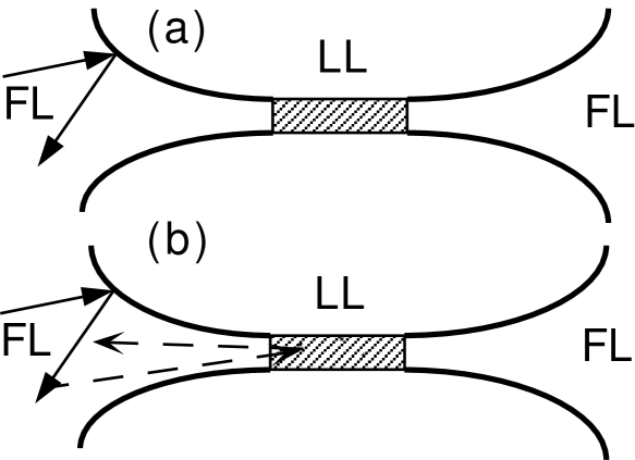
Fig. 15.: a) A Luttinger-liquid (LL) wire attached to Fermi-liquid (FL) reservoirs. b) same for a single impurity within the wire.

7.3.1 Inhomogeneous Luttinger-liquid model

An actual system consists of two Fermi-liquid reservoirs connected via a Luttinger-liquid (LL) wire and , due to the presence of the reservoirs, is not one-dimensional. In the inhomogeneous Luttinger-liquid model, the actual system is replaced by an effective 1D system, which is an infinite LL with a position-dependent interaction parameter $K(x)$ (cf. Fig. 16). The actual reservoirs are higher ($D=2$ or $3)$ systems, where the effect of the interaction can be disregarded. Consequently, the reservoirs are modelled by one-dimensional free conductors with $K_{\text{L}}=1.$ In between, $K\left(x\right)$ goes through some variation. Similarly, the charge velocity is equal to the Fermi one in the reservoirs and varies with $x$ in the middle of the system. The potential difference applied to the system produces some distribution of the electric field along the wire. The shape of this distribution is irrelevant in the dc linear response.

7.3.2 Elastic-string analogy

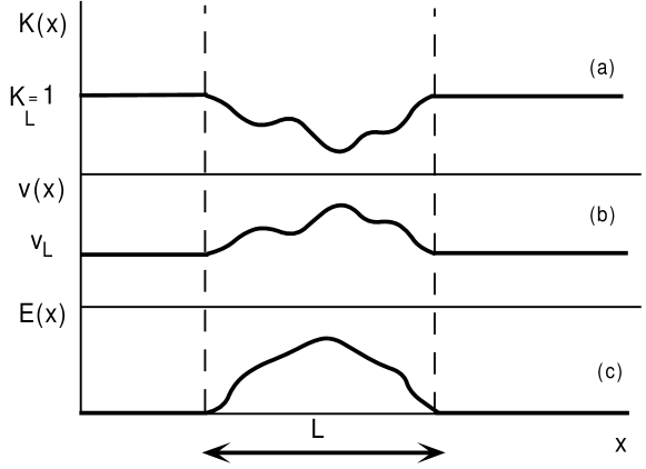
Fig. 16.: Inhomogeneous Luttinger-liquid model.

The (real-time) bosonic action for a spinless LL is

$$S=\frac{1}{2}\int d^{2}x\frac{1}{K(x)}\left\{u(x)(\partial_{x}\varphi)^{2}-\frac{1}{u(x)}(\partial_{t}\varphi)^{2}\right\}.$$ (7.13)

The density of the electrons (minus the background density) and the (number) current are given by

$$\rho=\partial_{x}\varphi/\sqrt{\pi},\qquad j=-\partial_{t}\varphi/\sqrt{\pi}.$$ (7.14)

The interaction with an external electromagnetic field $A_{\mu}$ is described by

$$S_{int}=\frac{e}{2\sqrt{\pi}}\int d^{2}x\left\{A_{0}\partial_{x}\varphi-A_{1}\partial_{t}\varphi\right\},$$ (7.15)

so that the equation of motion for $\varphi$ is

$$\partial_{t}\left(\frac{1}{Ku}\partial_{t}\varphi\right)-\partial_{x}\left(\frac{u}{K}\partial_{x}\varphi\right)=\frac{e}{\sqrt{\pi}\hbar}E(x,t),$$ (7.16)

where $E=-\partial_{x}A_{0}+\partial_{t}A_{1}$ is the electric field. We assume that the electric field is switched on at $t=0$, so that $E(x,t)=0$ for $t<0$ and $E(x,t)=E(x)$ for $t\geq 0$. The problem reduces now to determining the profile of an infinite elastic string under the external force. In this language, $\varphi(x,t)$ is the transverse displacement of the string at point $x$ and at time $t$, while the number current $j=-\partial_{t}\varphi/\sqrt{\pi}$ is proportional to the transverse velocity of the string.

To develop some intuition into the solution of Eq. (7.16), we first solve it in the homogeneous case, when $K=$const, $u=$const, and $E(x)=$const for $|x|\leq L/2,$ and is equal to zero otherwise. In this case, the solution of Eq. (7.16) for $t>L/u$, is

$$\varphi(x,t)=\frac{KeV}{2\sqrt{\pi}}\times\left\{\begin{array}[]{cl}t-\frac{x^{2}+L^{2}/4}{Lu}\;\mathrm{for}\;|x|\leq L/2;&\\ t-|x|/u\;\mathrm{for}\;L/2\leq|x|\leq ut-L/2&\\ \frac{u}{2L}\big{(}t-\frac{|x|-L/2}{u}\big{)}^{2}\;\mathrm{for}\;ut-L/2\leq|x|\leq ut+L/2\cr 0,\;\mathrm{for}\;|x|\geq ut+L/2,&\end{array}\right.$$

where $V=EL$ is the total voltage drop. This solution is depicted in Fig. 17a.

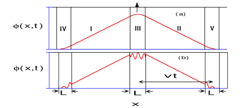
Fig. 17.: a) Solution of the wave equation in the homogeneous case for $t=5L/u$. b) Schematic solution in the inhomogeneous case for $t\gg L/u$.

The profile of the string consists of two segments (I and II in Fig. 17a) whose widths, equal to $(ut-L)$, grow with time, and of three segments (III, IV and V in Fig. 17a) whose widths are constant in time and equal to $L$. In segments I and II, the profile of the string $\varphi(x,t)$ is linear in $x$, and therefore, being the solution of the wave equation, also in $t$; in segments III-V, the profile is parabolic. Outside segments IV and V, the string is not perturbed yet, and $\varphi(x,t)=0$. As time goes on, the larger and larger part of the profile becomes linear. For late times, the pulse produced by the force spreads outwards with velocity $u$, involving the yet unperturbed parts of the string in motion; simultaneously, in all but narrow segments in the middle and at the leading edges of the pulse, the string moves upwards with the $t$- and $x$-independent “velocity” $\partial_{t}\varphi=KeV/2\sqrt{\pi}$. In terms of the original transport problem, it means that the charge current $J=-ej$ is constant outside the wire (but not too close to the edges of the regions of where the electron density is not yet perturbed by the electric field) and given by $J=Ke^{2}V/h$. Therefore, the conductance (per spin orientation) is $\mathcal{G}=Ke^{2}/h$.

We now turn to the inhomogeneous case. As in the previous case, the profile consists of several characteristic segments (cf. Fig. 17b). In segments III-V, the profile is affected by the inhomogeneities in $K(x)$, $u(x)$, and $E(x)$ and depends on the particular choice of the $x$-dependences in all these quantities. In segments I and II however, the profile, being the solution of the free wave equation, is again linear in $x$ (and in $t$). Requiring the slopes of the string be equal and opposite in segments I and II (which is consistent with the condition of the current conservation), the solution in these regions can be written as $\varphi(x,t)=A(t-|x|/u_{\mathrm{L}})$. The constant $A$ can be found by integrating Eq. (7.16) between two symmetric points $\pm a$ , chosen outside the wire

$$-\int_{-a}^{+a}dx\partial_{x}\Big{(}\frac{u}{K}\partial_{x}\varphi\Big{)}=\frac{e}{\sqrt{\pi}}\int_{-a}^{+a}dxE(x)=\frac{eV}{\sqrt{\pi}}.$$ (7.17)

Outside the wire, $K(x)=K_{\mathrm{L}}$ and $u(x)=u_{\mathrm{L}}$, thus $A=K_{\mathrm{L}}eV/2\sqrt{\pi}\hbar$. Calculating the current, we get $\mathcal{G}=K_{\mathrm{L}}e^{2}/h$ and, recalling that $K_{\mathrm{L}}=1$, we finally arrive at $\mathcal{G}=e^{2}/h$. Thus, the conductance is not renormalized by the interactions in the wire.

7.3.3 Kubo formula for a wire attached to reservoirs

The Kubo formula for a translationally non-invariant system can be written as

$$\sigma\left(\omega;x,x^{\prime}\right) = -\frac{e^{2}}{i\pi\omega}\delta\left(x-x^{\prime}\right)$$

$$+ \frac{e^{2}}{i\pi\omega}\left\{\int d\left(\tau-\tau^{\prime}\right)e^{i\omega_{m}\tau}\langle T_{\tau}\partial_{\tau}\varphi\left(x,\tau\right)\partial_{\tau^{\prime}}\varphi\left(x^{\prime},\tau^{\prime}\right)\rangle\right\}|_{i\omega_{m}\rightarrow\omega+i\delta}.$$

The diamagnetic contribution is cancelled by a delta-function term, which is obtained when integrating by parts in the time-ordered product [86, 10]. Having this in mind, I will re-write the conductivity via the Fourier transform of the $\varphi\varphi$- correlator without the $T-$ product

$$\sigma\left(\omega;x,x^{\prime}\right)=i\frac{e^{2}}{\pi\omega}\omega_{m}^{2}\Phi_{\omega_{m}}\left(x,x^{\prime}\right)|_{i\omega_{m}\rightarrow\omega+i\delta}.$$

For a translationally invariant case, this reduces back to Eq. (7.1.2). Now, $K\left(x\right)$ and $u\left(x\right)$ depend on position. The propagator of the $\varphi$ fields satisfy the wave equation (or a Laplace’s equation as we are dealing with the imaginary time)

$$\left[\frac{\omega_{m}^{2}}{u\left(x\right)K\left(x\right)}-\partial_{x}\left(\frac{u\left(x\right)}{K\left(x\right)}\partial_{x}\right)\right]\Phi_{\omega_{m}}\left(x,x^{\prime}\right)=\delta\left(x-x^{\prime}\right).$$ (7.18)

In a model of step-like variation of $K\left(x\right)$ and $u\left(x\right)$ ($K=K_{W}$ and $u=u_{W}$ within the wire and $K=K_{L}=1$ and $u=u_{L}=1$ outside the wire), Eq. (7.18) is complemented by the following boundary conditions: 1) $\Phi_{\omega_{m}}\left(x,x^{\prime}\right)$ is continuous at $x=\pm L/2,$ 2) $u\left(x\right)K\left(x\right)\partial_{x}\Phi_{\omega_{m}}\left(x,x^{\prime}\right)$ is continuous at $x=\pm L/2$; but 3) undergoes a jump of unit height at $x=x^{\prime}.$ Solution of this problem is totally equivalent to finding a potential of a point charge located somewhere in a sandwich-like system, consisting of three insulators with different dielectric constants. Two of these layers are semi-infinite and the third one (in the middle) is of finite thickness. “Potential” $\Phi_{\omega_{m}}\left(x,x^{\prime}\right)$ can be found in a general form for arbitrary $x,x^{\prime}.$ In the expression for the current

$$J\left(t,x\right)=\int dx^{\prime}\int\frac{d\omega}{2\pi}\sigma\left(\omega;x,x^{\prime}\right)E\left(\omega,x^{\prime}\right),$$

$x^{\prime}$ is within the wire; hence we need to know $\Phi_{\omega_{m}}\left(x,x^{\prime}\right)$ only for $-L/2\leq x^{\prime}\leq L/2.$ In a steady-state regime, one is free to measure the current through any cross-section; let’s choose $x$ also within the wire. As we are interested in the limit $\omega\rightarrow 0,$ when the plasmon wavelength is larger than the wire length, we can put $x=x^{\prime}.$ In the interval $-L/2<x=x^{\prime}<L/2$ the solution of the Laplace’s equation is

$$\Phi_{\omega_{m}}\left(x,x\right)=\frac{K_{W}}{2\left|\omega_{m}\right|}+\frac{K_{W}}{2\left|\omega_{m}\right|}\frac{\kappa_{-}^{2}e^{-L/L_{\omega}}+\kappa_{+}\kappa_{-}\cosh\left(2x/L_{\omega}\right)}{e^{L/L_{\omega}}\kappa_{+}^{2}-e^{-L/L_{\omega}}\kappa_{-}^{2}},$$ (7.19)

where $L_{\omega}=u_{W}/\left|\omega_{m}\right|,$ $u_{W}$ is the charge velocity within the wire, and

$$\kappa_{\pm}=K_{W}^{-1}-K_{L}^{-1}.$$

Letting $\omega_{m}$ in (7.19) to zero (and thus $L_{\omega}$ to $\infty),$ we find that

$$\Phi_{\omega}\left(x,x\right)=\frac{K_{L}}{2i\omega}=\frac{1}{2i\omega},$$

as by our assumption $K_{L}=1.$ This result is true for any $x,x^{\prime}$ within the wire for $\omega\rightarrow 0$

$$\Phi_{\omega}\left(x,x^{\prime}\right)=\frac{1}{2i\omega},\text{ for }-L/2<x,x^{\prime}<L/2.$$

The Luttinger-liquid parameters of the wire drop out from the answer. The dc conductivity reduces to its free value

$$\sigma\left(\omega\rightarrow 0;x,x^{\prime}\right)=\frac{e^{2}}{2\pi},$$

and, consequently, the conductance

$$\mathcal{G}=\frac{e^{2}}{h}$$

is not renormalized by the interaction. The same consideration for electrons with spins gives

$$\mathcal{G}=\frac{2e^{2}}{h}$$ (7.20)

7.3.4 Experiment

Most of the experiments on quantum wires indeed show that the conductance is quantizated in units of $2e^{2}/h$ at relatively high temperatures. At lower temperatures, the conductance decreases beyond the universal value and also the quantization plateaux exhibit some structure as a function of the gate voltage [90]. This can be interpreted as the effect of residual disorder: as was discussed in Secs. 5,6 transmission decreases at lower energy scales. An effect of single impurity in a quantum wire will be largely insensitive to the presence of reservoirs: as long as the transmission coefficient for an impurity is much smaller than one, the largest voltage drops occurs near the impurity rather than at the contacts to the wire. One can show that the scaling of the conductance with energy is determined by the interaction parameter $K$ inside the wire [91], in a contrast to the disorder-free case when only $K$ outside the wire matters. Also, the mesoscopic conductance fluctuations increase as the temperature goes down (the theory predicts that this effect is enhanced by the interaction [92]). As one is dealing here with a crossover regime from scattering at a single impurity to that at many impurities, a quantitative analysis of the temperature dependences is difficult; another complication arises from the finite length of the wire which cuts off scalings with temperature and voltage. In addition, at higher temperatures the first quantization plateau exhibits a well-defined step at about $0.7\times 2e^{2}/h$ [93, 94, 95, 96, 97, 98]. This “0.7” feature is not likely to result from spurious impurity scattering but rather reveals some interesting physics beyond what has been discussed so far in this review. Although the “0.7” feature deserves a review on its own, I will come back to this subject briefly in the next Section.

7.4 Spin component of the conductance

As we have shown in the previous sections, the Luttinger-liquid models predicts that conductance of a disorder-free wire is given by $e^{2}/h$ per channel at any temperature. Also, thanks to spin-charge separation, spin degrees of freedom do not play an essential role in charge transport except for giving an overall factor of two to the conductance. These two results hold as long as the Luttinger-liquid model is a good description for interacting electrons in the wire. When does this model break down? If the interaction is strong, electrons form almost a periodic 1D structure: quasi-Wigner crystal. The exchange energy of almost localized electrons is exponentially small and, correspondingly, the spin velocity is small too: $u_{s}\ll u_{c}.$ The Luttinger-liquid model should work for energies (temperatures) much smaller than the smallest of the two (spin and charge) bandwidth $T\ll u_{s}k_{F}\ll u_{c}k_{F},$ when both spin- and charge degrees of freedom are coherent. The spin- incoherent regime, i.e., $u_{s}k_{F}\ll T\ll u_{c}k_{F}$, has attracted considerable interest recently [19, 20, 21], and was shown to spoil the conductance quantization in integer multiples of $2e^{2}/h$ [19] at temperatures larger than the spin bandwidth ($u_{s}k_{F}$). In what follows, I present a short summary of Ref.[19].

In a quasi-Wigner-crystal regime, a reasonable starting point for describing the spin sector is the Heisenberg model

$$H_{s}=J_{\text{ex}}\sum_{l}\vec{S}_{l}\cdot\vec{S}_{l+1},$$

where spins are localized at “lattice sites” corresponding to positions of electrons. Because the Lieb-Mattis theorem [46] forbids ferromagnetic ordering in 1D, the sign of the exchange interaction must be antiferromagnetic: $J_{\text{ex}}>0.$ Assuming that electrons are well localized at distances $a=1/n$ from each other, $J_{\text{ex}}$ can be estimated in the WKB approximation: $J_{\text{ex}}\sim E_{F}\exp\left(-c/\sqrt{a_{B}n}\right),$ where $c\sim 1$ and $a_{B}$ is the Bohr radius. A spin-1/2 chain is then mapped onto a Hubbard 1/2-filled model of spinless fermions via the Jordan-Wigner transformation

$$S_{z}\left(l\right) = a_{l}^{\dagger}a_{l}-1/2;$$

$$S_{x}\left(l\right)+iS_{y}\left(l\right) = a_{l}^{\dagger}\exp\left(i\pi\sum_{J_{\text{ex}}=1}^{l-1}a_{J_{\text{ex}}}^{\dagger}a_{J_{\text{ex}}}\right)$$

with the result

$$H_{s}=-\frac{J_{\text{ex}}}{2}\sum\left[c_{l+1}^{\dagger}c_{l}+H.c.\right]+J_{\text{ex}}\sum:c_{l}^{\dagger}c_{l}-1/2::c_{l+1}^{\dagger}c_{l}-1/2:.$$

The spinless Hubbard model can be bosonized

$$H_{s}=\frac{1}{2}\int dx\frac{u}{K}\left(\partial_{x}\phi\right)^{2}+uK\left(\partial_{x}\theta\right)^{2}+\frac{aJ_{\text{ex}}}{\left(2\pi a\right)^{2}}\cos\left(\sqrt{16\pi}\phi\right).$$ (7.21)

A comparison to the Bethe Ansatz solution of the Hubbard model at half-filling enables one to identify the parameters of the spinless LL with the microscopic parameters of the spin-1/2 chain. In particular, for an isotropic spin chain ($J_{x}=J_{y}=J_{z}$)

$$u=\frac{\pi}{2}J_{\text{ex}}a;\;K=1/2.$$ (7.22)

Comparing the spin-part of the Hamiltonian of the original LL model, Eq. (6.29) with that of the spinless LL, Eq. (7.21), one notices that they the same upon the following mapping

$$\phi=\frac{1}{\sqrt{2}}\phi_{s};\;\text{ }\theta=\sqrt{2}\theta_{s};\;\frac{u_{s}}{K_{s}}=\frac{u}{2K};\;\text{ }u_{s}K_{s}=2uK,$$ (7.23)

or

$$u_{s}=u=\frac{\pi}{2}J_{\text{ex}}a;\;K_{s}=2K=1.$$ (7.24)

As $J_{\rm ex}$ is exponentially small, so is the spin bandwidth. Therefore, the Luttinger-liquid description is valid only at very low temperatures.

A translationally invariant LL still possesses spin-charge separation. However, this is no longer true for a wire connected to non-interacting leads. To understand this point, let’s come back to the inhomogeneous LL model (cf. Sec. 7.3.1), where the electron density changes from a higher value in the leads to a lower value within the wire. Because $J_{\text{ex}}$ depends on the local density, it is modulated along the wire, and its minimum value is at the middle of the wire. In the leads, we have a non-interacting system, where $J_{\text{ex}}\sim E_{F}\gg T.$ However, in the middle of the wire spins are incoherent, if $J_{\text{ex}}^{\min}\ll T.$ Thus a spin part of the electron incoming from the lead at energy $T$ above the Fermi level cannot propagate freely through the wire because the spin band narrows down: it works as if there is a barrier for spin excitations in the wire. Although charge plasmons propagate freely, backscattering of spin plasmons leads to additional dissipation, and thus to additional resistance. The total resistance of the wire consists now of two parts

$$R=R_{c}+R_{s}.$$

The charge part, $R_{c},$ is due to propagation of charge plasmons. Since the charge part is still described by the LL model, our previous result for universal conductance, Eq. (7.20), still holds and $R_{c}=\mathcal{G}^{-1}=h/2e^{2}.$ For $T\ll J_{\text{ex}}^{\min},$ only athermal spin plasmons, with energies exceeding the width of the spin band, contribute to $R_{s}.$ The number of such plasmons is exponentially small, hence

$$R_{s}\propto\exp\left(-J_{\text{ex}}^{\min}/T\right),$$

and total conductance $\mathcal{G=}\left(R_{c}+R_{s}\right)^{-1}$ is exponentially close to $2e^{2}/h.$ At high temperatures $\left(T\gg J_{\text{ex}}^{\min}\right)$, almost all spin plasmons are reflected by the wire. Then $R_{s}\sim R_{c}\sim h/e^{2}$, and the conductance differ substantially from its universal value. This qualitative picture can be confirmed in a particular simple case of the $XY-$ model for the spin-chain. In this case, $R_{s}$ can be calculated explicitly with the result [19]

$$R_{s}=\frac{h}{2e^{2}}\frac{1}{\exp\left(J_{\text{ex}}^{\min}/T\right)+1}$$

and, consequently, the conductance is equal to

$$\mathcal{G}=\frac{2e^{2}/h}{1+\left[\exp\left(J_{\text{ex}}^{\min}/T\right)+1\right]^{-1}}.$$

For $T\rightarrow 0,$ ${\cal G}$ approaches the universal value of $2e^{2}/h.$ For $T\gg J_{\text{ex}}^{\min}$,${\cal G}$ approaches another $T$ -independent limit, equal to $(2/3)2e^{2}/h.$ The actual number in the high-temperature limit of the conductance is model-dependent (it is different, for example, for an isotropic spin-chain), but the main result, i.e., the non-universality of conductance quantization at higher temperatures, survives.

As it was mentioned in Sec. 7.3.4, the experiment shows that there is a shoulder in the conductance preceding the first quantization plateau at a fractional value of about 0.7$\times 2e^{2}/h.$ Surprisingly, this “0.7 feature” is more pronounced at higher temperatures, and the $T$- dependence of this feature was reported to be of an activated type [95]. The magnetic field transforms the “0.7 feature” into a fully developed quantization plateau at $e^{2}/h$, which is to be expected in a fully polarized, and thus spinless, regime. The sensitivity to the magnetic field hints at the spin origin of the effect, and a significant theoretical effort was invested in understanding how spins can explain the observed phenomena. Although the effect, described in this Section, does have all qualitative characteristics of the observed “0.7 feature”, it is not clear at the moment whether this feature indeed corresponds to the spin-incoherent regime. Other explanations of the “0.7 feature” have been suggested (most prominently, the Kondo physics is believed to be involved [99, 98]), but a further discussion of this point goes beyond the scope of these notes.

7.5 Thermal conductance: Fabry-Perrot resonances of plasmons

There is an important difference between charge and thermal (electronic) conductances [22]. As we have just shown, the charge conductance is equal to $e^{2}/h$ regardless of interaction in the wire. This means that the transmission coefficient of electrons is equal to unity. The effect of the temperature on the charge conductance is the same as for a non-interacting, perfectly transmitting wire: at finite temperature, not only the lowest but also higher subbands of transverse quantization are populated, and the quantization plateaux are smeared. However, this effect is exponentially small for temperatures smaller than either the Fermi energy, $E_{F},$ or the difference between the Fermi energy and the threshold of the next subband of transverse quantization, $\Delta$; whichever is smaller.

Thermal current is carried not by electrons but bosonic excitations: acoustic plasmons. In contrast to electrons, plasmons get reflected at the boundary between the reservoirs and the wire due to the mismatch of charge velocities (this reflection happens even for an adiabatically smooth transition). From the plasmon’s point-of-view, a wire coupled to reservoirs represents a Fabry-Perrot interferometer. Interference of plasmon waves scattered off the opposite ends of the wire results in an oscillatory dependence of the transmission coefficient on the frequency with a period given by the travel time of plasmons through the wire

$$2\pi\omega_{L}=L/u_{W}.$$

As long as $\lambda_{F}\ll L,$ this period is long: $\omega_{L}\ll E_{F}$ . The difference between charge and heat transport is that the chemical potential of plasmons is equal to zero, and thus the characteristic scale for frequency is set by $T$. Therefore, the thermal conductance varies with the temperature on a scale $T\simeq\omega_{L}.$

Suppose that a small temperature difference $\delta T$ is maintained between the reservoirs, connected by a quantum wire. As the Hamiltonian of an interacting system is diagonalized of terms of plasmons, plasmons modes are decoupled and contribute to the energy flux independently. Then the thermally averaged energy current, i.e., the thermal current can be found via a Landauer-like argument

$$J_{T}=\int_{0}^{\infty}\frac{d\omega}{2\pi}\omega\left|t\left(\omega\right)\right|^{2}\left(n_{L}\left(\frac{\omega}{T+\delta T}\right)-n_{R}\left(\frac{\omega}{T}\right)\right),$$

where $n_{L,R}\left(\omega/T\right)$ are the Bose distribution functions in the reservoirs. Expanding in small $\delta T,$ we obtain the thermal conductance

$$\mathcal{G}_{T}=\frac{J_{T}}{\delta T}=\frac{1}{8\pi T^{2}}\int_{0}^{\infty}d\omega\frac{\omega^{2}}{\sinh^{2}\omega/2T}\left|t\left(\omega\right)\right|^{2}.$$ (7.25)

For a free system, $\left|t\left(\omega\right)\right|^{2}=1$ and $\mathcal{G}_{T}=\pi T/6.$ The charge and thermal conductances of a free system obey the Wiedemann-Franz law

$$\frac{\mathcal{G}_{T}}{T\mathcal{G}}=L_{0}=\frac{\pi^{2}}{3e^{2}},$$ (7.26)

where $L_{0}$ is the Lorentz number. This means that charge and energy are carried by the same excitations. This is not so in a Luttinger liquid.

For an interacting system, relation (7.26) holds in the limit of $T\rightarrow 0.$ The characteristic scale for frequencies in integral (7.25) is determined by $T.$ For $T\ll\omega_{L}$, one can substitute $\omega=0$ into $\left|t\left(\omega\right)\right|^{2}.$ Regardless of the interaction strength, $\left|t\left(0\right)\right|^{2}=1:$ a Fabry-Perrot interferometer becomes transparent in the long wavelength limit. For $T\gtrsim\omega_{L},$ the result for $\mathcal{G}_{T}$ depends on how the charge velocity varies along the wire, and is thus non-universal. On the other hand, the charge conductance is universal. Therefore, their ratio is non-universal and the Wiedemann-Franz law is violated.

In a step-like model of Sec. 7.3.1, the transmission coefficient of plasmons is equal to

$$\left|t\left(\omega\right)\right|^{2}=\frac{1}{1+\frac{\left(K^{2}-1\right)^{2}}{4K^{2}}\sin^{2}\frac{\omega}{\omega_{L}}}.$$

Obviously, $\left|t\left(0\right)\right|^{2}=1$ regardless of $K,$ an agreement with what was said above. For $T\ll\omega_{L},$ the Lorentz number is close to the universal value of $\pi^{2}/3e^{2}.$ For $T\gg\omega_{L}$, the oscillations of $\left|t\left(\omega\right)\right|^{2}$ become very fast, so that $\left|t\left(\omega\right)\right|^{2}$ can be replaced by its averaged value

$$\langle\left|t\left(\omega\right)\right|^{2}\rangle=\int_{0}^{\omega_{L}}\frac{d\omega}{\omega_{L}}\left|t\left(\omega\right)\right|^{2}=\frac{2K}{K^{2}+1}.$$

The thermal conductance increases linearly with $T,$ so that $L_{0}$ approaches a constant but a non-universal value

$$L|_{T\gg\omega_{L}}=\frac{2K}{K^{2}+1}L_{0}<L_{0}.$$ (7.27)

As the Lorentz number varies with temperature in between two limits specified by Eqs.(7.26) and (7.27), the Wiedemann-Franz law is violated.

8 Acknowledgments

Late R. Landauer and H. J. Schulz helped me–either directly or indirectly, through their writings–to form my way of thinking about interactions and transport, and my gratitude goes to their memories. I benefited tremendously from discussions with B. L. Altshuler, C. Biagini, C. Pèpin, A. V. Chubukov, V. V. Cheianov, E. Fradkin, F. Essler, S. Gangadharaiah, Y. Gefen, L. I. Glazman, P. M. Goldbart, I. V. Gornyi, Y. B. Levinson, D. Loss, K. A. Matveev, B. N. Narozhny, A. A. Nersesyan, D. G. Polyakov, C. Pépin, M. Yu. Reizer, I. Safi, R. Saha, B. I. Shklovskii, M. Stone, O. A. Starykh, S. Tarucha, S.-W. Tsai, A. Yacoby, O. M. Yevtushenko, and M. B. Zvonarev on various subjects discussed in these notes. I am also grateful to the organizers of the 2004 Summer School in Les Houches–H. Bouchiat, Y. Gefen, S. Guéron, and G. Montambaux–for assembling a very interesting program and providing a stimulating environment, as well as to the all participants of the School for their questions, attention, and patience. S. Gangadharaiah, L. Merrill, and R. Saha kindly helped me with producing the images. S. Gangadharaiah, P. Kumar, C. Pépin, R. Saha, and S.-W. Tsai proofread parts of the manuscript (which does not make them responsible for the typos). I acknowledge the hospitality of the Abdus Salam International Centre for Theoretical Physics (Trieste, Italy), where a part of this manuscript was written. Financial support from NSF DMR-0308377 is greatly appreciated.

Appendix A Polarization bubble for small $q$ in arbitrary dimensionality

The polarization bubble in Matsubara frequencies and at $T=0$ is given by

$$\Pi\left(i\omega,q\right) = \frac{N_{s}}{\left(2\pi\right)^{D+1}}\int\int d^{D}pd\varepsilon G\left(i\varepsilon+i\omega,\vec{p}+\vec{q}\right)G\left(i\varepsilon,p\right)$$

$$= \frac{N_{s}}{\left(2\pi\right)^{D+1}}\int\int d^{D}pd\varepsilon\frac{1}{i\omega-\xi_{\vec{p}+\vec{q}}+\xi_{\vec{p}}}\left[G\left(i\varepsilon+i\omega,\vec{p}+\vec{q}\right)-G\left(i\varepsilon,p\right)\right]$$

$$= \frac{N_{s}}{\left(2\pi\right)^{D+1}}\int d^{D}p\frac{f\left(|\vec{p}+\vec{q}|\right)-f\left(p\right)}{i\omega-\xi_{\vec{p}+\vec{q}}+\xi_{\vec{p}}},$$

where $f$ is the Fermi function. Expanding in $\vec{q},$ and switching from the integration over $d^{D}p$ to $d\xi,$ we obtain

$$\Pi\left(i\omega,q\right)=-N_{s}\nu_{D}\left(1-\int\frac{d\Omega}{\Omega_{D}}\frac{i\omega}{i\omega-v_{F}q\cos\theta}\right).$$

where $\Omega_{D}=4\pi$ (3D), $=2\pi\left(2D\right),$ $=2$ (1D) and $\nu_{D}$ is the DoS in $D$ dimensions per one of the $N_{s}$ isospin components. For D=1, the integral over $\Omega$ is understood as a sum of terms with $\cos\theta=\pm 1.$ It is obvious already this form that the small $q-$form of the bubble depends on the combination $\omega/v_{F}q$ for any $D.$ The final result depends on the dimensionality. Performing analytic continuation to real frequencies $i\omega\rightarrow\omega+i0^{+},$ we obtain

$$\Pi^{R}\left(\omega,q\right)=-N_{s}\nu_{D}\left(1-\int\frac{d\Omega}{\Omega_{D}}\frac{\omega}{\omega-v_{F}q\cos\theta+i0}\right).$$

Taking the imaginary part

$$\mathrm{Im}\Pi^{R}\left(\omega,q\right)=-\pi N_{s}\nu_{D}\omega\int\frac{d\Omega}{\Omega_{D}}\delta\left(\omega-v_{F}q\cos\theta\right).$$ (A. 1)

From here

$$\cos\theta=\omega/v_{F}q,$$

which means that $\theta\approx\pi/2$ for $\omega\ll v_{F}q.$ Thus, the fermionic momentum $\vec{p}$ is almost perpendicular to the bosonic one, $\vec{q},$ in this limit.

Appendix B Polarization bubble in 1D

Appendix B.1 Small $q$

Free time-ordered (causal) Green’s function in 1D is equal to

$$G_{\pm}^{0}\left(\varepsilon,k\right)=\frac{1}{\varepsilon-\xi_{k}^{\pm}+i0^{+}\mathrm{sgn}\xi_{k}^{\pm}},$$

where

$$\xi_{k}^{\pm}=\pm v_{F}\left(k\mp k_{F}\right),$$

and $\pm$ signs correspond to right/left moving fermions. We will be measuring the momenta from the corresponding Fermi points. For +branch :$k-k_{F}\rightarrow k$ and for -branch: $k+k_{F}\rightarrow k.$ Consequently,

$$G_{\pm}^{0}\left(\varepsilon,k\right)=\frac{1}{\varepsilon\mp v_{F}k+i0^{+}\mathrm{sgn}k}.$$

I assume the $N_{s}-$ fold degeneracy ($N_{s}=2$ for electrons with spin, $N_{s}=1$ for spinless electrons), so that

$$\Pi_{\pm}\left(\omega,q\right)=-\frac{i}{\left(2\pi\right)^{2}}N_{s}\int d\varepsilon\int dkG_{\pm}^{0}\left(\varepsilon+\omega,k+q\right)G_{\pm}^{0}\left(\varepsilon,k\right).$$

Calculate, e.g., $\Pi_{+}:$

$$\Pi_{+}\left(\omega,q\right) = -\frac{i}{\left(2\pi\right)^{2}}N_{s}\int d\varepsilon\int dk\frac{1}{\varepsilon+\omega-v_{F}(k+q)+i0^{+}\mathrm{sgn(}k+q)}\frac{1}{\varepsilon-v_{F}k+i0^{+}\mathrm{sgn}k}$$ (B. 2)

$$= -\frac{i}{\left(2\pi\right)^{2}}N_{s}\int d\varepsilon\int dk\frac{1}{\omega-v_{F}q+i0^{+}\mathrm{sgn(}k+q)-i0^{+}\mathrm{sgn}k}$$

$$\times\left[G_{+}^{0}\left(\varepsilon,k\right)-G_{+}^{0}\left(\varepsilon+\omega,k+q\right)\right].$$

The integral of the Green’s over the frequency gives a Fermi distribution function [23]

$$n_{+}\left(k\right)=-i\int\frac{d\varepsilon}{2\pi}G_{+}^{0}\left(\varepsilon,k\right).$$

For free fermions,

$$n_{+}\left(k\right)=\theta\left(-k\right)$$

Now,

$$\Pi_{+}^{0}\left(\omega,q\right)=\frac{N_{s}}{2\pi}\int dk\frac{1}{\omega-v_{F}q+i0^{+}\mathrm{sgn(}k+q)-i0^{+}\mathrm{sgn}k}\left[\theta\left(-k\right)-\theta\left(-k-q\right)\right].$$

The integral is not equal to zero only if the arguments of the $\theta$ -functions are of the opposite signs. Consider different situations.

1) $k>0$; $k+q<0\rightarrow 0<k<-q\rightarrow q<0.$ In this case,

$$\Pi_{+}^{0}\left(\omega,q\right)=\frac{N_{s}}{2\pi}\frac{q}{\omega-v_{F}q-i0^{+}},\mathrm{\ }q<0;$$

2) $k<0,$ $k+q>0\rightarrow-q<k<0\rightarrow q>0$

$$\Pi_{+}^{0}\left(\omega,q\right)=\frac{N_{s}}{2\pi}\frac{q}{\omega-v_{F}q+i0^{+}},q>0.$$

Combining the results for $q>0$ and $q<0$ together,

$$\Pi_{+}^{0}\left(\omega,q\right)=\frac{N_{s}}{2\pi}\frac{q}{\omega-v_{F}q+i0^{+}\mathrm{sgn}q}.$$ (B. 3)

Similarly,

$$\Pi_{-}^{0}\left(\omega,q\right)=-\frac{N_{s}}{2\pi}\frac{q}{\omega-v_{F}q+i0^{+}\mathrm{sgn}\omega}.$$ (B. 4)

The total bubble

$$\Pi^{0}\left(\omega,q\right)=\Pi_{+}^{0}\left(\omega,q\right)+\Pi_{-}^{0}\left(\omega,q\right)=\frac{N_{s}}{\pi}\frac{v_{F}q^{2}}{\omega^{2}-v_{F}^{2}q^{2}+i0^{+}}.$$ (B. 5)

In what follows, we will also need the retarded and advanced form of the bubble. These forms can easily be obtained by repeating the calculation above in Matsubara frequencies and analytically continuing $i\omega_{m}\rightarrow\omega+i0$ . Even simpler, one can use the general relation between time-ordered and retarded propagators [23] (which works equally well for fermionic and bosonic quantities)

$$\Pi_{\pm}^{R}\left(\omega,q\right) = \Pi_{\pm}\left(\omega,q\right),\text{ }\mathrm{for}\text{ }\mathrm{\omega>0}$$

$$= \Pi_{\pm}^{\ast}\left(\omega,q\right),\text{ }\mathrm{for}\text{ }\mathrm{\omega<0.}$$

Using Eqs. (B. 3) and (B. 4) we obtain

$$\Pi_{\pm}^{R}\left(\omega,q\right)=\pm\frac{N_{s}}{2\pi}\frac{q}{\omega-v_{F}q+i0^{+}}$$ (B. 6)

and

$$\Pi^{R}\left(\omega,q\right) = \frac{N_{s}}{\pi}\frac{v_{F}q^{2}}{\omega^{2}-v_{F}^{2}q^{2}+i0^{+}sgn\omega}$$ (B. 7)

$$= \frac{N_{s}}{\pi}\frac{v_{F}q^{2}}{\left(\omega+i0^{+}\right)^{2}-v_{F}^{2}q^{2}}.$$

Appendix B.2 $q$ near $2k_{F}$

We will also need the $2k_{F}$ bubble. This time, I choose to do the calculation in Matsubara frequencies:

$$\Pi_{2k_{F}}\left(i\omega,q\right) = \frac{N_{s}}{(2\pi)^{2}}\int dk\int d\varepsilon G_{+}\left(i\varepsilon+i\omega,k+q\right)G_{-}\left(i\varepsilon,k\right)$$

$$= -\frac{N_{s}}{(2\pi)^{2}}\int dk\int d\varepsilon\frac{1}{\varepsilon+\omega+i\left(k+q\right)}\frac{1}{\varepsilon-ik}.$$

Poles in $\varepsilon_{1}=ik$ and $\varepsilon_{2}=-i\left(k+q\right)-\omega$ have to be on different sides of the real axis, otherwise the integral is equal to zero. Choose $q>0.$ Then this condition is satisfied in two intervals of $k:$ $k>0$ and $-\Lambda/2<k<-q,$ where $\Lambda$ is the ultraviolet cut-off

$$\Pi_{2k_{F}} = -\frac{iN_{s}}{2\pi}\left[\int_{0}^{\Lambda/2}dk-\int_{-\Lambda/2}^{-q}dk\right]\frac{1}{\omega+2iv_{F}k+iv_{F}q}$$ (B. 8)

$$= -\frac{N_{s}}{4\pi}\left[\ln\frac{i\Lambda v_{F}}{\omega+iv_{F}q}-\ln\frac{\omega-iv_{F}q}{-i\Lambda v_{F}}\right]$$

$$= -\frac{N_{s}}{4\pi}\ln\frac{\Lambda^{2}v_{F}^{2}}{\omega^{2}+v_{F}q^{2}}.$$

Because the result depends on $q^{2}$ there is no need for a separate calculation for the case $q<0.$

Appendix C Some details of bosonization procedure

Appendix C.1 Anomalous commutators

$$\rho\left(q\right) = \sum_{p}a_{p-q/2}^{\dagger}a_{p+q/2}=\rho_{+}+\rho_{-};$$

$$\rho_{\pm} = \sum_{p>0(p<0)}a_{p-q/2}^{\dagger}a_{p+q/2}.$$

The operators of full density commute. The operators of left-right densities have non-trivial commutators. For example, let us calculate $\left[\rho_{+}\left(q\right),\rho_{+}\left(q^{\prime}\right)\right]$

$$C_{++}\left(q,q^{\prime}\right) = \left[\rho_{+}\left(q\right),\rho_{+}\left(q^{\prime}\right)\right]=\sum_{p>0,k>0}\left[a_{p-q/2}^{\dagger}a_{p+q/2},a_{k-q^{\prime}/2}^{\dagger}a_{k+q^{\prime}/2}\right]$$

$$= \sum_{p>0,k>0}\left(\begin{array}[]{c}a_{p-q/2}^{\dagger}\underbrace{a_{p+q/2}a_{k-q^{\prime}/2}^{\dagger}}_{=\delta_{p+q/2,k-q^{\prime}/2}-a_{k-q^{\prime}/2}^{\dagger}a_{p+q/2}}a_{k+q^{\prime}/2}\\ -a_{k-q^{\prime}/2}^{\dagger}\underbrace{a_{k+q^{\prime}/2}a_{p-q/2}^{\dagger}}_{=\delta_{k+q^{\prime}/2,p-q/2}-a_{p-q/2}^{\dagger}a_{k+q^{\prime}/2}}a_{p+q/2}\end{array}\right).$$

The first $\delta-$ function means that $k=p+q/2+q^{\prime}/2>0$ and the second one that $k=p-q/2-q^{\prime}/2.$

$$C_{++}\left(q,q^{\prime}\right) = \sum_{p>0}a_{p-q/2}^{\dagger}a_{p+q/2+q^{\prime}}\vartheta\left(p+q/2+q^{\prime}/2\right)-a_{p-q/2-q^{\prime}}^{\dagger}a_{p+q/2}\theta\left(p-q/2-q^{\prime}/2\right)$$

$$-\left[f\left(q,q^{\prime}\right)-f\left(q^{\prime},q\right)\right],$$

where

$$f(q,q^{\prime}) = \sum_{p,k>0}a_{p-q/2}^{\dagger}a_{k-q^{\prime}/2}^{\dagger}a_{p+q/2}a_{k+q^{\prime}/2}$$

$$= \sum_{p,k>0}a_{p}^{\dagger}a_{k}^{\dagger}a_{p+q}a_{k+q^{\prime}}$$

It is easy to show that $f\left(q,q^{\prime}\right)=f\left(q^{\prime},q\right).$ Indeed,

$$f(q^{\prime},q) = \sum_{p,k>0}a_{p}^{\dagger}a_{k}^{\dagger}a_{p-q^{\prime}}a_{k+q}$$

$$= \underset{}{\mathrm{re-labelling}\text{ }\mathrm{k\longleftrightarrow p=}}\sum_{p,k>0}a_{k}^{\dagger}a_{p}^{\dagger}a_{k-q^{\prime}}a_{p+q}$$

$$= \underset{}{\mathrm{{anticommuting}=}}\sum_{p,k>0}a_{p}^{\dagger}a_{k}^{\dagger}a_{p+q}a_{k+q^{\prime}}=f\left(q,q^{\prime}\right).$$

Thus

$$C_{++}\left(q,q^{\prime}\right)=\sum_{p>0}a_{p-q/2}^{\dagger}a_{p+q/2+q^{\prime}}\theta\left(p+q/2+q^{\prime}/2\right)-a_{p-q/2-q^{\prime}}^{\dagger}a_{p+q/2}\theta\left(p-q/2-q^{\prime}/2\right).$$

Introduce a new momentum

$$Q=\frac{q+q^{\prime}}{2}.$$

In the first sum, shift $p+q^{\prime}/2\rightarrow p$ and in the second sum shift $p-q^{\prime}/2\rightarrow p.$ Then

$$C_{++}\left(q,2Q-q\right) = \sum_{p>0}a_{p-Q}^{\dagger}a_{p+Q}\left[\theta\left(p+q/2\right)-\theta\left(p-q/2\right)\right]$$

$$= \sum_{p>-q/2}a_{p-Q}^{\dagger}a_{p+Q}-\sum_{p>q/2}a_{p-Q}^{\dagger}a_{p+Q}$$

If the main contribution to the sum is given by the states which lie either deep below or far above the Fermi levels, then the quantum fluctuations in the occupancy of these states are small, and the operators $a_{p-Q}^{\dagger}a_{p+Q}$ can be replaced by their expectation values $\langle a_{\pi-Q}^{\dagger}a_{p+Q}\rangle=\delta_{Q,0}n_{p}=$ $\delta_{Q,0}\theta\left(p_{F}-p\right)$. Doing this, we find

$$C_{++}\left(q,2Q-q\right) = \delta_{Q,0}\left(\sum_{p>-q/2}^{p_{F}}-\sum_{p>q/2}^{p_{F}}\right)=\delta_{Q,0}\frac{L}{2\pi}\left(\int_{-q/2}^{p_{F}}dp-\int_{q/2}^{p_{F}}dp\right)$$

$$= \delta_{Q,0}\frac{qL}{2\pi}.$$

Therefore,

$$[\rho_{+}\left(q),\rho_{+}(-q\right)]=\frac{qL}{2\pi},\mathrm{spinless.}$$ (C. 2)

The same procedure for fermions with spin gives

$$[\rho_{+,\sigma}\left(q),\rho_{+,\sigma^{\prime}}(-q\right)]=\delta_{\sigma\sigma^{\prime}}\frac{qL}{2\pi},\mathrm{with}\text{ }\mathrm{spin.}$$

Similarly,

$$[\rho_{-,\sigma}\left(q),\rho_{-,\sigma^{\prime}}(-q\right)]=-\delta_{\sigma\sigma^{\prime}}\frac{qL}{2\pi},\mathrm{with}\text{ }\mathrm{spin.}$$

and

$$[\rho_{+,\sigma}\left(q),\rho_{-,\sigma}(-q\right)]=0.$$

Combining these results together

$$\left[\rho_{\alpha,\sigma}\left(q\right),\rho_{\alpha^{\prime},\sigma^{\prime}}\left(-q\right)\right]=\alpha\delta_{\alpha,\alpha^{\prime}}\delta_{\sigma,\sigma^{\prime}}\frac{qL}{2\pi},$$

where $\alpha=\pm$ is the chirality index. For full charge density and current, it means that

$$\left[\rho^{c}\left(q\right),\rho^{c}\left(-q\right)\right] = \left[\rho_{+}^{c}\left(q\right)+\rho_{-}^{c}\left(q\right),\rho_{+}^{c}\left(-q\right)+\rho_{-}^{c}\left(-q\right)\right]$$

$$= \frac{qV}{2\pi}+\frac{qV}{2\pi}-\frac{qV}{2\pi}-\frac{qV}{2\pi}=0.$$

Similarly,

$$\left[j^{c}\left(q\right),j^{c}\left(-q\right)\right]=0,$$

whereas

$$\left[\rho^{c}\left(q\right),j^{c}\left(-q\right)\right]=\frac{qV}{2\pi}{\small+}\frac{qV}{2\pi}{\small+}\frac{qV}{2\pi}{\small+}\frac{qV}{2\pi}{\small=}\frac{2}{\pi}qL.$$

In 4-notations,

$$[j^{\mu}\left(q\right),j^{\nu}\left(-q\right)]=\epsilon^{\mu\nu}\frac{2}{\pi}qL,$$

where $\epsilon^{00}=\epsilon^{11}=0,$ $\epsilon^{01}=-\epsilon^{10}=1.$

Appendix C.2 Bosonic operators

Let’s check that the representation of density operators via standard bosonic operators does reproduce commutation relation for density. Expand the density operators over the normal modes

$$\rho_{+}\left(x\right) = \frac{1}{L}\sum_{q>0}A_{q}\left(b_{q}e^{iqx}+b_{q}^{\dagger}e^{-iqx}\right);$$

$$\rho_{-}\left(x\right) = \frac{1}{L}\sum_{q<0}A_{q}\left(b_{q}e^{iqx}+b_{q}^{\dagger}e^{-iqx}\right),$$

where, without a loss of generality, $A_{q}$ can be chosen real and even function of $q.$ Fourier transforming $\rho_{+}\left(x\right)$

$$\rho_{+}\left(q\right) = \int_{-\infty}^{\infty}dxe^{-iqx}\frac{1}{L}\sum_{q^{\prime}>0}A_{q^{\prime}}\left(b_{q^{\prime}}e^{iq^{\prime}x}+b_{q^{\prime}}^{\dagger}e^{-iq^{\prime}x}\right),$$

$$= A_{q}\left(\theta\left(q\right)b_{q}+\theta\left(-q\right)b_{-q}^{\dagger}\right).$$

Choose $q>0$ and substitute (Appendix C.2) into the commutation relation

$$\left[\rho_{+}\left(q\right),\rho_{+}\left(-q\right)\right] = A_{q}^{2}\left[b_{q},b_{q}^{\dagger}\right]=A_{q}^{2}=\frac{qL}{2\pi}\rightarrow$$

$$A_{q} = \sqrt{\frac{qL}{2\pi}}.$$

Appendix C.2.1 Commutation relations for bosonic fields $\varphi$ and $\vartheta$

Using

$$\varphi\left(x\right) = -i\sum_{-\infty<q<\infty}\frac{1}{\sqrt{2\left|q\right|L}}{\rm sgn}q\left(b_{q}e^{iqx}-b_{q}^{\dagger}e^{-iqx}\right);$$

$$\vartheta\left(x\right) = i\sum_{-\infty<q<\infty}\frac{1}{\sqrt{2\left|q\right|L}}\left(e^{iqx}b_{q}-b_{q}^{\dagger}e^{-iqx}\right);$$

$$\vartheta^{\prime}\left(x\right) = -\sum_{-\infty<q<\infty}\frac{1}{\sqrt{2\left|q\right|L}}q\left(e^{iqx}b_{q}+b_{q}^{\dagger}e^{-iqx}\right),$$

we find

$$\left[\varphi\left(x\right),\vartheta^{\prime}\left(x\right)\right] = i\sum_{q,q^{\prime}}\frac{1}{\sqrt{2\left|q\right|L}}\frac{1}{\sqrt{2\left|q\right|^{\prime}L}}\left|q^{\prime}\right|$$

$$\times\underbrace{\left[b_{q}e^{iqx}-b_{q}^{\dagger}e^{-iqx},b_{q^{\prime}}e^{iq^{\prime}x^{\prime}}-b_{q^{\prime}}^{\dagger}e^{iq^{\prime}x^{\prime}}\right]}_{=2\delta_{q,-q^{\prime}}}$$

$$= i\frac{1}{L}\sum_{q}e^{iq\left(x-x^{\prime}\right)}=i\delta\left(x-x^{\prime}\right).$$

Appendix C.3 Problem with backscattering

As it was pointed out in the main text, straightforward bosonization of the Hamiltonian for the spinless case encounters a problem if one tries to account for backscattering. As backscattering ($g_{1}$) is just an exchange process to forward scattering of fermions of opposite chiralities ($g_{2}$), the Luttinger liquid parameters with $g_{1}\neq 0$ should be obtained from those with $g_{1}=0$ by a simple replacement: $g_{2}\rightarrow g_{2}-g_{1}.$ However, if we do this, we cannot satisfy the Pauli principle which says that for a contact interaction, when $g_{2}=g_{4}=g_{1}$, all the interaction effects should disappear. Indeed, Eqs.6.2) and (6.11) for $u$ and $K$, correspondingly, change to

$$u^{2} = \left(1+\frac{g_{4}}{2\pi}\right)^{2}-\left(\frac{g_{2}-g_{1}}{2\pi}\right)^{2};$$

$$K^{2} = \frac{1+\frac{g_{4}-g_{2}+g_{1}}{2\pi}}{1+\frac{g_{4}+g_{2}-g_{1}}{2\pi}}.$$

For contact interaction, when $g_{2}=g_{4}=g_{1},$ we get

$$u^{2} = \left(1+\frac{g}{2\pi}\right)^{2}\neq 1$$

$$K = 1.$$

The charge velocity is different from 1. In addition, the product $uK$ is renormalized from unity–this is also a problem, as it means that the current operator is renormalized by the interactions. How to fix this problem? Ref. [77] shows how to arrive at the expressions for $u$ and $K$ which satisfy all necessary constraints just on the basis on Galilean invariance and dimensional analysis. Ref. [78] arrives at the same result by using a careful point-splitting of the operators. Here, I present the method of Ref. [78].

Recall that the density operator, represented in terms of bosonic fields, contains not only the lowest harmonic ($q\rightarrow 0$), corresponding to long-wavelength excitations, but also harmonics oscillating at $q=2k_{F},$ $4k_{F},$ etc. Indeed, taking into account only the $2k_{F}-$ oscillations, we have

$$\rho\left(x\right) = \left(\psi_{+}^{\dagger}\left(x\right)e^{-ik_{F}x}+\psi_{-}^{\dagger}\left(x\right)e^{ik_{F}x}\right)\left(\psi_{+}\left(x\right)e^{ik_{F}x}+\psi_{-}\left(x\right)e^{-ik_{F}x}\right)$$

$$= \psi_{+}^{\dagger}\left(x\right)\psi_{+}\left(x\right)+\psi_{-}^{\dagger}\left(x\right)\psi_{-}\left(x\right)+e^{-2ik_{F}x}\psi_{+}^{\dagger}\left(x\right)\psi_{-}\left(x\right)+H.c.$$

The first term in this equation has to be treated using the point-splitting procedure, because it involves two fermionic operators at the same point. The result is an infinite constant, $\rho_{0},$ which is just a uniform density, plus the gradient term. The $2k_{F}$ -component can be bosonized without a problem, as it involves products of different fermions. The result is

$$\rho\left(x\right)-\rho_{0}=\frac{1}{\sqrt{\pi}}\partial_{x}\varphi+\frac{1}{2\pi\alpha}\exp\left[2\sqrt{\pi}\varphi+2k_{F}x\right]+H.c.$$

Using this expression for the interaction part of $H,$ we have

$$H_{\text{int}} = \frac{1}{2}\int dx\int dx^{\prime}V\left(x-x^{\prime}\right)\left[\rho\left(x\right)-\rho_{0}\right]\left[\rho\left(x^{\prime}\right)-\rho_{0}\right]$$

$$= H_{F}+H_{B},$$

where the forward and backscattering parts of the Hamiltonian are given by

$$H_{F} = \frac{1}{2\pi}\int dx\int dx^{\prime}V\left(x-x^{\prime}\right)\partial_{x}\varphi\partial_{x^{\prime}}\varphi;$$

$$H_{B} = \frac{1}{2}\left(\frac{1}{2\pi a}\right)^{2}\int dx\int dx^{\prime}V\left(x-x^{\prime}\right)$$

$$\times\left\{\exp\left[2i\sqrt{\pi}\varphi\left(x\right)\right]\exp\left[-2i\sqrt{\pi}\varphi\left(x^{\prime}\right)\right]e^{2ik_{F}\left(x-x^{\prime}\right)}+H.c\right\}.$$

In $H_{B}$, we neglected the terms that oscillate with $x,x^{\prime},$and $x+x^{\prime}$, and kept only those terms that oscillate with $x-x^{\prime}.$ As our potential is sufficiently short-ranged, the oscillations of the first group of terms will average out, whereas the second group will survive. Introducing new coordinates

$$R \equiv \frac{x+x^{\prime}}{2};$$

$$r \equiv x-x^{\prime},$$

and assuming that $\left|R\right|\gg\left|r\right|,$ the forward-scattering part of the Hamiltonian reduces to

$$H_{F}=\frac{1}{2\pi}\int dR\left(\partial_{R}\varphi\right)^{2}\int drV\left(r\right)=\frac{V(0)}{2\pi}\int dR\left(\partial_{R}\varphi\right)^{2}.$$

The product of the two exponentials needs to be evaluated with care. Applying the Baker-Hausdorff identity

$$e^{A}e^{B}=:e^{A+B}:e^{\langle AB-\frac{1}{2}A^{2}-\frac{1}{2}B^{2}\rangle},$$

we get

$$\exp\left[2i\sqrt{\pi}\varphi\left(x\right)\right]\exp\left[-2i\sqrt{\pi}\varphi\left(x^{\prime}\right)\right] = \exp\left[2i\sqrt{\pi}\left(\varphi\left(x\right)-\varphi\left(x^{\prime}\right)\right)\right]:$$

$$\times\exp[4\pi\langle\varphi\left(x-x^{\prime}\right)\varphi\left(0\right)-\varphi^{2}\left(0\right)],$$

Using the expression for the free bosonic propagator

$$\langle\varphi\left(x-x^{\prime}\right)\varphi\left(0\right)-\varphi^{2}\left(0\right)]=\frac{1}{4\pi}\ln\frac{a^{2}}{(x-x^{\prime})^{2}},$$

and expanding in $r=x-x^{\prime}$ under the normal-ordering sign, we obtain

$$\exp\left[2i\sqrt{\pi}\varphi\left(x\right)\right]\exp\left[-2i\sqrt{\pi}\varphi\left(x^{\prime}\right)\right]=-\frac{1}{2}4\pi\left(\partial_{R}\varphi\right)^{2}r^{2}\frac{a^{2}}{r^{2}}=-2\pi\left(\partial_{R}\varphi\right)^{2}a^{2}.$$

(While expanding, we neglected the first derivative of $\varphi$ which can be always eliminated by choosing appropriate boundary condition.). $H_{B}$ reduces to

$$H_{B} = -\frac{1}{2}\left(\frac{1}{2\pi a}\right)^{2}2\pi a^{2}\int dR\left(\partial_{R}\varphi\right)^{2}\int drV\left(r\right)2\cos 2k_{F}r$$

$$= -\frac{1}{2\pi}\int dR\left(\partial_{R}\varphi\right)^{2}\int drV\left(r\right)\cos 2k_{F}r$$

$$= -\frac{V\left(2k_{F}\right)}{2\pi}\int dR\left(\partial_{R}\varphi\right)^{2}.$$

Therefore, the bosonized form of the total Hamiltonian

$$H_{int}=\frac{V\left(0\right)-V\left(2k_{F}\right)}{2\pi}\int dR\left(\partial_{R}\varphi\right)^{2}$$

manifestly obeys the Pauli principle. The Luttinger-liquid parameters are now given by

$$u=\sqrt{1+\frac{V\left(0\right)-V\left(2k_{F}\right)}{2\pi}};\;K=\frac{1}{\sqrt{1+\frac{V\left(0\right)-V\left(2k_{F}\right)}{2\pi}}}.$$

References

- [1] J. Solóyom, Adv. Phys. 28, 209 (1979).
- [2] V. J. Emery, in Highly Conducting One-Dimensional Solids, eds. J. T. Devreese, R. E. Evrard, and V. E. van Doren, (Plenum Press, New York, 1979), p. 247.
- [3] H. J. Schulz, in Mesoscopic Quantum Physics, Les Houches XXI (eds. E. Akkermans, G. Montambaux, J. L. Pichard, and J. Zinn-Justin), (Elsevier, Amsterdam, 1995), p. 533.
- [4] R. Shankar, Rev. Mod. Phys. 66, 129 (1994).
- [5] J. Voit, Rep. Prog. Phys. 58, 977 (1995).
- [6] A. M. Tsvelik, Quantum Field Theory in Condensed Matter Physics, (Cambridge, 1995).
- [7] M. P. A. Fisher and L. I. Glazman, in Mesoscopic Electron Transport, ed. L. Kouwenhoven et al. (Kluwer, Dordrecht); cond-mat/9610037.
- [8] J. von Delft, H. Schoeller, Ann. Phys. 7, 225 (1998).
- [9] A. O. Gogolin, A. A. Nersesyan, ad A. M. Tsvelik, Bozonization and Strongly Correlated Systems (Cambridge, 1998).
- [10] T. Giamarchi, Quantum Physics in One Dimension (Oxford, 2004)
- [11] K. A. Matveev, D. Yue, and L. I. Glazman, Phys. Rev. Lett. 71, 3351-3354 (1993); D. Yue, L. I. Glazman and K. A. Matveev, Phys. Rev. B 49, 1966 (1994).
- [12] A. M. Rudin, I. L. Aleiner, and L. I. Glazman, Phys. Rev. B 55, 9322 (1997).
- [13] D. V. Khveshchenko and M. Yu. Reizer, Phys. Rev. B 57, 4245 (1998).
- [14] E. G. Mishchenko and A. V. Andreev, Phys. Rev. B 65, 235310 (2002).
- [15] G. Zala, B. N. Narozhny, and I. L. Aleiner, Phys. Rev. B 65, 020201 (2002).
- [16] I. L. Aleiner, B. L. Altshuler, and L. I. Glazman (unpublished).
- [17] M. Pustilnik, E. G. Mishchenko, L. I. Glazman, and A. V. Andreev, Phys. Rev. Lett. 91, 126805 (2003).
- [18] I. V. Gornyi, A. D. Mirlin, D. G. Polyakov, cond-mat/0407305.
- [19] K. A. Matveev, Phys. Rev. Lett. 92, 106801 (2004).
- [20] V. Cheianov and M. B. Zvonarev, Phys. Rev. Lett. 92, 176401 (2004).
- [21] G. A. Fiete and L. Balents, Phys. Rev. Lett. 93, 226401 (2004).
- [22] R. Fazio, F. Hekking, and D. E. Khmelnitskii, Phys. Rev. Lett. 80, 5611 (1998).
- [23] A. A. Abrikosov, L. P. Gorkov, and I. E. Dzyaloshinskii, Methods of quantum field theory in statistical physics, (Dover Publications, New York, 1963).
- [24] E. M. Lifshitz and L. P. Pitaevski, Statistical Physics, (Pergamon Press, 1980).
- [25] D. Pines and P. Nozières, The Theory of Quantum Liquids (Addison-Wesley, Redwood City, 1966).
- [26] G. M. Eliashberg, Sov. Phys. JETP 16, 780 (1963).
- [27] S. Doniach and S. Engelsberg, Phys. Rev. Lett. 17 , 750 (1966).
- [28] W. F. Brinkman and S. Engelsberg, Phys. Rev. 169, 417 (1968).
- [29] D. J. Amit, J. W. Kane, and H. Wagner, a) Phys. Rev. 175, 313 (1968); b)ibid. 175, 326 (1968).
- [30] D. Coffey and K. S. Bedell, Phys. Rev. Lett. 71, 1043 (1993).
- [31] D. Belitz, T. R. Kirkpatrick, and T. Vojta, Phys. Rev. B 55, 9452 (1997).
- [32] M. A. Baranov, M. Yu. Kagan, and M. S. Mar’enko, JETP Lett. 58, 709 (1993).
- [33] G. Y. Chitov and A. J. Millis, Phys. Rev. Lett. 86, 5337 (2001); Phys. rev. B 64, 0544414 (2001).
- [34] a) A. V. Chubukov and D. L. Maslov, Phys. Rev. B 68, 155113 (2003); b) ibid. 69, 121102 (2004).
- [35] A. V. Chubukov, C. Pépin, and J. Rech, Phys. Rev. Lett. 92, 147003 (2004).
- [36] S. Das Sarma, V. M. Galitski, and Y. Zhang, Phys. Rev. B 69, 125334 (2004); V. M. Galitski and S. Das Sarma, ibid., 70, 035111 (2004).
- [37] A. V. Chubukov, D. L. Maslov, S. Gangadharaiah, and L. I. Glazman, Phys. Rev. B (in press) [cond-mat/0412283]; S. Gangadharaiah, D. L. Maslov, A. V. Chubukov, and L. I. Glazman, Phys. Rev. Lett. 94, 156407 (2005).
- [38] V. M. Galitski, A. V. Chubukov, and S. Das Sarma, cond-mat/0501132.
- [39] D. Belitz, T. D. Kirpatrick, and T. Vojta, cond-mat/0403182 (to appear in Rev. Mod. Phys.).
- [40] see D. S. Greywall, Phys. Rev. B 27, 2747 (1983) and references therein.
- [41] G. R. Stewart, Rev. Mod. Phys. 86, 755 (1984).
- [42] G. Catelani and I. L. Aleiner, JETP 100, 2005, 331(2005).
- [43] A. Casey, H. Patel, J. Nyeki, B. P. Cowan, and J. Saunders, Phys. Rev. Lett. 90, 115301 (2003).
- [44] T. Holstein, R. E. Norman, and P. Pincus, Phys. Rev. B 8, 2649 (1973); M. Reizer, ibid. 40, 11571 (1989).
- [45] P. A. Lee, Phys. Rev. Lett. 63, 680 (1989).
- [46] E. Lieb and D. Mattis, Phys. Rev. 125, 164 (1962).
- [47] I. E. Dzyaloshinskii and A. I. Larkin, Zh. Sov. Phys. JETP 34, 202 (1972).
- [48] G. I. Japaridze and A. A. Nersesyan, Phys. Lett. 94 A, 224 (1983).
- [49] R. Saha and D. L. Maslov (unpublished).
- [50] A. V. Chubukov, D. L. Maslov, and A. Millis (unpublished).
- [51] C. M. Varma, P. B. Littlewood, S. Schmitt-Rink, E. Abrahams, and A. E. Ruckenstein, Phys. Rev. Lett. 63, 1996 (1989).
- [52] Yu. A. Bychkov, L. P. Gor’kov, and I. E. Dzyaloshisnkii, Sov. Phys. JETP 23, 489 (1966).
- [53] C. Castellani, C. Di Castro, and W. Metzner, Phys. Rev. Lett. 72, 316 (1994).
- [54] H. Fukuyama and M. Ogata, J. Phys. Soc. Jpn. 63, 3923 (1995).
- [55] C. Halboth and W. Metzner, Phys. Rev. B 57, 8873 (1998).
- [56] A. V. Chaplik, Sov. Phys. JETP 33, 997 (1971); C. Hodges, H. Smith and J. W. Wilkins, Phys. Rev. B 4, 302 (1971); P. Bloom, Phys. Rev. B 12, 125 (1975).
- [57] S. Tomonaga, Prog. Theor. phys. 5, 544 (1950).
- [58] J. M. Luttinger, J. Math. Phys. 4, 1154 (1963).
- [59] I. E. Dzyaloshinskii and A. I. Larkin, JETP, 38, 202 (1974).
- [60] W. Metzner and C. di Castro, Phys. Rev. B 47, 16107 (1993).
- [61] G. D. Mahan, Many-Particle Physics (Plenum Press, New York, 1990).
- [62] L. I. Glazman, I. M. Ruzin, B. I. Shklovskii, Phys. Rev. B 45, 8454 (1992).
- [63] A. M. Finkel’stein and A. I. Larkin, Phys. Rev. B 47, 10461 (1993).
- [64] H. Gutfreund and M. Schick, Phys. Rev. 168, 418 (1968).
- [65] J. Voit, J. Phys. Condensed Matter 5, 8355 (1993).
- [66] A. Luther and V. J. Emery, Phys. Rev. Lett. 33, 589 (1974).
- [67] See B. L. Al’tshuler and A. G. Aronov, in Electron-electron interactions in disordered conductors, edited by A. L. Efros and M. Pollak (Elsevier, 1985), p. 1. and references therein.
- [68] C. Kane and M. P. A. Fisher, Phys. Rev. Lett. 68, 1220; Phys. Rev. B 45, 15233.
- [69] L. S. Levitov and A. V. Shytov, Funktsii Grina: zadachi i resheniya (Green’s functions: problems and solutions), (Moscow, Fismatlit, 2003) [in Russian].
- [70] F. D. M. Haldane, J. Phys. C 14, 2585 (1981), Phys. Rev. Lett. 47, 1840 (1981).
- [71] M. Bockrath, D. H. Cobden, J. Lu, A. G. Rinzler, R. E. Smalley, L. Balents, and P. L. McEuen, Nature 397, 598 (1999).
- [72] Z. Yao, H. W. Postma, C. Balents, and C. Dekker, Nature 402, 273 (1999).
- [73] D. C. Mattis, J. Math. Phys. 15, 609 (1974).
- [74] L. P. Gor’kov and I. E. Dzyaloshinskii, JETP Lett. 18, 401 (1973).
- [75] S. Eggert and I. Affleck, Phys. Rev. B 46, 10866 (1992).
- [76] M. Fabrizio and A. O. Gogolin, Phys. Rev. B 51, 17827 (1995).
- [77] O. A. Starykh, D. L. Maslov, W. Häusler, and L. I. Glazman, in Interactions and Transport Properties of Lower Dimensional Systems, Lecture Notes in Physics, eds. B, Kramer and T. Brandeis, (Springer 2000) p. 37; cond-mat/9911286.
- [78] S. Capponi, D. Poilblanc, T. Giamarchi, Phys. Rev. B 61, 13410 (2000).
- [79] The idea of this gedanken experiment was suggested by Y. B. Levinson.
- [80] D. L. Maslov and M. Stone, Phys. Rev. 52, R5539 (1995).
- [81] V. V. Ponomarenko, Phys. Rev. B 52, R8666 (1995).
- [82] I. Safi and H. J. Schulz, Phys. Rev. B 52, 17040 (1995).
- [83] Y. Imry, in Directions in Condensed Matter Physics, edited by G. Grinstein and G. Mazenko (World Scientific, Singapore, 1986), Vol. 1, p. 101.
- [84] R. Landauer, Z. Phys. B 68, 217 (1987).
- [85] L. I. Glazman, G. B. Lesovik, D. E. Khmel’nitskii and R. I. Shekhter, JETP. Lett. 48, 238 (1988].
- [86] R. Shankar, Int. J. of Mod. Phys. B 4, 2371 (1990).
- [87] M. Biercuk, N. Mason, J. Martin, A. Yacoby, and C. M. Marcus, Phys. Rev. Lett. 94, 026801 (2004).
- [88] A. Yacoby, H. L. Stormer, N. S. Wingreen, L. N. Pfeiffer, K. W. Baldwin, and K. W. West, Phys. Rev. Lett. 77, 4612 (1996).
- [89] R. de Picciotto, H. L. Stormer, A. Yacoby, L. N. Pfeiffer, K. W. Baldwin, and K. W. West, Phys. Rev. Lett. 85, 1730 (2000).
- [90] S. Tarucha, T. Honda, T. Saku, Sol. State Commun. 94, 413 (1995).
- [91] D. L. Maslov, Phys. Rev. B 52, R14368 (1995).
- [92] S. R. Renn and D. P. Arovas, Phys. Rev. Lett. 78, 4091 (1997).
- [93] K. J. Thomas, J. T. Nicholls, M. Y. Simmons, M. Pepper, D. R. Mace, and D. A. Ritchie, Phys. Rev. Lett. 77, 135 (1996 )
- [94] K. J. Thomas, J. T. Nicholls, N. J. Appleyard, M. Y. Simmons, M. Pepper, D. R. Mace, W. R. Tribe, and D. A. Ritchie, Phys. Rev. B 58, 4846 (1998).
- [95] A. Kristensen, H. Bruus, A. E. Hansen, J. B. Jensen, P. E. Lindelof, C. J. Marckmann, J. Nygard, and C. B. Sorensen, Phys. Rev. B 62, 10950 (2000).
- [96] B. E. Kane, G. R. Facer, A. S. Dzurak, N. E. Lumpkin, R. G. Clark, L. N. Pfeiffer and K. W. West, Appl. Phys. Lett. 72, 10950 (1998).
- [97] D. J. Reilly, G. R. Facer, A. S. Dzurak, B. E. Kane, R. G. Clark, P. J. Stiles, R. G. Clark, A. R. Hamilton, J. L. O’Brien, N. E. Lumpkin, L. N. Pfeiffer, and K. W. West, Phys. Rev. B 63, 121311 (2001).
- [98] S. M. Cronenwett, H. J. Lynch, D. Goldhaber-Gordon, L. P. Kouwenhoven, C. M. Marcus, K. Hirose, N. S. Wingreen, and V. Umansky, Phys. Rev. Lett. 88, 226805 (2002).
- [99] Y. Meir, K. Hirose, and N. S. Wingreen Phys. Rev. Lett. 89, 196802 (2002).