Permanent Address: ]Facultad de Montaña, Universidad de Pinar del Rio, Cuba.

Ferromagnetism in one dimension: Critical Temperature

Abstract

Ferromagnetism in one dimension is a novel observation which has been reported in a recent work (P. Gambardella et.al., Nature 416, 301 (2002)), and it is thought that anisotropy barriers are responsible in that relevant effect. In the present work, transitions between two different magnetic ordering phases are obtained as a result of an alternative approach. The critical temperature has been estimated by Binder method. Ferromagnetic long range interactions have been included in a special Hamiltonian through a power law that decays at large interparticle distance $r$ as $r^{-\alpha}$ for $\alpha\geq 0$. We found that if the range of interactions decreases ($\alpha\rightarrow\infty$), the trend of the critical temperature disappears, but if the range of interactions increases ($\alpha\rightarrow 0$), the trend of the critical temperature approaches to the mean field approximation. The crossover between two these limiting situations is discussed.

Recently, much attention has been paid to structures of lower dimensionalityprlDorantes ; prbShen ; PGaNat416 ; prlMermin ; prbCannas ; prb58 ; PGaprb61 . As the space dimension of a physical system decreases, magnetic ordering tends to vanish as fluctuations become relatively more important. In particular, there are no spontaneous magnetization in several one dimensional models, at any nonzero temperature; for instance, the isotropic spin-S Heisenberg model with finite range exchange interaction prlMermin and the classical gas model with hard-core and finite range interactionsHove . However, anomalies such as anisotropy properties as microscopic long range interactions are not taken into account at finite temperature.

Regardless, ferromagnetism in one dimension has been recently reported for monoatomic metal chain of Co constructed on a Pt substrate, with anisotropy barriers PGaNat416 . It was found experimental evidence that the monoatomic chains consist of thermally fluctuating segments of ferromagnetically coupled atoms. Chains evolve into a ferromagnetic long range ordered state owing to the presence of anisotropy barriers below a threshold temperature PGaNat416 .

Much effort has been devoted to handling finite and infinite range interactions in computational systems by molecular dynamics and Monte Carlo simulations due to the absence of exact and analytical results. However, some special situations in one dimension can be studied exactly; for instance,

• mean field theory (this is, if the range of interactions was infinite) and coupling to first neighborsReichl ,

• $1/r$ and logarithmic potentials in a periodic media by infinite repetition of a central cellSCuExact ,

• hard core classical gasHove ,

• isotropic spin-s model prlMermin ,

• the thermodynamics of the Casimir force and the excess free energy of d-dimensional spherical model pre70 and

• a finite size scaling theory is developed when a particular family of interactions decays slowly with the distance mplb17 , etc.

In this paper, we present a novel approach to ferromagnetism in one dimension. More explicitly, the presence of infinite range microscopic interactions induces some important modifications to the thermodynamic properties of systems, some of them have still been not characterized. Several evidences of a ferromagnetic state have been suggested due to the existence of long range interactions in some physical systems in one dimension prb56 ; prl86 ; prbCannas ; prb58 ; prl76 ; prb34 ; pre70 ; mplb17 ; pra45 .

The main aim of the present work is to obtain the critical temperature between two states of different magnetic ordering in a spin-$\frac{1}{2}$ Ising linear chain, where the range of interactions is, at least, comparable to the size of the chain. It is well known that there is a state of magnetic ordering in the mean field approximation. That approximation focusses on a single particle and assumes that the most important contribution to the interaction of such particle with all particles is determined by the mean field due to other particles. The configuration with lowest energy is one in which the spins are totally aligned. Before, it was explained that no magnetic ordering is observed for finite range of interaction (e.g., first neighbors); but, which happens between infinite and finite range of interactions will be illustrated through a generic power law decaying as $1/r^{\alpha}$, where $r$ is the distance between two particles and $0\leq\alpha<\infty$, ($\alpha=0$ and $\alpha\rightarrow\infty$ close respectively to mean field and to independent spin approximations). Hence, the principal question that we try to answer in the present work is “How does the critical temperature depend on the range of the interaction?”

Firstly, the critical temperature for a particular case (namely, $\alpha=2$) of this kind of systems has been earlier reported by various authors and by the use of several techniquesJPC3 ; JPC4 . A comparison of results is done in a previous work, see for instance Ref.cssXII . Secondly, the critical temperature as a function of other values of $\alpha$ (namely, $1<\alpha\leq 3/2$) was reported in Ref.SCaIJMPC . The critical temperature $T_{c}$ tends to infinite as $\alpha$ tends to $1^{+}$ (this is, $\lim_{\alpha\rightarrow 1}T_{c}\rightarrow\infty$) in the thermodynamic limit. In general, a strong dependence on the size of the system has been observed for such model. Thirdly, the thermodynamic limit is not reached for $\alpha\equiv 1$.

So that, no results have been previously reported for $\alpha\leq 1$. In the present work, we propose a model for this kind of system which allows to calculate the critical temperature by standard methods in the thermodynamic limit for $0\leq\alpha<\infty$. We carry out a numerical study through Monte Carlo procedure and we report direct results from our model which considers information on the range of interactions.

The system is described by the following Hamiltonian

$$H=-\sum_{i,j=1}^{n}J(i-j)s_{i}s_{j}$$ (1)

where $s_{i}=\pm 1\;\;\;\forall i$ and $(i-j)$ is the distance between two sites and $n$ is the number of particles in every cell.

$$J(K)=\frac{1}{2}\sum_{l=-L}^{l=L}\frac{J_{\alpha}^{L}(n)}{|nl+K|^{\alpha}}$$ (2)

where

$$(2L+1)n=N$$ (3)

is the total number of particles in $2L+1$ repetition of a central configuration,

$$J_{\alpha}^{L}(n)=\frac{J}{2^{\alpha}}\frac{1-\alpha}{N^{1-\alpha}-1}=\left\{\begin{array}[]{ll}\frac{1-\alpha}{2^{\alpha}}J/{N^{1-\alpha}}&\text{if $\alpha<1$}\\ &\\ \frac{1}{2}J/\ln N&\text{if $\alpha=1$}\end{array}\right.$$ (4)

where $J$ is a positive parameter, $J_{\alpha}^{L}(n)$ measures the strength of the coupling that depends on the size $n$ of the system, and $J_{\alpha}^{L}(n)\rightarrow(\alpha-1)J/2^{\alpha}$ if $\alpha>1$ note .

Let us consider a computational cell in one dimension with size $n$. Periodic boundary conditions have been applied through infinite replications of a central cell. Recently, the problem related to the periodic boundary conditions in systems with microscopic long-range interactions has attracted the attention of several authors (see, for instanceLekner ; Jensen ; efficient ; SCaIJMPC ; cssXII ). Periodic boundary conditions were applied in a similar manner which was recently discussedSCaIJMPC . However, this way was already introduced by CurilefSCuIJMPC .

Thermodynamics describes the behavior of systems with many degrees of freedom after they have reached a state of thermal equilibrium. Furthermore, their thermodynamic state can be specified in terms of a few parameters called state variables. At equilibrium, macroscopic observables are linear functions of $n$ (number of particles). If the function $f(n)$ is an observable, the thermodynamic properties impose to observables to be a homogeneous linear function of $n$, this is $f(n)=nf_{n}$, where $f_{n}=f(n)/n$ and $f(\lambda n)=\lambda f(n)$ for very large $n$Reichl ; Ruelle . At this point, it is important to remark that by choosing the Hamiltonian of Eq.(1) (that contains ferromagnetic interactions that decay as a $1/r^{\alpha}$ law) we can find two facts:

1. The nice property, about observables as a linear homogeneous function of $n$, is verified for thermodynamic functions, e.g., the internal energy.

2. The parameter $\lambda$ can be explicitly written from Eq.(3).

As a consequence of the previous properties, a weak dependence of the size of the system is expected for results that come from this model.

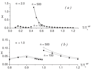
Figure 1: The susceptibility as a function of the temperature $T$ is depicted by (a) $\alpha=2$ and (b) $\alpha=1$, the values of $n$ are indicated in the figure.

The present computational study was carried out on a linear chain with $L=10^{6}$ and $n$ between $10^{2}$ and $10^{3}$, to give effective sizes of the chain of the order from $10^{8}$ to $10^{9}$ particles in according to the Eq.(3), and several values of $\alpha$. Standard techniques are taken into account to compute its normalized autocorrelation function $C(t)$, $C(t)\sim 1\%$, due to the large fluctuations near the critical point.

The magnetic susceptibility as a function of temperature is estimated from the magnetization fluctuation,

$$\chi(T)=\left\{\begin{array}[]{ll}\frac{N}{k_{B}T}(\langle s^{2}\rangle_{n}-\langle|s|\rangle^{2}_{n})&\text{for $T<T_{c}$}\\ &\\ \frac{N}{k_{B}T}\langle s^{2}\rangle_{n}&\text{for $T>T_{c}$},\end{array}\right.$$ (5)

where $T_{c}$ is the critical temperature, $<s>=0$ for $T>T_{c}$. In the Fig.1 typical sets of curves for the magnetic susceptibility are depicted as a function of a reduced temperature $T/T_{c}^{MF}$, where $T_{c}^{MF}=J_{\alpha}^{L}(n)/k_{B}$, where $k_{B}$ is the Boltzmann constant. Range of interactions is given by (a) $\alpha=2$ and (b) $\alpha=1$, and sizes of the central cell are shown for $n=100$ and $500$, for $L=10^{6}$. The total number of particles is given by Eq.(3). The trend of the magnetic susceptibility $\chi(T)$ suggests a discontinuity in Fig.1 and a change of the magnetic ordering phase is related to such property. Circles are obtained from simulations and lines correspond to a linear interpolation of the data in the Fig.1. It is expected that the trend of the magnetic susceptibility becomes a behavior similar to the mean field approximation, this is the magnetic susceptibility has an infinite jump at the critical temperature.

The specific heat is estimated as a function of the temperature from the energy fluctuation, which is given by

$$C(T)=\frac{N}{T^{2}}\left(\langle H^{2}\rangle_{n}-\langle H\rangle^{2}_{n}\right).$$ (6)

In Fig.2, the typical trend of specific heat is depicted. Numerical calculations were carried out for several values of $n$ and $\alpha$; namely, $n=100$, $500$ and $\alpha=1$, $2$. A discontinuity is also observed for the specific heat at critical temperature.

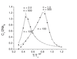
Figure 2: The specific heat as a function of the temperature $T$ is shown. The trend of these functions shows also a discontinuity. The values of $\alpha=1$, $2$ and $n=100$, $500$ are indicated in the figure

The phase transition can be characterized by several ways. A suitable approach to define the critical point in finite system is the Binder method. A typical property is looked for from the profile of the fourth-order cumulant of the magnetizationBinder . A standard behavior of the phase diagram is expected for this kind of system. The Binder cumulant of fourth order is defined as

$$U_{n}=1-\frac{\langle s^{4}\rangle_{n}}{3\langle s^{2}\rangle_{n}^{2}}.$$ (7)

Cumulants $U_{n}$ as a function of the temperature, for several sizes of system $n$, are intersected in a common point. Such point is the critical temperature which depends on values of the parameter $\alpha$. The typical behavior of the Binder cumulant $U_{n}$ (or equivalent quantity $g_{n}=-3U_{n}$ called the renormalized coupling constantprb32 ) is rather stable under critical temperature; however, fluctuations can be important above the critical point. So that, this properties permits to distinguish the critical point by a very simple graphical criteria.

In the Fig.3, the critical temperature is depicted as a function of $1/\alpha$ for the magnetic ordering transition in the thermodynamic limit. Error bars are included to represent a 5 percent or less of the deviation for the obtained values at each point of the critical temperature. Additionally, an inset is included in Fig.3 to show the same fact for $0\leq\alpha\leq 3$. Both pictures are included to emphasize the following features about critical temperature:

• It is close to the mean field one for $\alpha\rightarrow 0$.

• It is lesser than the critical temperature given by the mean field approximation for $\alpha>1$.

• It falls to zero for the short range interaction regime (e.g., nearest neighbor) as it is expected.

• It is depicted as a function of $1/\alpha\rightarrow 0$ to remark that goes to zero while $\alpha\rightarrow\infty$.

• It is depicted the crossover between two known limiting cases.

• It is recovered by the present model the known results for particular values of $\alpha$; namely, $\alpha=1.1$, $1.2$ $1.3$, $1.4$ and $1.5$cssXII and $\alpha=2$SCaIJMPC .

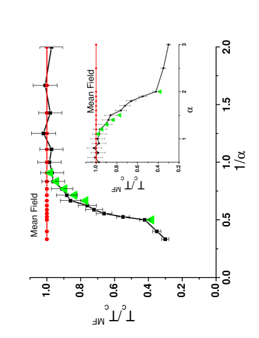
Figure 3: The critical temperature as a function of $1/\alpha$, the inverse of the range of the microscopic interaction, is depicted. The trend of $T_{c}$ goes to zero when $1/\alpha\rightarrow 0$, namely $\alpha\rightarrow\infty$. The inset shows the trend of $T_{c}$ as a function of $\alpha$. Error bars represent a deviation of the 5 percent or less at each point of results.

Table 1: Comparison of our estimation of the critical temperature to previous result in the literatureprb56 .

$\alpha$	$T_{c}$ This work	$T_{c}=(1-\alpha)/2^{\alpha}K_{c}$
1.1	0.9689	0.9797309
1.2	0.9625	0.9438766
1.3	0.9101	0.8951426
1.4	0.8813	0.8367191
1.5	0.86	0.7714285

We can compare the critical temperature with earlier results which are presented in the literature. We have chosen the Ref.prb56 because the authors have made an exhaustive search of the critical couplings $K_{c}$ as a function of $\alpha$ and compare their values to otherstableIII . In order to compare critical temperatures it is necessary to make a simple transformation from Eq.(4) for $N\rightarrow\infty$ given by $T_{c}=(1-\alpha)/2^{\alpha}K_{c}$. The comparison is in the Table 1. In a similar way, for $\alpha=2$, our critical temperature is $0.4221$ and we can compare it to a previous value $0.3816$ obtained from the Ref.cssXII .

In general, according to the Table 1, our estimation for the critical temperature is greater than the value obtained by other author previously. As it is expected that in the limit of short range interactions $T_{c}\rightarrow 0$, it is reasonable to expect that the lower value could be more acceptable. Simulations for larger systems had been carried out in order to obtain accurate results in one dimensionprb56 . However, the numerical work is much more costly due to the enormous number of particles ($n=300000$) in systems, in contrast to the method which has been implemented here, few particles in a cell and a big number of repetitions over all space. If replicas of the central cell are on increase, the time of computation does not practically suffer changes, because such time only depends on the number of particles on the central cell. Sometimes, computation facilities are not sufficient for filling the demands of resources that make simulations of many-body systems; then, it is very important to resort to an alternative numerical way.

On the one hand, a simple theoretical argument given by L. ReichlReichl shows that a finite Ising chain in one dimension with a number of ferromagnetically coupled spins cannot exhibit a phase transition. If the external magnetic field goes to zero the order parameter $\langle s\rangle$ tends also to zero. Hence, no spontaneous nonzero value of the order parameter is possible. On the other hand, another simple theoretical argument given by the same authorReichl shows that the mean field theory predicts a phase transition at a finite temperature for a lattice in one dimension. Both arguments are not opposite between them. In the present point of view, the mean field theory (e.g. $\alpha=0$) approaches to the case of every spin interacts with each other without discriminating over the sites and an Ising chain is the limit whose interactions are very short ranged (e.g. $\alpha=\infty$). In this work, we have discussed the crossover between both limiting cases, with a system of finite ferromagnetically coupled spins that obeys to the Hamiltonian given by Eq.(1).

Summarizing, the inhomogeneity which generally characterizes to systems with interactions with $\alpha\leq 1$ is removed by the scaling $J/J_{\alpha}^{L}(n)$ suggested in Eq.(4), which is used to define the Eq.(1). Thus, if we suppose that the scaling represents the number of nearest neighbor spins, the size of the system (the total number of spins in the chain) is always greater than the such scaling for $0<\alpha\leq 1$. Both values, nearest neighbor and size of the system, are coincident for $\alpha=0$. In this way, we expected that a proper thermodynamic limit can be defined for $\alpha\leq 1$. The scaling is defined and revised by several authors (see for instance Ref.prbCannas and references therein). With such considerations we can repeat the mean field approximation and we hope that the critical temperature comes to be exact. In addition, the most important problem on the thermodynamic behavior related to the systems with long range interactions, it is the strong dependence on the size of systems. It is thought that no standard thermodynamic equilibrium is reached; then, it is crucial to make a suitable choice of the Hamiltonian. However, we have presented a possible way to solve such problem. A nice thermodynamic behavior is obtained from the Hamiltonian suggested in Eq.(1) to Eq.(4). Thermodynamic quantities are not dependent on the size of the system for an appropriated choice of the Hamiltonian.

Finally, in the study and characterization of the phase transition and critical phenomena for systems with arbitrary range interactions, advances and suggestions are always very important to find appropriated models for calculating typical physical quantities.

It is a pleasure to acknowledge partial financial support by grants 1051075 and 1020269 from FONDECYT and Milenio ICM P02-054F. In addition, we would like to thank to D. Barrios for his help in the initial implementation of Monte Carlo procedure.

References

- (1) P. Gambardella, A. Dallmeyer, K. Maiti, M.C. Malagoli, W. Eberhardt, K. Kern, and C. Carbone, Nature 416, 301 (2002).
- (2) J. Dorantes-D vila and G. M. Pastor, Phys. Rev. Lett. 81, 208 (1998).
- (3) J.Shen, R. Skomski, M. Klua, H.Jenniches, S. Sundar Manoharan, and J.Kirschner, Phys. Rev. B 56, 2340 (1997).
- (4) N.D.Mermin and H.Wagner, Phys. Rev. Lett. 17, 1133 (1966).
- (5) S. Cannas, F. Tamarit, Phys. Rev. B 54, 12661 (1996).
- (6) I. F. Herbut, Phys. Rev. B 58 971 (1998).
- (7) P. Gambardella, M. Blanc, H. Brune, K. Kuhnke and K. Kern, Phys. Rev. B 61, 2254 (2000).
- (8) L. van Hove, Physica 16, 137 (1950).
- (9) L. Riechl, “ A Modern Course in Statistical” Mechanics, 2nd. Ed., John Wiley & Sons, INC (1998).
- (10) S. Curilef, Physica A 344, 456 (2004).
- (11) H. Chamati, D. Dantchev, Phys. Rev. E 70, 066106 (2004).
- (12) H. Chamati, N. S. Tonchev, Mod. Phys. Lett. 17, 1187 (2003); J. Phys. A: Math. Gen 33, L187 (2000).
- (13) R. Minieri, Phys. Rev. A 45 3580 (1992).
- (14) E. Luijten and H. W. J. Blöte, Phys. Rev. Lett. 76, 1557 (1996).
- (15) E. Luijten and H. Meingfeld, Phys. Rev. Lett. 86, 5305 (2001).
- (16) E. Luijten and H. W. J. Blöte, Phys. Rev. B 56, 8945 (1997).
- (17) J. O. Vigfusson, Phys. Rev. B 34 3466 (1986).
- (18) P. W. Anderson and J. Yuval, J. Phys. C 4, 607 (1971)
- (19) J. F. Nagle and J. C. Bonner, J. Phys. C 3, 352 (1970)
- (20) E. Luijten, Computer Simulation Studies in Condensed-Matter Physics XII, 86 (2000).
- (21) S. Cannas, C. Lapilli and D. Stariolo, Int. J. Mod. Phys. C 15 115 (2004).
- (22) For a discussion of the behavior of this kind of expressions see for instance Ref. prbCannas and references therein. We remark that, it has been originally proposed as a nonextensive scaling. An alternative model is studied here.
- (23) J.Lekner, Physica A 157, 826 (1989); Physica A 176 485 (1991).
- (24) N.Groenbech-Jensen, Int. J. Mod. Phys. C 6 873 (1996).
- (25) H. Fangohr, A. Price, S. Cox, P. de Groot, G. Daniell, K. Thomas, J. Comp. Phys. 162, 372 (2004).
- (26) S. Curilef, Int. J. Mod. Phys. C 11 629 (2000).
- (27) D. Ruelle, “Statistical Mechanics”, Imperial College Press and World Scientific (1999).
- (28) K. Binder and D. W. Heermann, “Monte Carlo Simulation in Statistical Physics An Introduction”, Fourth Edition Springer (2002).
- (29) M. N Barber, R. B. Pearson, J. L. Richardson, D. Touissant, Phys. Rev. B 32, 1720 (1985).
- (30) The reader can be addressed to the Table III of the Ref.prb56 and to see previous results for .