Equation-free Dynamic Renormalization of a KPZ-type Equation

Abstract

In the context of equation-free computation, we devise and implement a procedure for using short-time direct simulations of a KPZ type equation to calculate the self-similar solution for its ensemble averaged correlation function. The method involves “lifting” from candidate pair-correlation functions to consistent realization ensembles, short bursts of KPZ-type evolution, and appropriate rescaling of the resulting averaged pair correlation functions. Both the self-similar shapes and their similarity exponents are obtained at a computational cost significantly reduced to that required to reach saturation in such systems.

I Introduction

Often we are faced with the study of systems described by a given fine scale, microscopic dynamics, for which we would like to obtain coarse-grained, macroscopic information. Such information can include stationary-states, instabilities, and bifurcations. When continuum equations describing the coarse-grained dynamics are available in closed form, traditional numerical analysis tools can be used to obtain this type of information efficiently. Recently, much work has been devoted to developing tools for addressing such questions in the absence of an explicit coarse-grained description (see PNAS ; GKT ; Manifesto ; ShortManifesto and references therein). These equation-free methods offer the hope of significant savings in storage and run-time costs over direct numerical simulations of the underlying microscopic dynamics. They also allow the study of questions inaccessible to direct simulation, for example the characterization of unstable stationary states. These techniques have been applied to the coarse-grained study of systems described by microscopic evolution rules (kinetic Monte-Carlo, Brownian and molecular dynamics, Lattice-Boltzmann etc., see the references in ShortManifesto ).

These tools can also be applied to problems whose solutions are macroscopically characterized by a symmetry group, such as translational invariance (giving rise to traveling wave solutions). More recently, the techniques have been extended to problems whose macroscopic dynamics exhibits scaling; among these are molecular diffusion chen , models of self-similar transport of random Brownian particles Zou , core collapse in stellar systems Merritt etc. Such problems present challenges, both conceptual and technical, not necessarily found in the simpler traveling-wave problems. For example, since scale-invariance –unlike translational invariance– is never an exact symmetry of the microscopic dynamics, the scaling solutions only exist in an asymptotic limit of large system sizes and long time-scales. Furthermore, one must correctly identify the number of free parameters characterizing the scaling solution.

In this context we consider the scaling behavior of an equation in the KPZ class kpz ; review . This model is a paradigm for a wide class of systems whose correlations exhibit asymptotic scaling. Furthermore, as opposed to the systems studied through equation-free methods to date, the scaling behavior is not present in the first moment of the evolving field, but rather in its correlations; in particular, we will study the scaling solutions for the two-point correlation function. We demonstrate, using the ideas outlined above, how to determine the correlation function self-similar shape and the scaling exponents that characterize it.

The paper is organized as follows: in Section 2 we present the exact form of the equation to be solved, define its correlation function and briefly review its known scaling properties. Following that, in Section 3 we discuss an iterative method for the determination of the self-similar solution and its exponents. Section 4 presents a matrix-free fixed-point approach to the same problem, and we conclude with a discussion in Section 5.

II Preliminaries

The equation we will analyze herein is a discretized form of a modified KPZ equation (in 1+1 dimensions) for the height $h$ of an interface:

$$\dot{h}(x,t)=h^{\prime\prime}(x,t)+\frac{\lambda h^{\prime}(x,t)^{2}}{1+\mu h^{\prime}(x,t)^{2}}+\eta(x,t),$$ (1)

where the noise $\eta$ is $\delta$-correlated in space and time:

$$\langle\eta\rangle = 0$$

$$\langle\eta(x,t)\eta(x^{\prime},t^{\prime})\rangle = S\delta(x-x^{\prime})\delta(t-t^{\prime}).$$ (2)

The $\mu$ term is present to ensure that the equation does not exhibit the finite-time singularity known to arise for sufficiently large $\lambda$ in the unmodified $\mu=0$ equation yuhai . Dimensional analysis shows that $\mu$ does not change the scaling behavior of the system.

In discretized form, our equation reads

$$h^{t+\Delta t}_{i}=h_{i}^{t}+\Delta t\left[h^{t}_{i+1}-2h^{t}_{i}+h^{t}_{i-1}+\frac{\lambda(h^{t}_{i+1}-h^{t}_{i-1})^{2}}{4+\mu(h^{t}_{i+1}-h^{t}_{i-1})^{2}}+\eta^{t}_{i}\right]$$ (3)

with $\langle\eta^{t}_{i}\rangle=0$, $\langle\eta^{t}_{i}\eta^{t^{\prime}}_{j}\rangle=S\delta_{t,t^{\prime}}\delta_{i,j}/\Delta t$. We work in a periodic box of length $L$. In the following, we take $\mu=1$, $S=1/12$, $\Delta t=0.05$. It is customary to start simulations ($t=0$) from a flat interface $h^{0}_{i}=0$. It is convenient to define the average height $\bar{h}^{t}\equiv\frac{1}{L}\sum_{i=0}^{L-1}h^{t}_{i}$ and the reduced height $\hat{h}^{t}_{i}\equiv h^{t}_{i}-\bar{h}^{t}$. Since a flat interface is stable, $\langle\hat{h_{i}}\rangle=0$, and the basic object of interest is the two-point correlation function:

$$G^{t}(d)=\frac{1}{L}\sum_{i=0}^{L-1}\langle\hat{h}^{t}_{i}\hat{h}^{t}_{i+d}\rangle$$ (4)

or, equivalently, its (discrete) Fourier transform:

$$G^{t}_{K}=\frac{2}{L}\sum_{d=0}^{L/2}e^{2\pi iKd/L}G^{t}(d)$$ (5)

where $K=kL/(2\pi)=1,\ldots,L/2$ and $k$ is the momentum.

Let us briefly review the basic known scaling properties of $G^{t}_{K}$ review . For intermediately large wavenumber $K$, $K^{*}(t)\ll K\ll L/2$, $G^{t}_{K}$ falls like a power-law for increasing $K$, $G^{t}_{K}\sim C/K^{2\alpha+1}$, where $C$ is independent of $t$. At small $K\ll K^{*}(t)$, the power-law growth is cut off, and $G$ approaches a finite limiting value as $K\to 0$ with zero derivative. The crossover length scale, $1/K^{*}(t)$, grows with time as $t^{1/z}$, until the saturation time when $1/K^{*}(t)\sim L$. This saturation time thus grows with the system size as $L^{z}$. At small $K\ll K^{*}(t)$, $G$ saturates at a value which grows in time like $t^{(2\alpha+1)/z}$, again until the saturation time. The values of the exponents $\alpha$ and $z$ in this one-dimensional system are known analytically , $\alpha=1/2$, $z=3/2$. Putting this all together, $G$ has the scaling form

$$G^{t}_{K}=t^{(2\alpha+1)/z}f(Kt^{1/z}).$$ (6)

where the function $f(x)$ approaches a constant for small arguments and decays as $1/x^{2\alpha+1}$ for large $x$.

III Solution by Direct Iteration.

Our goal is to find a self-consistent $G_{K}^{t}$ with the correct scaling properties, i.e. find the function $f(.)$ in Eq. 6 above. Roughly speaking, if we knew the exact $G_{K}^{t}$, we could use this knowledge to generate an ensemble of initial $h$ fields at some time $t_{0}$, conditioned on this $G$. We could then evolve each of these initial $h$’s forward in time to some $t_{f}$, and calculate $G$ at this later time. The new $G$ should then simply be a rescaled version of the original $G$. This scaling condition is what we use to determine $G$.

There are a number of caveats that need to be expounded at this point. Some of these are technical in nature, involving the details of the algorithm used to actually find $G$. Two, however, involve matters of principle. The first caveat is that the full statistical solution is not uniquely determined solely by the two-point function $G$. In principle, a complete solution implies knowledge of all higher-order correlations as well. However, we posit that the dynamics is such that the higher-order correlators relax much more quickly than the two-point function itself. If this is true, there will be a short transient during which time the system will reconstruct all the higher-order correlations (will “heal”) while $G$ itself does not change much. In effect, this is an assumption of separation of time scales between different order correlators. Thus, to determine the solution, we compare not $G$ at times $t_{0}$ and $t_{f}$, but at times $t_{I}$ and $t_{f}$, where $t_{I}$ is an intermediate time chosen so that the higher-order correlators have had time to become slaved to $G$ (recover their correct values conditioned on the given $G$).

The second caveat is that $G$ exhibits the desired scaling properties only asymptotically. At the smallest scales, the underlying lattice ruins scale-invariance. More serious, however, is the fact that for short times and small scales, the scaling properties of $G$ are those of the Edwards-Wilkinson, i.e., the $\lambda=0$ model EW . Only for sufficiently large times is the interface sufficiently rough for the nonlinearity to determine the scaling. Starting simulations from a flat interface and evolving for time $t_{0}$ brings the interface to some scale of roughness parametrized by $t_{0}$. Our procedure will converge on the particular member of the scaling family that has this characteristic roughness scale; needless to say, all members of the scaling family (at large enough scales !) can be directly reconstructed. As we will see in more detail below, unless the initial time $t_{0}$ (alternatively, the initial roughness scale) is large enough, our results will be contaminated by the short-time, small scale Edwards-Wilkinson behavior. Only if our working scale is large enough for the asymptotically self-similar behavior to have set in, does our process make sense. In practice this means that we must test the working roughness scale (alternatively, the working $t_{0}$) to confirm that both the self-similar shape and the exponents have converged. As we increase $t_{0}$, we will of course have to increase $L$ accordingly, so that we continue to capture the full self-similar structure of $G$.

We now move on to the technical details of the calculation. The primary issue to address is how to solve the fixed-point equation embodying the scale invariance condition. We will do this in two different ways. The first is by successive substitution. Here we just perform repeated cycles of forward integration, followed by rescaling to the original time (roughness). The second is via a fixed point Newton-type procedure, which we describe in the next section.

Direct iteration proceeds as follows. We start by integrating the system forward from a flat interface at $t=0$ to some $t_{0}$. We then calculate $G^{0}_{K}$. It is straightforward to generate configurations $h_{i}$ conditioned on this $G^{0}_{K}$ (to “lift” from $G$ to $h$). All we have to do is to remember that $G_{K}$ is the expected value of $|h_{K}|^{2}$. Thus, we generate a Gaussian random number with zero mean and variance $G^{0}_{K}$, and multiply by a random phase to obtain an $h_{K}$. An inverse Fourier transform gives us our desired $h_{i}$. We generate some number, (typically 32,000) of such initial configurations and integrate each forward in time to $t_{f}$, which we take to be $t_{f}=2t_{0}$, and measure $G^{f}_{K}$. We also measure $G^{I}_{K}$ at an intermediate time $t_{I}=3t_{0}/2$. From these measurements we construct the functions $G^{0}(K),G^{I}(k)$ and $G^{f}(k)$ (see below for details). We now need to rescale $G^{f}(k)$ back to the original roughness scale (or time $t_{0}$). We do this is two steps. We first determine, for each measuring time, a typical small $k$ scale, $k_{1/2}$ by the condition $G({k_{1/2}})=G(0)/2$. We next rescale wavenumbers at times $t_{I}$ and $t_{f}$ by the factors $f_{k}^{I,f}=k_{1/2}^{0}/k_{1/2}^{I,f}$, respectively; this “aligns” their rescaled large scale behavior. We next rescale $G^{I}$ and $G^{f}$ by factors $f_{G}^{I,f}=G^{I,f}({k_{B}/f_{k}^{I,f}})/G^{0}({k_{B}})$ (where $k_{B}=\sqrt{L/2}$ is the geometric mean of the smallest and largest wavenumbers) so that their large wavenumber behavior coincides with that of $G^{0}$. For the self-similar shape, the function $G^{f}(k/f_{k}^{f})/f_{G}^{f}$ should reproduce our original function $G^{0}(K)$. In practice, it gives us a new starting point for another round of iteration; in our problem the self-similar solution is stable, and this procedure rapidly converges, so that in fact the differences are only due to fluctuations. If the problem was truly (as opposed to asymptotically) self-similar, upon convergence to the self-similar solutions, the scaling factors $f_{K}^{I,f}$ and $f_{G}^{I,f}$ could be used to estimate the effective scaling exponents $\alpha$ and $z$:

$$z = \ln(t_{f}/t_{I})/\ln(K_{1/2}^{I}/K_{1/2}^{f})=\ln(t_{f}/t_{I})/\ln(f_{K}^{f}/f_{K}^{I})$$

$$\alpha = \frac{1}{2}\left(\frac{\ln(f_{G}^{f}/f_{G}^{I})}{\ln(f_{K}^{f}/f_{K}^{I})}-1\right)$$ (7)

Because the self-similarity is only asymptotic, three successive times are in fact needed to estimate the exponents. This procedure constitutes the equation-free implementation of dynamic renormalization (see e.g. the classical references McLaughlin ; LemesurierA ; LemesurierB , as well as our template-based approach discussed in Aronson ; Rowley2 ).

The last point we need to cover is how we convert our measured $G_{K}$ into a function $G(k)$. We use a relatively low-dimensional description of the function G(k); in particular, we fit a cubic spline to $log(G_{K})$ throughout the whole range, with knots approximately equally spaced in $log(K)$; this provides an adequate description with $O(10)$ degrees of freedom.

An example of the results of this procedure are shown in Fig. 1, where one cycle of the iteration is shown. We see that indeed $G(k)$ is recovered to quite good accuracy by our integration and rescaling, except for the very largest $k$’s, where the zero-slope condition imposed by the discreteness of the lattice is evident in the original $G$, but not in its rescaled version.

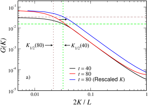
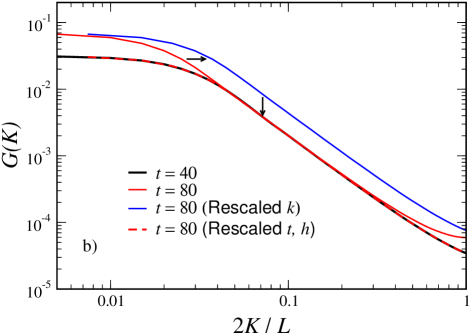
Figure 1: The iteration cycle for $\lambda=5$, $L=400$, $t_{0}=40$. a) $G(K,t)$ for $t=40$ and $t=80$, with their respective $K_{1/2}$’s noted, together with $G(K,80)$ after rescaling of $K$ to align its $K_{1/2}$ with $G(K,40)$. b)$G(K,40)$ and $G(K,80)$, together with $G(K,80)$ after rescaling of $K$ and after rescaling of both $k$ and $h$ to collapse it onto $G(K,40)$.

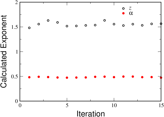
Figure 2: Calculated values of the exponents $z$, $\alpha$ vs. iteration for $\lambda=5$, $L=400$, $t_{0}=40$.

We present in Fig. 2 a graph of the estimated exponents as a function of iteration number, for some particular value of $t_{0}$ and $L$. We see that the iteration is quite stable, albeit with sizable statistical fluctuations. In Fig. 3(a-b), we present the cumulative average over iterations of the estimated exponents, as a function of iteration number, for various sets of $t_{0}$ and $L$. What is remarkable is that the calculation essentially converges immediately, to the precision we can measure. Our procedure allows us work at an intermediate scale where we can see simultaneously the rapid saturation of the correlation function at short length scales and the growth at the coarse scales, tracking the shift of the crossover between these two regimes while this evolution is still relatively fast; approaching the ultimate shape while the interface evolves to coarser scales would take a significantly longer computational time (the coarser the scale, the longer the time). It is this “shape evolution at constant scale” that underpins the computational savings of the method. We see that increasing $t_{0}$ (alternatively, the working roughness scale) brings the measured value of $z$ down much closer to its asymptotic value of $3/2$. Since the value of $z$ for the Edwards-Wilkinson model is $2$, we interpret this as indicating the contamination of our measurement by the crossover from Edwards-Wilkinson behavior at short scales. In Fig. 4, we present for comparison the data for the Edwards-Wilkinson model. Here we immediately obtain values very close to the expected $z=2$, $\alpha=1/2$, as the only violation to scaling comes from the very short scale lattice effects.

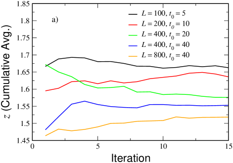
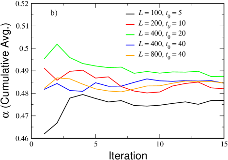
Figure 3: Cumulative average of the estimated exponents (a) $z$; and (b)$\alpha$ as a function of iteration number for $\lambda=5$ and various pairs of $t_{0}$, $L$.

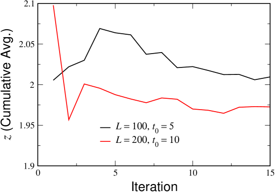
Figure 4: Cumulative average of the estimated exponent $z$ as a function of iteration number for the Edwards-Wilkinson model ($\lambda=0$) and two sets of $t_{0}$, $L$.

IV Newton-GMRES Fixed Point Solution

A direct iteration procedure is, of course, not guaranteed to converge; the self-similar solution may not be stable for the system and parameter values of interest. Even if it is stable, one needs to start in its basin of attraction, and the rate of approach will asymptotically depend on the local linearization characteristics of our fixed point formulation. It is therefore desirable to develop approaches that do not rely on the stability of the fixed point, and the Newton method is the obvious choice. Lack of an explicit macroscopic equation means that the Jacobian involved in Newton iterations is not explicitly available. In principle one could estimate the Jacobian using finite differences; yet, especially for large scale and noisy problems, such an estimation will be both prone to error and very costly. Krylov-subspace methods, such as GMRES, have been devised for the iterative solution of linear equations; they are based on the evaluation of matrix-vector products of the system Jacobian with a sequence of algorithmically determined vectors. When the Jacobian is not explicitly available, matrix vector products can be estimated in a matrix-free fashion from nearby function evaluations - this is the basis for matrix-free Newton-Krylov-GMRES algorithms Kelley . Such algorithms are naturally suited to the fixed point problems arising in our equation-free renormalization scheme - lifting from nearby two-point correlation functions, evolving through the KPZ dynamics, and rescaling the resulting averaged two-point correlations results in an estimate of the action of the Jacobian of our fixed point problem. This type of iteration is often particularly well suited for problems with a separation of time scales Liang .

We used Newton-Krylov GMRES iteration to find the shape of the fixed point of the KPZ renormalization problem; the operating parameters were $L=400,\lambda=5$, and a short burst of time simulation, $\Delta t=5$, was used to calculate the evolved shape. Cubic spline interpolation was again used in the construction of the function $G(k)$. All the data were averaged over $96000$ replica initializations consistent with this $G(k)$. The initial guess was obtained by starting from a flat interface and evolving for time of $t_{0}=5$. As shown in Fig. 4, it took roughly three iterations for the plotted norm of the residual to decrease by one order of magnititude. The resulting fixed point is visually indistinguishable from the one arrived at by direct substitution, and the same scaling exponents, within the fluctuation bounds, are recovered. The Newton-based process is not computationally efficient in problems such as this, where the self-similar solution is strongly attracting; it would become advantageous, however, in cases where the self-similar solution is very slowly attracting, or simply unstable, when direct iteration will not converge at all.

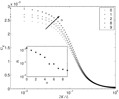
Figure 5: GMRES iterations to find the fixed shape ($L=400,\lambda=5,\Delta=5,N=96000$) The inset shows the residual $R$ as a function of iteration number.

V Discussion and Conclusions

We presented a computational approach to finding self-similar solutions for the statistics of a KPZ-type stochastic evolution equation. This was accomplished without an explicit, closed form of an equation governing the dynamics of these statistics (in particular, the two-point correlation function); we estimated this unavailable equation on demand using short bursts of appropriately initialized direct simulations. The approach was successful in reproducing the known scaling behavior of the model. One of the important features of the computation was the detection of the signature of Edwards-Wilkinson scaling in the data when the working scales were not chosen large enough (due to asymptotic self-similarity). In our current implementation we used two local conditions (“templates”, Rowley1 ; Rowley2 ) to implement the two rescalings, those of the stretching of the wavenumber (or reshrinking of the length scale) and the scaling down of $G_{K}$ (equivalently the field variable amplitude $h_{K}$). It would be preferable to employ non-local conditions, making the computation more robust to local fluctuations through averaging.

Perhaps the most important assumption of the equation-free approach is that an equation exists and closes at a chosen level of description; here we assumed that the appropriate level was the two-point correlation function, and that higher order correlations either do not affect this evolution or become quickly slaved to it. It is known edwards-schwartz that in one spatial dimension the exponents are insensitive to variations in the third and higher order correlators; this appears not to be true in higher dimensions. In our computational experiments we found that third order correlations did not become quickly slaved to two-point correlations (over times comparable to the evolution of the two-point correlation itself); since we worked in 1+1 dimension, this is consistent with the above observation. In higher dimensions, it is not clear that an equation does indeed close in terms of only the two-point correlation function; testing this hypothesis would be an important first task to pursue with our approach. Computational approaches to initializing “fast” variables consistently with slow ones (alternatively, on a manifold parametrized by the slow ones) have long been known in computational chemistry (Ciccotti ; Valleau ), and their use in an equation-free context is discussed, for example, in GearK .

In this paper we used a KPZ-type SDE as our “inner”, fine scale solver. The procedure is identical if the SDE solver is substituted by, for example, a kinetic deposition model; the computation of coarse self-similar solutions for such models is underway. For some of these, such as ballistic aggregation, we do not anticipate any difficulties; for other, more highly constrained models, e.g. the restricted SOS model review the lifting operation should be nontrivial. In the case of stable self-similar solutions additional equation-free techniques, such as coarse projective integration GK1 ; GK2 can be used to accelerate the computation of self-similar dynamics.

An important test of the approach will be its ability to compute and characterize the unstable fixed point that is known to exist in $d\geq 3$ dimensions; this is a case where the Newton-GMRES procedure would be crucial.

Acknowledgements This work was partially supported by NSF and DOE (USA) and by the Israel Science Foundation.

References

- (1) K. Theodoropoulos, Y.-H. Qian and I.G. Kevrekidis, Proc. Natl. Acad. Sci. 97, 9840 (2000).
- (2) C. W. Gear, I.G. Kevrekidis and C. Theodoropoulos, Comp. Chem. Engng. 26, 941 (2002).
- (3) C. W. Gear, J. M. Hyman, P. G. Kevrekidis, O. Runborg and K. Theodoropoulos, Comm. Math. Sciences, 1, 715 (2003); original version can be obtained as physics/0209043 at arXiv.org.
- (4) I. G. Kevrekidis, C. William Gear and G. Hummer, A.I.Ch.E Journal, 50, 1346 (2004).
- (5) L. Chen, P. G. Debenedetti, C. W. Gear and I. G. Kevrekidis, J. Non-Newtonian Fluid Mech. 120, 215 (2004).
- (6) Y. Zou, I. G. Kevrekidis and R. Ghanem, Phys. Rev. E, submitted; math.DS/0505358 in arXiv.org.
- (7) A. Szell, D. Merritt and I. G. Kevrekidis, Phys. Rev. Lett., submitted; can be found as astro-ph/0504546.
- (8) M. Kardar, G. Parisi and Y.-C. Zhang, Phys. Rev. Lett. 56, 889 (1986).
- (9) For a general review of the KPZ equation and related systems, see T. Halpin-Healy and Y.-C. Zhang, Physics Reports 254, 215 (1995).
- (10) Y. Tu, private communication.
- (11) S. F. Edwards and D. R. Wilkinson, Proc. Roy. Soc. London A381, 17 (1982).
- (12) D.W. McLaughlin, G.C. Papanicolaou, C. Sulem and P.L. Sulem, Phys. Rev. A, 34, 1200 (1986).
- (13) B.J. LeMesurier, G.C. Papanicolaou, C. Sulem and P.L. Sulem, Physica D, 31, 78 (1988).
- (14) B.J. LeMesurier, G.C. Papanicolaou, C. Sulem and P.L. Sulem, Physica D, 32, 210 (1988).
- (15) D.G. Aronson, S.I. Betelu, I.G. Kevrekidis, see arxiv.org nlin/0111055, (2001).
- (16) C.W. Rowley, I.G. Kevrekidis, J.E. Marsden and K. Lust, Nonlinearity, 16, 1257 (2003).
- (17) C.T. Kelley, Iterative Methods for Linear and Nonlinear Equations, (SIAM, 1995).
- (18) C. T. Kelley, I.G. Kevrekidis, Q. Liang, submitted to SIADS (2004); math.DS/0404374 at arXiv.org.
- (19) C.W. Rowley and J.E. Marsden, Physica D, 142, 1 (2000).
- (20) M. Schwartz and S. F. Edwards, Europhys. Lett. 20, 301 (1992).
- (21) J.P. Ryckaert, G. Ciccotti, and H. Berendsen, J. Comp. Phys., 23, 327 (1977).
- (22) G. M. Torrie, J. P. Valleau, Chem. Phys. Letters, 28, 578 (1974).
- (23) C. W. Gear, T. J. Kaper, I. G. Kevrekidis and A. Zagaris, SIADS, can be found as Physics/0405074 at arXiv.org.
- (24) C. W. Gear and I. G. Kevrekidis, , SIAM J. Sci. Comp. 24(4) 1091 (2003).
- (25) C. W. Gear and I. G. Kevrekidis, J. Comp. Phys. 187(1) 95-109 (2003).