A Simple Computer Model for Liquid Lipid Bilayers

Abstract

We present a simple coarse-grained bead-and-spring model for lipid bilayers. The system has been developed to reproduce the main (gel–liquid) transition of biological membranes on intermediate length scales of a couple of nanometres and is very efficient from a computational point of view. For the solvent environment, two different models are proposed. The first model forces the lipids to form bilayers by confining their heads in two parallel planes. In the second model, the bilayer is stabilised by a surrounding gas of “phantom” solvent beads, which do not interact with each other. This model takes only slightly more computing time than the first one, while retaining the full membrane flexibility. We calculate the liquid–gel phase boundaries for both models and find that they are very similar.

,

1 Introduction

A biological membrane (e.g. the cell wall or walls between different compartments in the cell) consists mainly of a bilayer of amphiphilic lipids. It forms an impermeable barrier between watery environments that may have different chemical characteristics and it is extremely flexible. This is generally believed to be due to the liquid state of the bilayer. In this state, the hydrophobic tails of the lipids are disordered and the whole bilayer shows a very low viscosity in the membrane plane [1].

However, for many lipids the main transition – where the bilayer undergoes a phase transition to the gel phase with a much higher viscosity and ordered tails – is close to body temperature (e.g. $\approx 41^{o}C$ in a pure DPPC bilayer). It seems reasonable to assume that this proximity of the transition carries some biological importance, e.g. for lipid-mediated protein-protein interactions or for the formation of rafts and domains on the nanometre scale. Therefore it is interesting to study the properties of the transition.

The liquid–gel transition of the bilayer is mainly characterised by a change of the in-plane viscosity, the area of the bilayer per lipid and the lipid tail ordering. These effects take place on an intermediate length scale of a few up to a few tens of nanometres and involve some ten thousands of atoms. Only recently it has become possible to access these length scales by experimental techniques ([2, 3]).

Computer simulations have proved to be excellent tools for understanding the nature of phase transitions in this type of systems. However, on current computer hardware, systems of a size of some ten thousands of atoms can not be studied in detail by simulations on the atomic level. To bridge the gap between the length scales, we propose a simple, robust, coarse-grained model of a lipid bilayer. It is devised to reproduce the liquid–gel transition while spending very little computing time the solvent environment. The model does not attempt to catch the chemical details of any specific lipid, but instead describes the generic characteristics of a bilayer that undergoes the main transition.

Comparable models have been used before by Götz and Lipowsky [4], Sintes and Baumgärtner [5, 6, 7], Noguchi and Takasu [8, 9, 10, 11, 12] and Farago [13]. Of these models, only the latter has been shown to exhibit the liquid–gel phase transition. Otherwise, the models differ mainly in the treatment of the solvent environment. A good model of the solvent environment is required to keep the bilayer stable in the liquid phase. Götz and Lipowsky employ a rather costly model of explicit solvent beads, whereas Sintes and Baumgärtner use a surface potential similar to the surface potential solvent model proposed in this article. The models of Noguchi and Takasu and of Farago both are solvent-free, i.e. they do not use an explicit solvent model, which makes them very efficient. Instead, they use elaborate lipid–lipid potentials to acquire liquid bilayer stability. The phantom bead solvent model described in this article is as efficient as these solvent-free models. However, it is simpler and presumably more robust. The phantom beads have a simple physical interpretation.

The model has been tested using a constant-pressure Monte-Carlo (MC) simulation, but it should also be possible to use it in Molecular Dynamics (MD) computer simulations.

2 Model

The bilayer model consists of two subparts – the model of the lipids that form the bilayer (Section 2.1), and the solvent environment model (Section 2.2). The solvent environment is required to keep the liquid bilayer together. The model is robust towards different solvent models in the sense that the exact form of the model solvent seems to be relatively unimportant. In the following, we will present two very different solvent environment models, both of which enable the bilayer to undergo the liquid–gel transition and maintain a stable liquid phase, while still being efficient when it comes to computing.

2.1 Lipid Model

The lipid model used in this work was derived from a successful coarse-grained model for Langmuir monolayers that was able to reproduce the generic phase diagram of such monolayers in great detail [14, 15].

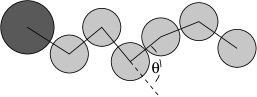
Figure 1: Sketch of a lipid.

A lipid in the model system consists of six tail beads and one slightly larger head bead (see Figure 1). All lipid beads interact via a truncated 12-6-Lennard-Jones potential of the form :

$$V_{\mathrm{LJ}}^{\mathrm{shifted}}(r)=\left\{\begin{array}[]{ll}0&\mathrm{,if~{}}r>r_{\mathrm{cutoff}}\\ V_{\mathrm{LJ}}(r)-V_{\mathrm{LJ}}(r_{\mathrm{cutoff}})&\mathrm{,otherwise}\\ \end{array}\right.$$ (1)

with

$$V_{\mathrm{LJ}}(r)=\epsilon\left({\left(\frac{\sigma}{r}\right)}^{12}-2{\left(\frac{\sigma}{r}\right)}^{6}\right)$$ (2)

For tail-tail interactions, the cutoff is $r_{\mathrm{cutoff}}=2\sigma$, the potential thus has an attractive contribution. Head beads interact with each other and with tail beads via a soft-core potential, i.e. the purely repulsive core of the 12-6-Lennard-Jones potential $V_{\mathrm{LJ}}^{\mathrm{shifted}}$ with a cutoff radius of $\sigma$.

The adjacent beads of a lipid chain are bound to each other by a FENE (finite extensible nonlinear elastic, see Equation 3) type spring potential that limits the maximal and minimal bond length. Additionally, a bond-angle potential (Equation 4) favours stretched chain conformations.

$$V_{\mathrm{FENE}}(r)=-\frac{1}{2}\epsilon(\Delta r_{\mathrm{max}})^{2}\>\log\left(1-\frac{r-r_{0}}{\Delta r_{\mathrm{max}}}^{2}\right)$$ (3)

$$V_{\mathrm{BA}}(\theta)=\epsilon\>(1-\cos\theta)$$ (4)

The length of the chains (i.e. the number of tail beads) and the interaction parameter of the bond-angle potential $V_{\mathrm{BA}}$ are adapted to model lipids with a fully saturated acyl chain of 16 to 18 carboxyl groups [16, 14, 15]. The interaction potentials and parameters of the lipid model are summarised in table 1. All lengths in the system are measured in units of the tail–tail-potential Lennard-Jones parameter $\sigma$, the energy unit is $k_{B}T$.

	Potential	Parameters
tail–tail	$V_{\mathrm{LJ}}^{\mathrm{shifted}}(|\vec{r}|)$	$\epsilon=1$, $\sigma=1$, $\frac{r_{\mathrm{cutoff}}}{\sigma}=2$
head–tail	$V_{\mathrm{LJ}}^{\mathrm{shifted}}(|\vec{r}|)$	$\epsilon=1$, $\sigma=1.05$, $\frac{r_{\mathrm{cutoff}}}{\sigma}=1$
head–head	$V_{\mathrm{LJ}}^{\mathrm{shifted}}(|\vec{r}|)$	$\epsilon=1$, $\sigma=1.1$, $\frac{r_{\mathrm{cutoff}}}{\sigma}=1$
bond-length	$V_{\mathrm{FENE}}(|\vec{r}|)$	$\epsilon=100$, $r_{0}=0.7$, $\Delta r_{\mathrm{max}}=0.2$
bond-angle	$V_{\mathrm{BA}}(\theta)$	$\epsilon=4.7$

Table 1: Summary of the interaction potentials of the lipid model. $\vec{r}$ is the centre-to-centre distance vector of two beads, $\theta$ is the bond angle of three adjacent beads (as depicted in figure 1). Parameters are taken from [15].

2.2 Solvent Environment Models

In the first solvent environment model used in this work, the bilayer is defined by two parallel planes. The lower plane is the $x$-$y$-plane itself, the upper plane is shifted by $z_{\mathrm{upper}}>0$. The tail beads of the bilayer are confined between the planes by the surface potential $V_{\mathrm{ST}}$ (Equation 5), while the head beads are forced to stay above the upper plane resp. below the lower plane by $V_{\mathrm{SH}}$ (see Equation 6, with the parameters $\epsilon=10$, $r_{0}=0$ and $\Delta r_{\mathrm{max}}=0.5$ for $V_{\mathrm{FENE}}$).

$$V_{\mathrm{ST}}(r)=\left\{\begin{array}[]{ll}V_{\mathrm{FENE}}(z)&\mathrm{,if~{}}z<0\\ V_{\mathrm{FENE}}(z-z_{\mathrm{upper}})&\mathrm{,if~{}}z>z_{\mathrm{upper}}\\ 0&\mathrm{,otherwise}\\ \end{array}\right.$$ (5)

$$V_{\mathrm{SH}}(z)=\left\{\begin{array}[]{ll}V_{\mathrm{FENE}}(z)&\mathrm{,if~{}}0<z<\frac{1}{2}z_{\mathrm{upper}}\\ V_{\mathrm{FENE}}(z-z_{\mathrm{upper}})&\mathrm{,if~{}}\frac{1}{2}z_{\mathrm{upper}}<z<z_{\mathrm{upper}}\\ 0&\mathrm{,otherwise}\\ \end{array}\right.$$ (6)

Unfortunately, the bilayer is not flexible, so the model is useless for the simulation of phenomena that involve any membrane deformations, such as undulations, hydrophobic mismatch effects of membrane integral proteins etc.

On the other hand, this solvent environment model is very easy to implement and is also very efficient when it comes to computing, as it will add only a single term per bead to the energy sum.

Therefore, another solvent environment model was developed, which retains the full membrane flexibility, while adding only a small computational overhead. In this “phantom solvent bead model”, the solvent is represented by explicit solvent beads. These beads behave exactly like additional, unbound head beads (i.e.it has a purely repulsive soft-core interaction with the lipid beads), except that they do not interact with each other.

This has a number of advantages. First, the model is still computationally efficient, as only those solvent beads that are actually close to the bilayer significantly contribute to the computing time. Furthermore, the model has no solvent artefacts, as the solvent can not develop any internal structure. Therefore, the model can employ periodic boundary conditions perpendicular to the bilayer and only a relatively thin layer of solvent beads is needed to ensure that the bilayer does not interact with itself via the periodic boundary conditions. If one uses a thicker layer of phantom solvent beads, the pressure of the system can be easily measured, as the ideal gas equation of state holds for the phantom solvent beads far from the bilayer.

3 Simulation Details

The system was simulated using a constant pressure Monte-Carlo (MC) simulation with periodic boundary conditions in all directions. We used standard single bead moves as well as collective volume moves that stretched or squeezed the whole system in $x$-, $y$- or $z$-direction independently, the effective Hamiltonian being

$$H_{\mathrm{eff}}=\Phi(r)+pV-Nk_{B}T\log(V)$$ (7)

where $\Phi(r)$ is the potential energy of all beads, $p$ is the desired pressure, $V$ is the (fluctuating) volume, $T$ is the temperature of the system and $N$ is the number of beads in the system. $H_{\mathrm{eff}}$ results from a Laplace transformation of the $NVT$-Hamiltonian.

We note, that in the case of the surface potential solvent model, the volume of the system $V$ is, strictly speaking, not well-defined. However, this does not cause problems, because $V$ in the effective Hamiltonian just sets the length scales of the system in the different directions. Therefore, we can rewrite the effective Hamiltonian for the surface potential model as

$$H_{\mathrm{eff}}^{\mathrm{surface}}=\Phi(r)+pL_{x}L_{y}z_{\mathrm{upper}}-Nk_{B}T\log(L_{x}L_{y}z_{\mathrm{upper}})$$ (8)

where $L_{x}$ and $L_{y}$ are the system sizes in $x$ and $y$-direction respectively [17, pages 103ff].

The simulation runs performed for this work involved 288 lipids, which were initially set up perpendicular to the $x$-$y$-plane with 144 lipids in each layer, the heads forming a two-dimensional triangular grid. In the case of the phantom solvent bead model, up to 16 666 solvent beads were distributed randomly outside the bilayer.

The total run length varied between 500 000 and 2 000 000 Monte-Carlo steps (MCS), where one MCS includes one volume move in each direction and $N$ single bead moves. The maximal move ranges for the different moves were adapted to yield an acceptance rate of approximately 30 % in a simulation pre-run of 10 000 to 50 000 MCS.

4 Results

4.1 Liquid–gel phase transition

Figures 2 and 3 show typical snapshots of systems with both solvent environment models in the gel and liquid phases. The gel phase is characterised by a strong ordering the lipid tails, a high bilayer thickness and a small area per lipid of the bilayer, while the liquid phase exhibits disordered tails, a much lower bilayer thickness and a larger area per lipid head.

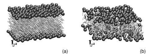
Figure 2: Snapshots of the bilayer model with surface potential in the gel ((a), $p=1.0$, $T=0.9$) and liquid ((b), $p=1.0$, $T=1.0$) phase. The tail beads have been replaced by tubes for better visualisation.

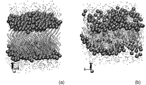
Figure 3: Snapshots of the bilayer model with phantom solvent beads in the gel ((a), $p=1.0$, $T=0.9$) and liquid ((b), $p=1.0$, $T=1.0$) phase. The tail beads have been replaced by tubes and the phantom solvent beads by small spheres for better visualisation.

The lipid tail ordering can be expressed by the nematic order parameter $S$ of the lipid chains which is given by the largest eigenvalue of the matrix

$$S_{ij}=\frac{1}{2N}\sum_{n=1}^{N_{\mathrm{lipids}}}(3x_{i}^{(n)}x_{j}^{(n)}-\delta_{ij})$$ (9)

where $x_{i}$ and $x_{j}$ are the components of the end-to-end vectors of the $N_{\mathrm{lipids}}$ lipid chains in a configuration [18]. As shown in Figure 4, it drops considerably at the phase transition. Figure 5 displays the jump of the measured area per lipid $A$ at the phase transition.

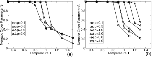
Figure 4: Plot of the nematic order parameter $S$ of the system with surface potential (a) and phantom solvent beads (b).

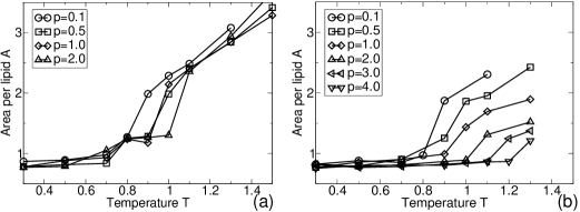
Figure 5: Plot of the area per lipid A of the system with surface potential (a) and phantom solvent beads (b).

4.2 Phase Diagrams

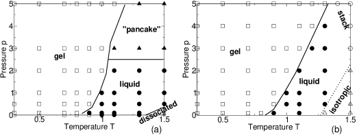
Figure 6: Phase diagrams of the bilayer model with surface potential (a) and with phantom solvent beads (b). The symbols indicate parameter values for which simulations have been carried out. Open squares: gel phase, closed circles: liquid phase, closed triangles: “pancake” phase, stars: dissociated monolayers, open circles: spontaneous formation of bilayer stacks, open triangles: disordered isotropic phase. The lines are eye-guides only and indicated the approximate location of the phase boundaries.

Figure 6 depicts the phase diagrams of the bilayer model obtained from the simulations with both solvent environment models. The liquid–gel transition can be observed clearly in both systems at low to intermediate pressures.

At higher temperature and lower pressure, the bilayer breaks up into two dissociated monolayers. At higher pressures, the surface potential model develops an unphysical “pancake” phase. In this phase, the distance of the two layers ($z_{\mathrm{upper}}$) almost becomes zero and the lipids spread over a large area, as in a two-dimensional gas.

In the phantom solvent bead model, the liquid–gel phase transition can be observed over a wider pressure range. At lower pressure and higher temperature, the liquid bilayer dissolves and forms an isotropic phase. At higher pressure and higher temperature, we have also observed the spontaneous formation of a stack of two liquid bilayers.

5 Conclusions and Discussion

From the Langmuir monolayer model used in our group before [15, 19, 14] we learned, that the key to the successful reproduction of the generic phase behaviour of lipid systems is the qualitatively correct modelling of the translational and conformational degrees of freedom of the lipids. Furthermore, the attractive part of the tail-tail potential is crucial for the liquid phase and the liquid–gel transition. As long as this is taken into account, however, the liquid–gel transition is robust towards changes in the exact form and parameters of the interaction potentials between the lipids. It is to be expected that these results also hold for the bilayer model.

As far as the solvent environment model is concerned, we can deduce that the existence and location of the transition is almost not influenced by the solvent model. In contrast to this, the stability of the liquid phase does depend on the solvent. However, it seems to be sufficient to introduce “phantom beads” that basically probe the free solvent-accessible volume to create a stable, liquid bilayer.

Furthermore, the model is very efficient with both proposed solvent environment models. Even in the phantom solvent model only those solvent beads significantly contribute to the computing time that actually interact with the lipids.

We conclude that the presented lipid model in combination with a simple solvent environment model is well suited for simulating lipid bilayers in the regime of the liquid–gel phase transition. The model correctly describes the strong decrease of the lipid tail ordering and bilayer thickness, as well as the increase of the area per lipid.

The phantom solvent model retains the full flexibility of the liquid bilayer. This is necessary, as the model will be used to investigate lipid-mediated interactions between membrane integral proteins. The model presented here is ideally suited for this task.

6 Acknowledgements

The configuration snapshots have been created using VMD[20].

We thank Harald Lange for the implementation of the simulation prototype, Dominik Düchs for the Langmuir monolayer code and Claire Loison for useful discussions. The genetics group of the University of Bielefeld has kindly provided us with additional computing time. This work was funded by the German Science Foundation (DFG) within the collaborative research centre SFB 613.

References

- [1] M. Bloom, E. Evans, O. G. Mouritsen, Physical properties of the fluid lipid-bilayer component of cell membranes: a perspective, Quart. Rev. Biophys. 24 (3) (1991) 293–297.
- [2] O. G. Mouritsen, K. Jorgensen, Small-scale lipid-membrane structure: simulation versus experiment, Current Opinion in Structural Biology 7 (1997) 518–527.
- [3] T. Heimburg, Monte carlo simulations of lipid bilayers and lipid protein interactions in the light of recent experiments, Curr. Opn. Coll. Interf. Sci. 5 (2000) 224–231.
- [4] R. Götz, R. Lipowsky, Computer simulations of bilayer membranes: self-assembly and interfacial tension, J. Chem. Phys 108 (17) (1998) 7397.
-
[5]
T. Sintes, A. Baumgärtner, Protein attraction in membranes induced by lipid
fluctuations, Biophys. J. 73 (5) (1997) 2251–2259.
URL http://www.imedea.uib.es/tomas/papers/art7.ps.gz - [6] T. Sintes, A. Baumgärtner, Membrane-mediated protein attraction. a monte carlo study., Physica A 249 (1998) 571.
- [7] T. Sintes, A. Baumgärtner, Interaction of wedge-shaped proteins in flat bilayer membranes, J. Phys. Chem. B 102 (36) (1998) 7050–7057.
- [8] H. Noguchi, Fusion and toroidal formation of vesicles by mechanical forces: a brownian dynamics simulation, J. Chem. Phys. 117 (17) (2002) 8130–8137.
- [9] H. Noguchi, M. Takasu, Self-assembly of amphiphiles into vesicles: a brownian dynamics simulation, Physical Review E 64 (4).
- [10] H. Noguchi, M. Takasu, Fusion pathways of vesicles: a brownian dynamics simulation, J. Chem. Phys. 115 (20) (2001) 9547–9551.
- [11] H. Noguchi, M. Takasu, Structural changes of pulled vesicles: a brownian dynamics simulation, Physical Review E 65 (5).
-
[12]
H. Noguchi, M. Takasu, Adhesion of nanoparticles to vesicles: a brownian
dynamics simulation, Biophys. J. 83 (1) (2002) 299–308.
URL http://www.biophysj.org/cgi/content/abstract/83/1/299 - [13] O. Farago, “water-free” computer model for fluid bilayer membranes, J. Chem. Phys. 119 (2003) 596.
- [14] C. Stadler, H. Lange, F. Schmid, Short grafted chains: monte-carlo simulations of a model for monolayers of amphiphiles, Phys. Rev. E 59 (4) (1999) 4248.
- [15] D. Düchs, F. Schmid, Phase behaviour of amphiphilic monolayers: theory and simulation, J. Phys. Cond. Matter 13 (2001) 4853.
- [16] C. Stadler, Monte carlo-simulationen von langmuir-monolagen, Ph.D. thesis, Universität Mainz (1998).
- [17] D. Frenkel, B. Smit, Understanding molecular simulation, New York: Academic Press, 1996.
- [18] P. de Gennes, J. Prost, The physics of liquid crystals, 2nd Edition, Oxford Science Publications, 1993.
- [19] C. Stadler, F. Schmid, Phase behaviour of grafted chain molecules: effect of head size and chain length, J. Chem. Phys. 110 (1999) 9697.
- [20] W. Huphrey, A. Dalke, K. Schulten, VMD - visual molecular dynamics, J. Molec. Graphics 14 (1) (1996) 33–36.