Dynamics of Bose-Einstein Condensates in One-Dimensional Optical Lattices in the Presence of Transverse Resonances

Abstract

The dynamics of Bose-Einstein condensates in the lowest energy band of a one-dimensional optical lattice is generally disturbed by the presence of transversally excited resonant states. We propose an effective one-dimensional theory which takes these resonant modes into account and derive variational equations for large-scale dynamics. Several applications of the theory are discussed and a novel type of “triple soliton” is proposed, which consists of a superposition of a wavepacket at the upper band edge and two transversally excited wavepackets which are displaced in quasi-momentum space.

I Introduction

The phenomenon of Bose-Einstein condensation is a collective effect which relies on the bosonic nature of the particles alone (for reviews see, e.g., Refs. orgcit1 -castin01 ). Although an interaction between particles is not needed for the corresponding phase transition, its presence has a substantial influence on the properties of a Bose-Einstein condensate (BEC). In this context, solitons are of fundamental interest since they represent states whose very existence relies on the interaction.

For atomic BECs, bright solitons as well as dark solitons have been experimentally demonstrated for atoms with attractive khayk02 ; strecker02 and repulsive interaction burger99 ; denschlag00 , respectively. The present work is motivated by the recent observation of gap solitons in a ⁸⁷Rb BEC markusGapSol03 . Gap solitons are bright solitons for a BEC with repulsive interaction in an optical lattice and rely on the negative effective mass around the upper band edge of the periodic potential. To create a gap soliton it is necessary to control the motion of the initial wavepacket in quasi-momentum space markusPRL03 . This kind of physical situation has recently been intensively studied, both theoretically kivshar04 ; kivshar04b ; plaja04 ; konotop04 and experimentally arimondo03 ; inguscio04 ; inguscio04b .

In the present work we consider the influence of the transverse confining potential on the dynamics of a BEC in an one-dimensional optical lattice. We are particularly interested in the behaviour around the upper band edge of the lowest energy band. In this energy range the transverse confinement leads to the presence of transversally excited resonant states which significantly change the stability of the BEC kmh02 ; modugno04b and alter its dynamics modugno04 . The resonances are important if the transverse excitation energy is small compared to the modulation depth of the optical lattice.

Much of the recent research on BEC is concerned with an effectively one-dimensional situation. Generally this can be achieved if the transverse excitation energy is large compared to the interaction energy. This allows a simplified one-dimensional description of the dynamics by either projecting the collective wavefunction on the transverse ground state orgcit2 ; castin01 or, more accurately, by making a Gaussian variational ansatz for the transverse shape of the wavefunction salasnich02 ; salasnich02b . While such an approach gives excellent agreement with a full three-dimensional theory in absence of transverse resonances (i.e., around the lower band edge in the case of a 1D optical lattice modugno04b ), it is not suitable to describe a BEC around the upper band edge kmh02 ; modugno04b . In this paper we present a generalized one-dimensional theory by projecting the collective wavefunction on a superposition of longitudinal wavepackets centered around the resonant states. In Sec. II we will review the preparation of a BEC at the upper band edge in order to motivate our particular approach. In Sec. III simplified dynamical equations are derived and compared to previous approaches. In Sec. IV we further reduce these equations by making a variational ansatz for the wavefunction. In Sec. V we will discuss several solutions of this system.

II Description of the problem

Very recently, gap solitons have been experimentally observed in a BEC of Rubidium atoms markusGapSol03 . Gap solitons correspond to a wavepacket of repulsively interacting atoms prepared at the upper band edge of the lowest band in an optical lattice. The process of creating a gap soliton is quite sophisticated since one has to move the BEC from the ground state, where it first is created, to the upper band edge of the optical lattice. For the purpose of this paper it can be summarized in the following way: first, a BEC is created in the ground state of a 3D harmonic trap $V_{\mbox{{\scriptsize trap}}}({\bf x})=M^{2}\omega_{\|}^{2}z^{2}/2+M^{2}\omega_{\perp}^{2}(x^{2}+y^{2})/2$, where $M$ is the atomic mass and $\omega_{i}$ are the axial and transverse trapping frequencies. Then a one-dimensional optical lattice of the form

$$V_{\mbox{{\scriptsize opt}}}(z,t)=V_{0}\cos(2k_{L}z+\phi(t))$$ (1)

along the $z$ axis is switched on adiabatically and the axial harmonic trap is switched off ($\omega_{\|}=0$). Here, $k_{L}$ is the wavevector of the laser beam forming the optical lattice. At this time the lattice phase $\phi(t)$ is zero. The BEC is thus prepared as a wavepacket around the lower band edge of the lowest band of the optical lattice. Finally, a Bloch oscillation is employed ($\phi(t)$ varying with time) so that the wavepacket is slowly moving upwards in the energy band (so that excitations to higher bands can be neglected) and eventually reaches the upper band edge. This is an application of dispersion management for atomic matter waves which is described in more detail in Ref. markusPRL03 and is now of high experimental interest arimondo03 ; inguscio04 ; inguscio04b .

To describe the dynamics of a BEC that is manipulated within the lowest energy band of the lattice, it would be desirable to have an effective dynamical equation at hand which is one-dimensional and based on the effective-mass approximation, rather than including the full periodic and transverse trapping potentials. To derive such an equation we start from the Gross-Pitaevskii equation (GPE) for a BEC in a 1D optical lattice and a transverse trapping potential,

$$i\hbar\partial_{t}\psi({\bf x},t) = \left(H_{\|}+H_{\perp}-Maz\right)\psi({\bf x},t)$$ (2)

$$+\kappa|\psi({\bf x},t)|^{2}\psi({\bf x},t)$$

with ${\bf x}_{\perp}:=(x,y)$ and

$$H_{\|} = \frac{p_{z}^{2}}{2M}+V_{\mbox{{\scriptsize opt}}}(z,t)$$ (3)

$$H_{\perp} = \frac{{\bf p_{\perp}}^{2}}{2M}+V_{\mbox{{\scriptsize trap}}}({\bf x}_{\perp})\;.$$ (4)

Here $\psi$ is the collective atomic wavefunction which we assume to be normalized to one. The interaction parameter is given by $\kappa:=4\pi\hbar^{2}a_{\mbox{{\scriptsize scatt}}}N/M$ with $a_{\mbox{{\scriptsize scatt}}}$ being the atomic scattering length and $N$ the number of atoms in the BEC. We have also included a homogeneous force term which corresponds to an acceleration $a$ of the atoms. This term is closely related to the time variation of the lattice phase $\phi(t)$ and responsible for the generation of Bloch oscillations of the wavepacket. To avoid exciting atoms to higher bands of the optical lattice, the acceleration must be small enough so that adiabatic motion in the lowest band is possible. Throughout the paper we will assume that this is the case. We have omitted a longitudinal confining potential since our aim is to study the effects of the transverse dynamics rather than the perturbation of the longitudinal lattice symmetry. A weak longitudinal potential could be included by introducing a slow variation of the lattice parameters brazhni04 , however.

Being nonlinear and inhomogeneous, Eq. (2) is impossible to solve analytically. Even the numerical simulation of it is time-consuming because of the necessity to resolve features on the scale of half the laser’s wavelength (which is equal to the period of the lattice). In addition, it would be desirable to have a description which uses the (numerically verified) fact that the wavepacket stays localized in the energy band for a long time if the modulation depth $V_{0}$ is sufficiently small. We remark that, if $V_{0}$ gets too large, a phase transition to a spatially localized state which is smeared out over the lowest energy band takes place instead trombettoni01 .

To derive such an analytical theory, we employ the observation that a wavepacket, which is narrowly localized around a certain quasi-momentum $q_{0}$ in the lowest energy band, is very broad and varies slowly in position space. Let us assume for the moment that no transverse excitations are produced. Then one can make the ansatz

$$\psi({\bf x},t)=B(z,t)\varphi_{q_{0}}(z)\chi_{0}({\bf x}_{\perp})$$ (5)

where $\varphi_{q_{0}}$ is a quasiperiodic (Bloch) eigenfunction of $H_{\|}$ with quasimomentum $q_{0}$. The function $\chi_{0}$ denotes the transverse ground state of the trapping potential. The (dimensionless) function $B(z,t)$ is an envelope which describes the large scale features of the wavefunction, whereas the small-scale features are included in $\varphi_{q_{0}}$. The basic idea of our approach is to average over the small spatial scales and to derive an effective equation for the large-scale behaviour of the wavefunction, i.e., for the envelope $B(z,t)$.

III Effective dynamical equations for resonant modes

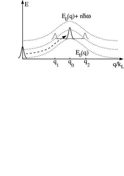
Figure 1: Scheme of the collective wavepacket’s motion through the lowest energy band. The dotted lines represent the spectrum of noninteracting atoms in a 1D optical lattice and a transverse harmonic trap. The lowest of these lines corresponds to the lowest energy band of the lattice for atoms in the transverse ground state. The two upper copies of it are transversally excited atoms in the same band. The BEC is initially prepared as a wavepacket around the lower band edge (lower left corner) and is adiabatically moved to the upper band edge with quasimomentum $q_{0}$ (dashed arrow). Around the upper band edge transversally excited resonances occur at quasimomenta $q_{1}$ and $q_{2}$.

Before we can start to derive an effective equation, the ansatz (5) has to be generalized in two aspects. First, since our aim includes to describe the adiabatic Bloch oscillation from the lower to the upper band edge, we cannot assume that the quasimomentum is fixed, but have to admit a time-dependent $q_{0}(t)$. Secondly, we have to take into account transverse resonances which appear if $q_{0}(t)$ is in the vicinity of the upper band edge (see Ref. kmh02 and Fig. 1). Numerical investigations suggest that it is sufficient to include the two nearest resonances only, because all other resonances are negligibly populated. Therefore, the ansatz (5) needs to be modified to

$$\psi({\bf x},t)=\sum_{i}B_{i}(z,t)\varphi_{q_{i}(t)}(z)\chi_{n_{i}}({\bf x}_{\perp}),$$ (6)

where, for our purposes, $i$ runs from 0 to 2, $q_{i}$ denotes the quasimomentum around which each of the three modes is centered, and $n_{i}$ represents the transverse excitation number ($n_{0}=0,n_{1}=n_{2}=2$ since, by symmetry, only even levels can be excited kmh02 ). $B_{i}$ is a slowly varying envelope function for each of the three modes.

To derive an effective equation for the envelopes, we average over the small spatial scale set by the lattice length $L_{a}=\pi/k_{L}$. Following standard methods, we introduce an averaging function $f_{\mbox{{\scriptsize av}}}(z)$ which is slowly varying on the scale of $L_{a}$, has a narrow support whose width corresponds to the resolution of the effective equation, and which is normalized to one, $\int f_{\mbox{{\scriptsize av }}}(z)dz=1$. The width of $f_{\mbox{{\scriptsize av}}}$ should be much smaller than the scale on which the envelopes $B_{i}$ are varying. A function $g(z)$ is then averaged by calculating $\langle\langle g\rangle\rangle(z):=\int dz^{\prime}f_{\mbox{{\scriptsize av}}}(z^{\prime})g(z-z^{\prime})$. With this method, the envelopes can be extracted from the wavefunction by evaluating

$$\int dz^{\prime}f_{\mbox{{\scriptsize av}}}(z^{\prime})\int d^{2}{\bf x}_{\perp}\,\chi_{n_{i}}^{*}({\bf x}_{\perp})\varphi_{q_{i}}^{*}(z-z^{\prime})\psi({\bf x}_{\perp},z-z^{\prime})$$ (7)

$$= \sum_{j}\delta_{n_{i},n_{j}}\int dz^{\prime}f_{\mbox{{\scriptsize av}}}(z^{\prime})B_{j}(z-z^{\prime})\varphi_{q_{i}}^{*}(z-z^{\prime})\varphi_{q_{j}}(z-z^{\prime})$$

$$\approx \sum_{j}B_{j}(z)\delta_{n_{i},n_{j}}\int dz^{\prime}f_{\mbox{{\scriptsize av}}}(z^{\prime})\varphi_{q_{i}}^{*}(z-z^{\prime})\varphi_{q_{j}}(z-z^{\prime}),$$

where we have used that $B_{j}$ is approximately constant over the support of $f_{\mbox{{\scriptsize av}}}$ and where the time dependence, for brevity, is dropped out. The integral in the last line can be evaluated as follows: for $j=i$ the function $|\varphi_{q_{i}}|^{2}$ is periodic with period $L_{a}$. Therefore, $\int_{0}^{L_{a}}|\varphi_{q_{i}}|^{2}dz=L_{a}/L$ since the Bloch functions are normalized ($L$ is the quantization length). Since $f_{\mbox{{\scriptsize av}}}$ is roughly constant on the scale of $L_{a}$, we find, by cutting the integral into bits of length $L_{a}$,

$$\int dz^{\prime\prime}f_{\mbox{{\scriptsize av}}}(z-z^{\prime\prime})|\varphi_{q_{i}}(z^{\prime\prime})|^{2} \approx \sum_{m}f_{\mbox{{\scriptsize av}}}(z-mL_{a})\frac{L_{a}}{L}$$ (8)

$$\approx \frac{1}{L},$$

since the sum is just the discretized expression for a Riemannian integral over $f_{\mbox{{\scriptsize av}}}$ with $dz=L_{a}$. For $j\neq i$, consider first the case that the width $L_{f}$ of $f_{\mbox{{\scriptsize av}}}$ is very large, $L_{f}=L$. Then the integral is simply the scalar product between the two modes and therefore zero unless $q_{j}=q_{i}$. For sufficiently large $L_{f}$, the integral is still approximately zero if $q_{i}$ and $q_{j}$ are not too close to each other, since the product of the Bloch wavefunctions then oscillates rapidly and averages to zero. Assuming that this is the case we find from Eq. (7)

$$\langle\langle\int d^{2}{\bf x}_{\perp}\,\chi_{n_{i}}^{*}\varphi_{q_{i}}^{*}\psi\rangle\rangle(z)=\frac{B_{i}(z)}{L}.$$ (9)

When we apply the same procedure (projecting onto the transverse modes and averaging over the longitudinal part) to the GPE and insert the ansatz (6), we are led to

$$i\hbar\dot{B}_{i} = \hbar\omega_{\perp}(n_{i}+\frac{1}{2})B_{i}+L\sum_{j}\delta_{n_{i},n_{j}}\langle\langle\varphi_{q_{i}}^{*}H_{\|}\varphi_{q_{j}}B_{j}\rangle\rangle$$ (10)

$$+\kappa\sum_{j,k,l}B_{j}^{*}B_{k}B_{l}I^{\|}_{ij;kl}I^{\perp}_{ij;kl}$$

$$+(\dot{q}_{i}-Ma)zB_{i},$$

with the usual interaction mode integrals

$$I^{\|}_{ij;kl} := \int dz\varphi_{q_{i}}^{*}\varphi_{q_{j}}^{*}\varphi_{q_{k}}\varphi_{q_{l}}$$ (11)

$$I^{\perp}_{ij;kl} := \int d^{2}{\bf x}_{\perp}\chi_{n_{i}}^{*}\chi_{n_{j}}^{*}\chi_{n_{k}}\chi_{n_{l}}\;.$$ (12)

A dot denotes the derivative with respect to time. In the derivation of Eq. (10) we have exploited the fact that the averaging over the interaction integrals can be done in much the same way as for Eq. (7): the averaged interaction integrals are again either periodic or rapidly oscillating and therefore do essentially acquire a factor $1/L$, which we have multiplied out in Eq. (10).

The last line in Eq. (10) deserves a comment. The homogeneous potential term $-Maz$ simply survives the averaging procedure and is a direct consequence of the corresponding term in Eq. (2). The term proportional to $\dot{q}_{i}$ arises from the time derivative on the left-hand side of Eq. (2) which includes a term of the form $\dot{q}_{i}(\partial_{q_{i}}\varphi_{q_{i}})B_{i}$. It is not hard to see that, provided the assumption that the wavepacket remains in the lowest energy band holds true, the derivative with respect to the quasi momentum can be approximated by $\partial_{q_{i}}\varphi_{q_{i}}\approx iz\varphi_{q_{i}}$. The term is then of the same form as the homogeneous force and can be averaged in the same way. It is interesting to note that in the case of a simple Bloch oscillation caused by the homogeneous force we have $\dot{q}_{i}=Ma$ so that the linear potential is cancelled. This is nothing but a different description of the fact that a Bloch oscillation simply corresponds to a shift of a wavepacket in quasimomentum space, again under the condition that no higher bands are populated. This is the case for the main wavepacket in Fig. 1 for which the time dependence of its quasimomentum $q_{0}$ is simply a consequence of the induced Bloch oscillation. However, for the modes $q_{1}$ and $q_{2}$ the time dependence of the quasimomenta is determined by a resonance condition and is not directly related to the Bloch oscillation. Hence, these two modes are subject to a renormalized homogeneous force.

To perform the averaging over the longitudinal Hamiltonian in Eq. (10), we employ the well-known effective-mass method from solid state theory (see, e.g., Ref. hakenQFT ). Using that $B_{j}\varphi_{q_{j}}$ is narrowly localized around quasi momentum $q_{i}$ we can expand this expression in terms of Bloch wave functions $\varphi_{q_{j}+\Delta q}$ , which are eigenfunctions of $H_{\|}$ with eigenvalues $E(q_{j}+\Delta q)$. The eigenvalue can be expanded to second order in $\Delta q$, resulting in

$$H_{\|}\varphi_{q_{j}}B_{j} \approx \int d\Delta q\;\langle\varphi_{q_{j}+\Delta q}|\varphi_{q_{j}}B_{j}\rangle\times$$

$$\left(E(q_{j})+v_{j}\Delta q+\frac{\Delta q^{2}}{2M^{\mbox{{\scriptsize eff}}}_{j}}\right)\varphi_{q_{j}+\Delta q}\;.$$

In this equation, we introduced two important physical parameters: the group velocity $v_{j}:=\partial E(q)/\partial q|_{q=q_{j}}$ and the effective mass $M^{\mbox{{\scriptsize eff}}}_{j}:=(\partial^{2}E(q)/\partial q^{2}|_{q=q_{j}})^{-1}$. Introducing the function

$$\tilde{B}_{j}(z):=\int d\Delta qe^{i\Delta qz}\langle\varphi_{q_{j}+\Delta q}|\varphi_{q_{j}}B_{j}\rangle,$$ (14)

it is easy to see that the action of $H_{\|}$ can be expressed as

$$(H_{\|}\varphi_{q_{j}}B_{j})(z) \approx \int\frac{dz^{\prime}}{2\pi}(H_{\mbox{{\scriptsize eff}},\|}^{(j)}\tilde{B}_{j})(z^{\prime})\times$$ (15)

$$\int d\Delta qe^{-i\Delta qz^{\prime}}\varphi_{q_{j}+\Delta q}(z),$$

with the effective Hamiltonian

$$H_{\mbox{{\scriptsize eff}},\|}^{(j)}=E(q_{j})-i\hbar v_{j}\partial_{z}-\frac{\hbar^{2}\partial_{z}^{2}}{2M^{\mbox{{\scriptsize eff}}}_{j}}\;.$$ (16)

This allows us to write the averaged Hamiltonian action appearing in Eq. (10) in the form

$$\langle\langle\varphi_{q_{i}}^{*}H_{\|}\varphi_{q_{j}}B_{j}\rangle\rangle = \int\frac{dz^{\prime}}{2\pi}(H_{\mbox{{\scriptsize eff}},\|}^{(j)}\tilde{B}_{j})(z^{\prime})\int dz^{\prime\prime}f_{\mbox{{\scriptsize av}}}(z^{\prime\prime})\times$$ (17)

$$\int d\Delta q\;e^{i\Delta q(z-z^{\prime}-z^{\prime\prime})}u_{q_{i}}^{*}(z-z^{\prime\prime})\times$$

$$\hskip 42.67912ptu_{q_{j}+\Delta q}(z-z^{\prime\prime}),$$

where $u_{q}$ are the periodic Bloch wavefunctions, $\varphi_{q}(z)=\exp(iqz)u_{q}(z)$. Because of the averaging, we are interested in distances $z-z^{\prime}$ much larger than $L_{a}$. In this case, the phase factor in the integral over $\Delta q$ varies much faster with $\Delta q$ than the periodic Bloch function $u_{q_{j}+\Delta q}$. We therefore can replace the latter by $u_{q_{j}}$. The integral over $\Delta q$ then becomes, on scales much larger than $L_{a}$, the delta function $2\pi\delta(z-z^{\prime}-z^{\prime\prime})$ and we arrive at

$$\langle\langle\varphi_{q_{i}}^{*}H_{\|}\varphi_{q_{j}}B_{j}\rangle\rangle = \int dz^{\prime\prime}(H_{\mbox{{\scriptsize eff}},\|}^{(j)}\tilde{B}_{j})(z-z^{\prime\prime})f(z^{\prime\prime})\times$$ (18)

$$\varphi_{q_{i}}^{*}(z^{\prime\prime})\varphi_{q_{j}}(z^{\prime\prime})$$

$$\approx (H_{\mbox{{\scriptsize eff}},\|}^{(j)}\tilde{B}_{j})(z)\int dz^{\prime\prime}f(z^{\prime\prime})\times$$

$$\varphi_{q_{i}}^{*}(z^{\prime\prime})\varphi_{q_{j}}(z^{\prime\prime})$$

$$\approx \delta_{q_{i},q_{j}}\frac{1}{L}H_{\mbox{{\scriptsize eff}},\|}^{(j)}\tilde{B}_{j}\;.$$

The last step in our derivation of effective equations for the envelope functions $B_{j}$ is to show that $B_{i}$ and $\tilde{B}_{i}$ are, on average, equal. To do so, we first note that $B_{i}=L\langle\langle\varphi_{q_{i}}^{*}\varphi_{q_{i}}B_{i}\rangle\rangle$ since $B_{i}$ is slowly varying. Inverting Eq.(14), we can rewrite this as

$$B_{i}(z) = L\int dz^{\prime\prime}f_{\mbox{{\scriptsize av}}}(z^{\prime\prime})\int d\Delta q\varphi_{q_{i}}^{*}(z-z^{\prime\prime})\times$$ (19)

$$\varphi_{q_{i}+\Delta q}(z-z^{\prime\prime})\int\frac{dz^{\prime}}{2\pi}e^{-i\Delta qz^{\prime}}\tilde{B}_{i}(z^{\prime})\;.$$

It is then possible to repeat the argument given above for the action of $H_{\|}$. Writing the quasiperiodic Bloch functions $\varphi_{q}$ in terms of the periodic Bloch functions $u_{q}$, we again find a rapidly oscillating exponential in $\Delta q$ which results in a spatial delta function for large scales. Integrating this we find

$$L\langle\langle|\varphi_{q_{i}}|^{2}B_{i}\rangle\rangle = L\langle\langle\tilde{B}_{i}|u_{q_{i}}|^{2}\rangle\rangle$$ (20)

$$\approx L\tilde{B}_{i}\langle\langle|u_{q_{i}}|^{2}\rangle\rangle$$

$$= \tilde{B}_{i}.$$

Using this identity we find for the effective equation describing the large scale dynamics of the envelopes

$$i\hbar\dot{B}_{i} = \hbar\omega_{\perp}(n_{i}+\frac{1}{2})B_{i}+H_{\mbox{{\scriptsize eff}},\|}^{(i)}B_{i}$$ (21)

$$+\kappa\sum_{j,k,l}B_{j}^{*}B_{k}B_{l}I^{\|}_{ij;kl}I^{\perp}_{ij;kl}$$

$$+(\dot{q}_{i}-Ma)zB_{i}\;.$$

For the case of a single wave packet centered around a fixed quasimomentum, an equation similar to Eq. (21) has also been derived using multiple-scale perturbation theory in the context of nonlinear optics sipe88 and atom optics lenz94 ; steel98 ; kon01 . We have chosen a different approach since the inclusion of time-dependent quasi momenta is more obvious using the averaging method. In the following sections we will apply this equation to examine the conditions under which gap solitons can be formed and how they evolve in time.

IV Derivation of variational equations

A major advantage of Eq. (21), compared to the full GPE, is the simple form of the effective Hamiltonians $H_{\mbox{{\scriptsize eff}},\|}^{(i)}$. It describes interacting particles in a homogeneous external potential with different masses and velocities. This allows us to find a simplified analytical description and thus to gain more insight in the dynamics of a BEC in an optical lattice. Numerical simulations of the full GPE indicate that for each mode the wavepacket remains localized around $q_{i}$ for a long time if the optical lattice is not too deep. It is therefore reasonable to assume that the wavepackets can approximately be described as Gaussian wavepackets and to make a variational ansatz for them. Following the technique described in Refs. orgcit2 ; perez96 , we first observe that Eq. (21) can formally be derived from the Lagrangean

$${\cal L} = \sum_{i}\Big{\{}i\frac{\hbar}{2}\left(\dot{B}_{i}^{*}B_{i}-B_{i}^{*}\dot{B}_{i}\right)$$ (22)

$$+\left(E(q_{i})+\hbar\omega_{\perp}(n_{i}+\frac{1}{2})-(Ma-\dot{q}_{i})z\right)|B_{i}|^{2}$$

$$+i\frac{\hbar v_{i}}{2}\left(\partial_{z}B_{i}^{*}B_{i}-B_{i}^{*}\partial_{z}B_{i}\right)+\frac{\hbar^{2}}{2M^{\mbox{{\scriptsize eff}}}_{i}}|\partial_{z}B_{i}|^{2}\Big{\}}$$

$$+\frac{\kappa}{2}\sum_{i,j,k,l}B_{i}^{*}B_{j}^{*}B_{k}B_{l}I^{\|}_{ij;kl}I^{\perp}_{ij;kl}.$$

A consistent variational ansatz for Gaussian envelopes is achieved by setting

$$B_{i}(z,t) = \frac{A_{i}(t)}{\sqrt{\pi^{1/2}w_{i}(t)}}\exp\Big{(}-\frac{(z-z_{i}(t))^{2}}{2w_{i}(t)^{2}}-i\phi_{i}(t)$$ (23)

$$\hskip 28.45274pt+i\beta_{i}(t)z+i\gamma_{i}(t)z^{2}\Big{)}.$$

This describes a wavepacket of width $w_{i}$ and amplitude $A_{i}$ (having dimensions of length^1/2 so that $B_{i}$ is dimensionless). It is spatially localized around $z_{i}$ and has an instantaneous energy of $\hbar\dot{\phi}_{i}$. Its mean velocity and its variance are given by $\langle v_{i}\rangle=(\beta_{i}+2\gamma_{i}w_{i})/M_{i}^{\mbox{{\scriptsize eff}}}$ and $\Delta v_{i}=\sqrt{2\gamma_{i}^{2}w_{i}^{2}+1/(2w_{i}^{2})}/M_{i}^{\mbox{{\scriptsize eff}}}$.

Inserting this ansatz for the envelopes in the Lagrangean and extremizing the corresponding action integral, we derived a set of 18 equations which describe the evolution of the three Gaussian wavepackets involved. This task, as well as the algebraic manipulations following below, are rather tedious and therefore have been completed using Mathematica Mathematica . Since the variational equations are somewhat lengthy we exploited the special features of our system to reduce its complexity. To do so, we restrict our considerations to the case when the wavepackets are already at the upper band edge so that the quasi momenta are time-independent and given by $q_{0}=\hbar k_{L}$ and $q_{1}=\hbar k_{L}-\delta q$ as well as $q_{2}=\hbar k_{L}+\delta q$, where $k_{L}$ is the wavenumber of the optical lattice which appears in the optical potential (1). $\delta q$ is identical to $q_{2}-q_{0}$. It can be derived from the resonance condition that the three energies $E(q_{i})+\hbar\omega_{\perp}(n_{i}+\frac{1}{2})$ for $i=0,1,2$ are equal. Setting this energy to zero we can also omit the corresponding terms in the Lagrangean. Because the wavepackets are already at the upper band edge we will also not need the homogeneous force to induce Bloch oscillations, i.e., we set $a=\dot{q}_{i}=0$.

The special values of the quasi momenta imply that most of the interaction integrals $I^{\|}_{ij;kl}$ are zero or have an identical value. This can be seen by expanding the Bloch wavefunctions in terms of momentum eigenstates, $\varphi_{q}(z)=\sum_{l}c_{l}(q)\exp(iz(q+2l\hbar k_{L}))$. By Fourier transforming the stationary Schrödinger equation $H_{\|}\varphi_{q}=E(q)\varphi_{q}$, one finds the following equation for the expansion coefficients $c_{l}(q)$,

$$E(q)c_{l}(q)=\frac{(q+2l\hbar k_{L})^{2}}{2M}c_{l}(q)+\frac{V_{0}}{2}\big{(}c_{l+1}(q)+c_{l-1}(q)\big{)}.$$ (24)

This equation shows that the expansion coefficients are real and that, if $c_{l}(\hbar k_{L}-\delta q)$ is a solution, then so is $c_{l}(\hbar k_{L}+\delta q)=c_{-l-1}(\hbar k_{L}-\delta q)$. Thus, we have the relation

$$\varphi_{q_{2}}(z)=\varphi_{q_{1}}^{*}(z)\;.$$ (25)

It is well known, and can be seen from the above expansion, that Bloch wavefunctions are periodic up to a phase factor $\exp(iqx)$. Therefore, the three wavefunctions $\varphi_{q_{i}}$ are oscillating with a phase factor $\exp(\pm i\delta qx)$ relative to each other. In the limit of an infinite optical lattice, the interaction integral $I^{\|}_{ij;kl}$ will therefore vanish if these phase factors do not exactly cancel each other. For instance, $I^{\|}_{00;01}=0$ because its integrand is proportional to $\exp(i\delta qx)$, but $I^{\|}_{00;12}\neq 0$. This, in combination with Eq. (25), ensures that all interaction integrals, except $I^{\|}_{00;00}$ and $I^{\|}_{11;11}=I^{\|}_{22;22}=I^{\|}_{12;12}$ as well as $I^{\|}_{01;01}=I^{\|}_{02;02}=I^{\|}_{00;12}$, do vanish (in addition, the symmetries $I^{\|}_{ij;kl}=I^{\|}_{ji;kl}$ and $I^{\|}_{ij;lk}=I^{\|}_{ij;kl}$ have to be taken into account). Thus, there are only three independent interaction parameters which we will denote by

$$\kappa_{0} := \frac{\kappa}{\sqrt{\pi}\hbar}I^{\|}_{00;00}I^{\perp}_{00;00}\;,$$

$$\kappa_{1} := \frac{\kappa}{\sqrt{\pi}\hbar}I^{\|}_{11;11}I^{\perp}_{11;11}\;,$$

$$\kappa_{01} := \frac{\kappa}{\sqrt{\pi}\hbar}I^{\|}_{01;01}I^{\perp}_{01;01}\;.$$ (26)

Even with these simplifications the resulting equations are still very lengthy, but they admit the analysis of symmetric solutions. By symmetry, we have $v_{0}=0$ and $v_{2}=-v_{1}$ for the group velocities of the wavepacket, and $M^{\mbox{{\scriptsize eff}}}_{2}=M^{\mbox{{\scriptsize eff}}}_{1}$ for the effective masses. Under these conditions one can show that $z_{0}=0$ and $\beta_{0}=0$ are solutions of the variational equations. This result is intuitively clear and just means that the central wavepacket remains at the upper band edge with mean position and velocity zero. In addition, symmetry implies that the two transversally excited wavepackets should evolve in an identical way, but with opposite mean velocities (because their group velocities differ by a sign). We therefore can set $A_{2}=A_{1}$, $\gamma_{2}=\gamma_{1}$, $\phi_{2}=\phi_{1}$, $w_{2}=w_{1}$, and $\beta_{2}=-\beta_{1}$, $z_{2}=-z_{1}$, which reduces the number of independent variational parameters to ten (four for $q_{0}$ and six for $q_{1}$). In addition, the conservation of the number of atoms implies the constraint $A_{0}^{2}+2A_{1}^{2}=L$, so that we are effectively left with nine independent parameters . The resulting variational equations are given by

$$\dot{A}_{0}=\frac{e^{-\frac{z_{1}^{2}}{w_{1}^{2}}}\,S^{(1)}\,{A_{0}}\,{{A_{1}}}^{2}\,{{\kappa}_{01}}}{{w_{0}}{w_{1}}},$$ (27)

$$\dot{z}_{1}={v_{1}}+\frac{\hbar\,{{\beta}_{1}}}{{M^{\mbox{{\scriptsize eff}}}_{1}}}+\frac{2\,\hbar\,{z_{1}}\,{{\gamma}_{1}}}{{M^{\mbox{{\scriptsize eff}}}_{1}}}+\frac{e^{-\frac{z_{1}^{2}}{w_{1}^{2}}}\,S^{(1)}\,{{A_{0}}}^{2}\,{z_{1}}\,{{\kappa}_{01}}}{{w_{0}}\,{w_{1}}},$$ (28)

$$\dot{w}_{0}=\frac{2\,\hbar\,{w_{0}}\,{{\gamma}_{0}}}{{M^{\mbox{{\scriptsize eff}}}_{0}}}+\frac{e^{-\frac{z_{1}^{2}}{w_{1}^{2}}}\,{{A_{1}}}^{2}\,\left(S^{(3)}-S^{(1)}\,{{w_{0}}}^{2}\right)\,{{\kappa}_{01}}}{{{w_{0}}}^{2}\,{w_{1}}},$$ (29)

$$\dot{w}_{1} = \frac{2\,\hbar\,{w_{1}}\,{{\gamma}_{1}}}{{M^{\mbox{{\scriptsize eff}}}_{1}}}+$$

$$\frac{e^{-\frac{z_{1}^{2}}{w_{1}^{2}}}\,{{A_{0}}}^{2}\,\left(-S^{(3)}+S^{(1)}\,{{w_{1}}}^{2}-2\,S^{(1)}\,{{z_{1}}}^{2}\right)\,{{\kappa}_{01}}}{2{w_{0}}\,{{w_{1}}}^{2}},$$

$$\dot{\gamma}_{0} = \frac{\hbar}{2\,{M^{\mbox{{\scriptsize eff}}}_{0}}\,{{w_{0}}}^{4}}-\frac{2\,\hbar\,{{{\gamma}_{0}}}^{2}}{{M^{\mbox{{\scriptsize eff}}}_{0}}}+\frac{{{A_{0}}}^{2}\,{{\kappa}_{0}}}{2\,{\sqrt{2}}{{w_{0}}}^{3}}+$$

$$\frac{e^{-\frac{z_{1}^{2}}{w_{1}^{2}}}\,{{A_{1}}}^{2}\,\left(-C^{(3)}+C^{(1)}\,{{w_{0}}}^{2}\right)\,{{\kappa}_{01}}}{{{w_{0}}}^{5}\,{w_{1}}}+$$

$$\frac{4\,e^{-\frac{z_{1}^{2}}{\bar{w}^{2}}}\,{{A_{1}}}^{2}\,\left({\bar{w}}^{2}-2\,{{z_{1}}}^{2}\right)\,{{\kappa}_{01}}}{{\bar{w}}^{5}},$$

$$\dot{\gamma}_{1} = \frac{\hbar}{2\,{M^{\mbox{{\scriptsize eff}}}_{1}}\,{{w_{1}}}^{4}}-\frac{2\,\hbar\,{{{\gamma}_{1}}}^{2}}{{M^{\mbox{{\scriptsize eff}}}_{1}}}+\frac{{{A_{1}}}^{2}\,{{\kappa}_{1}}}{2\,{\sqrt{2}}{{w_{1}}}^{3}}+$$

$$\frac{{e^{-2\frac{z_{1}^{2}}{w_{1}^{2}}}}\,{{A_{1}}}^{2}\,\left({{w_{1}}}^{2}-4\,{{z_{1}}}^{2}\right)\,{{\kappa}_{1}}}{{\sqrt{2}}{{w_{1}}}^{5}}+$$

$$\frac{2{{\kappa}_{01}}\,e^{-\frac{z_{1}^{2}}{\bar{w}^{2}}}\,{{A_{0}}}^{2}\,\left({\bar{w}}^{2}-2\,{{z_{1}}}^{2}\right)}{{\bar{w}}^{5}}+$$

$$\frac{{{\kappa}_{01}}e^{-\frac{z_{1}^{2}}{w_{1}^{2}}}\,{{A_{0}}}^{2}\,\left(-C^{(3)}+C^{(1)}({{w_{1}}}^{2}-2{{z_{1}}}^{2})\right)}{2\,{w_{0}}\,{{w_{1}}}^{5}},$$

$$\dot{\phi}_{0} = \frac{\hbar}{2\,{M^{\mbox{{\scriptsize eff}}}_{0}}\,{{w_{0}}}^{2}}+\frac{5\,{{A_{0}}}^{2}\,{{\kappa}_{0}}}{4\,{\sqrt{2}}{w_{0}}}+$$

$$\frac{e^{-\frac{z_{1}^{2}}{w_{1}^{2}}}\,{{A_{1}}}^{2}\,\left(-C^{(3)}+3\,C^{(1)}\,{{w_{0}}}^{2}\right)\,{{\kappa}_{01}}}{2\,{{w_{0}}}^{3}\,{w_{1}}}+$$

$$\frac{2\,e^{-\frac{z_{1}^{2}}{\bar{w}^{2}}}\,{{A_{1}}}^{2}\,\left(3\,{{w_{0}}}^{4}+2\,{{w_{1}}}^{4}+{{w_{0}}}^{2}\,\left(5\,{{w_{1}}}^{2}-2\,{{z_{1}}}^{2}\right)\right)\,{{\kappa}_{01}}}{{\bar{w}}^{5}},$$

$$\dot{\phi}_{1} = \frac{\hbar}{2\,{M^{\mbox{{\scriptsize eff}}}_{1}}\,{{w_{1}}}^{2}}-\frac{\hbar\,{{z_{1}}}^{2}}{2\,{M^{\mbox{{\scriptsize eff}}}_{1}}\,{{w_{1}}}^{4}}+{v_{1}}\,{{\beta}_{1}}+$$

$$\frac{\hbar\,{{{\beta}_{1}}}^{2}}{2\,{M^{\mbox{{\scriptsize eff}}}_{1}}}+\frac{{{\kappa}_{2}}{{A_{1}}}^{2}}{4\,{\sqrt{2}}{{w_{1}}}^{5}}\Big{(}5\,\big{(}1+2\,{e^{-2\frac{z_{1}^{2}}{w_{1}^{2}}}}\big{)}\,{{w_{1}}}^{4}+$$

$$\hskip 28.45274pt2\,\big{(}-1+2\,{e^{-2\frac{z_{1}^{2}}{w_{1}^{2}}}}\big{)}\,{{w_{1}}}^{2}\,{{z_{1}}}^{2}+16\,{e^{-2\frac{z_{1}^{2}}{w_{1}^{2}}}}\,{{z_{1}}}^{4}\Big{)}\,+$$

$$\frac{e^{-\frac{z_{1}^{2}}{w_{1}^{2}}}\,{{A_{0}}}^{2}{{\kappa}_{01}}}{4{w_{0}}\,{{w_{1}}}^{5}}\big{(}C^{(3)}(2{{z_{1}}}^{2}-{{w_{1}}}^{2})+$$

$$\hskip 28.45274ptC^{(1)}(3{{w_{1}}}^{4}+4{{z_{1}}}^{4})\big{)}+$$

$$\frac{e^{-\frac{z_{1}^{2}}{\bar{w}^{2}}}\,{{A_{0}}}^{2}{{\kappa}_{01}}}{{\bar{w}}^{5}}\big{(}2\,{{w_{0}}}^{4}+3\,{{w_{1}}}^{4}+4\,{{z_{1}}}^{4}+$$

$$\hskip 28.45274pt{{w_{0}}}^{2}\,\left(5\,{{w_{1}}}^{2}+2\,{{z_{1}}}^{2}\big{)}\right),$$

$$\dot{\beta}_{1} = -\frac{\hbar\,{z_{1}}}{{M^{\mbox{{\scriptsize eff}}}_{1}}\,{{w_{1}}}^{4}}-2\,{v_{1}}\,{{\gamma}_{1}}-\frac{2\,\hbar\,{{\beta}_{1}}\,{{\gamma}_{1}}}{{M^{\mbox{{\scriptsize eff}}}_{1}}}+$$

$$\frac{{e^{-2\frac{z_{1}^{2}}{w_{1}^{2}}}}\,{\sqrt{2}}\,{{A_{1}}}^{2}\,{z_{1}}\,\left({{w_{1}}}^{2}+4\,{{z_{1}}}^{2}\right)\,{{\kappa}_{1}}}{{{w_{1}}}^{5}}-\frac{{{A_{1}}}^{2}\,{z_{1}}\,{{\kappa}_{1}}}{{\sqrt{2}}{{w_{1}}}^{3}}+$$

$$\frac{8\,e^{-\frac{z_{1}^{2}}{\bar{w}^{2}}}\,{{A_{1}}}^{2}\,{{z_{1}}}^{3}\,{{\kappa}_{01}}}{{\bar{w}}^{5}}+$$

$$\frac{e^{-\frac{z_{1}^{2}}{w_{1}^{2}}}\,{{A_{0}}}^{2}\,{z_{1}}\,\left(C^{(3)}+2\,C^{(1)}\,{{z_{1}}}^{2}\right)\,{{\kappa}_{01}}}{{w_{0}}\,{{w_{1}}}^{5}}.$$

In these equations we have introduced the notation $\bar{w}:=\sqrt{w_{0}^{2}+w_{1}^{2}}$ and

$$S^{(n)} := i\frac{e^{-2i(\phi_{0}-\phi_{1})}}{\left(\frac{1}{w_{0}^{2}}+\frac{1}{w_{1}^{2}}-2i(\gamma_{0}-\gamma_{1})\right)^{n/2}}+c.c.\;,$$

$$C^{(n)} := \frac{e^{-2i(\phi_{0}-\phi_{1})}}{\left(\frac{1}{w_{0}^{2}}+\frac{1}{w_{1}^{2}}-2i(\gamma_{0}-\gamma_{1})\right)^{n/2}}+c.c.\;.$$ (36)

The functions $S^{(n)}$ depend on $\phi_{i}$, $\gamma_{i}$, and $w_{i}$ and do vanish for $\phi_{1}-\phi_{0}=0$.

V Special solutions of the variational equations

Initially empty transverse excited modes: A surprising consequence of the variational equations can be seen immediately: it follows from Eq. (27) that, when all atoms are in the central wavepacket ($A_{1}=0$), the amplitude $A_{0}$ and therefore also $A_{1}$ will not change in time. Thus, the transversally excited wavepackets would never be populated. This prediction is a direct consequence of the assumption $I^{\|}_{00;01}\;(=I^{\|}_{00;02})\;=0$ and in striking contradiction to the numerical results of Ref. kmh02 . This difference can be resolved when one recalls the conditions under which our analytical theory is valid. $I^{\|}_{00;01}=0$ is exactly fullfilled only in the limit of an infinite optical lattice. In a finite lattice the fact (discussed above) that the integrand is oscillating with a phase factor of $\exp(\pm i\delta qz)$ only leads to oscillations of $I^{\|}_{00;01}$, so that it is zero on average only. Since our wavepackets have a finite width in quasimomentum space, there will be a finite excitation probability even when $A_{1}=0$ initially. In addition, our theory assumes that the three wavepackets are not overlapping in quasimomentum space, since only under this condition the averaging method can yield reasonable results. In practice, this is not exactly fulfilled and will lead to corrections to the prediction of the averaged equations. However, the time scale for transverse excitation out of a central wavepacket is quite large (typically about 70 ms kmh02 ) so that the averaged equations should provide a valid description for shorter times. In fact, the present considerations may provide another reason for the long time scales for transverse excitations. In addition, during the preparation of the wavepacket at the upper band edge through Bloch oscillations, the transversally excited modes are populated. Therefore, an initial condition with $A_{1}(0)\neq 0$ is realistic when we describe a system that already is prepared at the upper band edge.

On the other hand, when using the initial condition $A_{1}(0)=0$ we are left with a theory for the central wavepacket only, since there are never any transversally excited atoms to interact with. In this case our description reduces to the case considered in Ref. perez96 (but with a negative effective mass) so that one can transfer most of the results to our case. We therefore will not discuss it further.

Case of three initial gap solitons: Another case of interest is the case when all three wavepackets are initially forming independent gap solitons. That is, in the absence of mutual interactions each of the three envelopes corresponds to a stationary solution of the variational equations with self-interaction. We can find these solutions by setting $\kappa_{01}=0$ and removing the terms proportional to $\kappa_{1}\exp(-2z_{1}^{2}/w_{1}^{2})$, which describe the interaction between wavepacket $q_{1}$ and $q_{2}$ (see above). It is easy to see that in this case the soliton solution is given by $\gamma_{i}=\beta_{i}=0$ and $z_{1}^{\mbox{{\scriptsize sol}}}=v_{1}t$ as well as

$$w_{i}^{\mbox{{\scriptsize sol}}} = -\frac{\sqrt{2}\hbar}{{A^{\mbox{{\scriptsize sol}}}_{i}}^{2}\kappa_{i}M^{\mbox{{\scriptsize eff}}}_{i}},$$ (37)

$$\phi_{i}^{\mbox{{\scriptsize sol}}} = \phi_{i}(0)+\frac{3{A^{\mbox{{\scriptsize sol}}}_{i}}^{2}\kappa_{i}}{4\sqrt{2}\;w_{i}^{\mbox{{\scriptsize sol}}}}t\;.$$ (38)

The question remains whether this solution is stable against the presence of the mutual interactions of the three gap solitions. To answer it, we have made a stability analysis by linearizing the variational equations in the deviations from the soliton solution (37), (38). We set $w_{i}=w_{i}^{\mbox{{\scriptsize sol}}}+\epsilon\delta w_{i}$ (and similarly for the other dynamical variables) and consider all equations only to first order in $\epsilon$, whereby the mutual interaction terms are treated as of first order in $\epsilon$. This is justified since these terms all include a factor which exponentially decays in time and thus have limited influence. Such a factor arises because the three wavepackets all have different group velocities and thus separate after a short time, the exponential being a consequence of the overlap between the Gaussian wavepackets. The resulting linearized equations are given by

$$\dot{\delta A}_{0}=e^{-\big{(}\frac{t\,v_{1}}{w_{1}^{\mbox{{\scriptsize sol}}}}\big{)}^{2}}\frac{2\,\sin(\Delta\phi)\,A_{0}^{\mbox{{\scriptsize sol}}}\,{A_{1}^{\mbox{{\scriptsize sol}}}}^{2}\,{{\kappa}_{01}}}{w_{1}^{\mbox{{\scriptsize sol}}}},$$ (39)

$$\dot{\delta w}_{0}=-{\sqrt{2}}\,{A_{0}^{\mbox{{\scriptsize sol}}}}^{2}\,\delta\gamma_{0}\,{{\kappa}_{0}}\,{w_{0}^{\mbox{{\scriptsize sol}}}}^{2},$$ (40)

$$\dot{\delta\gamma}_{0}=\frac{{A_{0}^{\mbox{{\scriptsize sol}}}}^{2}\,\delta w_{0}\,{{\kappa}_{0}}}{2\,{\sqrt{2}}\,{w_{0}^{\mbox{{\scriptsize sol}}}}^{4}}+\frac{A_{0}^{\mbox{{\scriptsize sol}}}\,\delta A_{0}\,{{\kappa}_{0}}}{{\sqrt{2}}\,{w_{0}^{\mbox{{\scriptsize sol}}}}^{3}}+e^{-\big{(}\frac{t\,v_{1}}{w_{1}^{\mbox{{\scriptsize sol}}}}\big{)}^{2}}f_{\gamma_{0}}(t),$$ (41)

$$\dot{\delta\phi}_{0}=\frac{-{A_{0}^{\mbox{{\scriptsize sol}}}}^{2}\,\delta w_{0}\,{{\kappa}_{0}}}{4\,{\sqrt{2}}\,{w_{0}^{\mbox{{\scriptsize sol}}}}^{2}}+\frac{5\,A_{0}^{\mbox{{\scriptsize sol}}}\,\delta A_{0}\,{{\kappa}_{0}}}{2\,{\sqrt{2}}\,w_{0}^{\mbox{{\scriptsize sol}}}}+e^{-\big{(}\frac{t\,v_{1}}{w_{1}^{\mbox{{\scriptsize sol}}}}\big{)}^{2}}f_{\phi_{0}}(t),$$ (42)

$$\dot{\delta z}_{1}=-\frac{{A_{1}^{\mbox{{\scriptsize sol}}}}^{2}\,\left(\delta\beta_{1}+2\,t\,{v_{1}}\,\delta\gamma_{1}\right)\,{{\kappa}_{1}}\,w_{1}^{\mbox{{\scriptsize sol}}}}{{\sqrt{2}}}+e^{-\big{(}\frac{t\,v_{1}}{w_{1}^{\mbox{{\scriptsize sol}}}}\big{)}^{2}}f_{z_{1}}(t),$$ (43)

$$\dot{\delta w}_{1}=-{\sqrt{2}}\,{A_{1}^{\mbox{{\scriptsize sol}}}}^{2}\,\delta\gamma_{1}\,{{\kappa}_{1}}\,{w_{1}^{\mbox{{\scriptsize sol}}}}^{2}+e^{-\big{(}\frac{t\,v_{1}}{w_{1}^{\mbox{{\scriptsize sol}}}}\big{)}^{2}}f_{w_{1}}(t),$$ (44)

$$\dot{\delta\beta}_{1} = -\frac{{{\kappa}_{1}}\,{v_{1}}t\,\left(\,{A_{1}^{\mbox{{\scriptsize sol}}}}^{2}\,\delta w_{1}\,+2\,A_{1}^{\mbox{{\scriptsize sol}}}\,\delta A_{1}\,\,w_{1}^{\mbox{{\scriptsize sol}}}\right)}{\sqrt{2}\,{w_{1}^{\mbox{{\scriptsize sol}}}}^{4}}$$ (45)

$$-2v_{1}\delta\gamma_{1}+e^{-\big{(}\frac{t\,v_{1}}{w_{1}^{\mbox{{\scriptsize sol}}}}\big{)}^{2}}f_{\beta_{1}}(t),$$

$$\dot{\delta\gamma}_{1}=\frac{A_{1}^{\mbox{{\scriptsize sol}}}\,{{\kappa}_{1}}\,\left(A_{1}^{\mbox{{\scriptsize sol}}}\,\delta w_{1}+2\,\delta A_{1}\,w_{1}^{\mbox{{\scriptsize sol}}}\right)}{2\,{\sqrt{2}}\,{w_{1}^{\mbox{{\scriptsize sol}}}}^{4}}+e^{-\big{(}\frac{t\,v_{1}}{w_{1}^{\mbox{{\scriptsize sol}}}}\big{)}^{2}}f_{\gamma_{1}}(t),$$ (46)

$$\dot{\delta\phi}_{1} = -\frac{{A_{1}^{\mbox{{\scriptsize sol}}}}^{2}\,\delta w_{1}\,{{\kappa}_{1}}\,\left(2\,t^{2}\,{{v_{1}}}^{2}+{w_{1}^{\mbox{{\scriptsize sol}}}}^{2}\right)}{4\sqrt{2}\,{w_{1}^{\mbox{{\scriptsize sol}}}}^{4}}$$ (47)

$$+\frac{A_{1}^{\mbox{{\scriptsize sol}}}\,\delta A_{1}\,{{\kappa}_{1}}\,\left(-2\,t^{2}\,{{v_{1}}}^{2}+5\,{w_{1}^{\mbox{{\scriptsize sol}}}}^{2}\right)}{2\,{\sqrt{2}}\,{w_{1}^{\mbox{{\scriptsize sol}}}}^{3}}$$

$$+{v_{1}}\,\delta\beta_{1}\,+e^{-\big{(}\frac{t\,v_{1}}{w_{1}^{\mbox{{\scriptsize sol}}}}\big{)}^{2}}f_{\phi_{1}}(t).$$

The functions $f_{\alpha}(t)$ depend on the soliton solution parameters and increase at most polynomially (degree less than 4) in time. They represent inhomogenities, similarly to the right-hand side of Eq. (39). Because of the exponentially decaying factor, these terms are only important for times $t<w_{1}^{\mbox{{\scriptsize sol}}}/v_{1}$. Therefore, to analyze the stability of the soliton solution, it is sufficient to solve the homogeneous linearized equations for a general set of initial conditions, since for large enough times this correctly describes the general solution.

To reduce the length of the linearized equations we have made an additional approximation. Our numerical simulations of the full GPE indicate that, after the BEC has been transferred to the upper band edge, the number of atoms in the $q_{0}$ wavepacket is considerably larger than in the other two modes . Since $A_{i}^{2}=LN_{i}$, where $N_{i}$ is the initial number of atoms in each mode, one can see that $A_{1}^{\mbox{{\scriptsize sol}}}\ll A_{0}^{\mbox{{\scriptsize sol}}}$ and therefore $w_{1}^{\mbox{{\scriptsize sol}}}\gg w_{0}^{\mbox{{\scriptsize sol}}}$. Assuming that this is the case, we here present the linearized equations only to second order in the ratio $A_{1}^{\mbox{{\scriptsize sol}}}/A_{0}^{\mbox{{\scriptsize sol}}}$.

The general solution of the homogeneous linearized equations is not hard to find. One immediately sees that $\delta A_{0}$ and therefore, because of atom number conservation, also $\delta A_{1}$ are constant in time. $\delta w_{0}$ and $\delta\gamma_{0}$ are then coupled to each other only so that Eqs. (40) and (41) are easily solved. $\delta w_{0}$ and $\delta\gamma_{0}$ then generally show a purely oscillating behaviour. This solution can then be inserted into Eq. (42) for the homogeneous phase factor. The latter then grows in time, in addition to some oscillating factors, proportional to $3t\kappa_{0}A_{0}^{\mbox{{\scriptsize sol}}}\delta A_{0}(0)/(\sqrt{2}w_{0}^{\mbox{{\scriptsize sol}}})$. When this expression is compared to the evolution of the solition phase factor (38) it becomes obvious that this linear increase in $\delta\phi_{0}$ just corresponds to a small deviation, proportional to $\delta A_{0}(0)/A_{0}^{\mbox{{\scriptsize sol}}}$, from the unperturbed energy of the soliton. We therefore have shown that the central soliton around quasi momentum $q_{0}$ is stable against the interaction with the other two wavepackets since its stability does also not depend on the evolution of the deviations in these wavepackets.

The situation is quite different for the transversally excited modes. Repeating the steps leading to the solution for the central wavepacket, one can see that the solution for $\delta\beta_{1}$ is given by

$$\delta\beta_{1}(t) = \delta\beta_{1}(0)-2v_{1}t\cos(\Omega_{1}t){{\delta\gamma}_{1}}(0)$$

$$-\frac{v_{1}t\sin(\Omega_{1}t)}{{w_{1}^{\mbox{{\scriptsize sol}}}}^{2}}\left(2\frac{\delta A_{1}(0)}{A_{1}^{\mbox{{\scriptsize sol}}}}+\frac{\delta w_{1}(0)}{w_{1}^{\mbox{{\scriptsize sol}}}}\right),$$

with $\Omega_{1}:=(4/3)d\phi_{1}^{\mbox{{\scriptsize sol}}}/dt$. This growing oscillatory behaviour clearly indicates instability against any initial deviations $\delta w_{1}(0),\delta A_{1}(0),\delta\gamma_{1}(0)$, which unavoidably are introduced by the interaction between the three wavepackets.

It is worth to examine the origin of this instability more closely. Our arguments are based on the fact that the two transversally excited wavepackets move away from the central wavepacket. This happens because we have set $\beta_{1}=\beta_{2}=0$ for the excited wavepackets, so that they propagate with the group velocity $\pm v_{1}$. Hence, after some time the wavepackets are separated, so that the mutual interaction disappears and cannot cause instability anymore. However, setting $\beta_{i}=0$ in absence of mutual interactions creates another source of instability: even in a strictly one-dimensional situation, a gap (or bright) soliton with non-vanishing group velocity is only stable if the phase factor exactly matches the group velocity, $\beta_{i}=-M_{i}^{\mbox{{\scriptsize eff}}}v_{i}/\hbar$ . Therefore, the instability of the transversally excited wavepackets is the same as that of an isolated gap soliton with the wrong phase factor.

The only possibility to avoid this kind of instability is to choose the appropriate phase factors $\beta_{2}=-\beta_{1}=-M_{1}^{\mbox{{\scriptsize eff}}}v_{1}/\hbar$. As a consequence, the excited wavepackets would remain at their original position so that the mutual interaction would not decrease. Since the latter is a resonant coupling between the three wavepackets a general superposition of three gap solitons would not correspond to a stationary solution anymore. In the next section we will demonstrate that for a particular choice of parameters this problem can be overcome.

VI Triple solitons

A particularly interesting situation appears when one tries to construct stationary wavepackets which remain spatially localized around $z_{1}=0$. As is evident from Eq. (28), this is only possible for $\beta_{1}=-M_{1}^{\mbox{{\scriptsize eff}}}v_{1}/\hbar$. Interestingly, this condition also guarantees the validity of $\dot{\beta}_{1}=0$ in Eq. (IV), so that this requirement is self-consistent. The remaining equations will only lead to a stationary solution if the populations of the three modes are constant, i.e., if $\dot{A}_{0}=0$. Apart from the trivial solutions $A_{0}=0$ or $A_{1}=0$ this can be achieved by the condition $S^{(1)}=0$. A natural solution to this condition is $\phi_{1}-\phi_{0}=0$ and $\gamma_{0}=\gamma_{1}=0$, whereby the latter assumption also ensures that the widths of the wavepackets remain constant. A necessary condition for this to hold are the equations

$$\dot{\phi}_{1}-\dot{\phi}_{0}=\dot{\gamma}_{0}=\dot{\gamma}_{1}=0\;.$$ (49)

Using Eqns. (IV) - (IV) this leads to algebraic conditions on the widths and populations of the three modes. The simplest way to solve these algebraic conditions is to, first, fix the ratio between the widths according to $w_{2}=\eta w_{1}$, where $\eta$ is some positive number. In addition, we write $\kappa_{i}=N\bar{\kappa}_{i}/L$ so that $\bar{\kappa}_{i}$ is independent of the total number of atoms $N$ and remains finite when the quantization length $L$ goes to infinity. For these settings we derived solutions of the algebraic conditions which determine $N$, $w_{1}$, and the population distribution among the modes as a function of $\eta$, $\bar{\kappa}_{i}$, $M_{i}^{\mbox{{\scriptsize eff}}}$, and $v_{1}$. A particularly nice example is the case when all three wavepackets have equal width, $w_{1}=w_{0}$. The solution then becomes very compact and is given by

$$A_{1}^{2} = L\frac{3M^{\mbox{{\scriptsize eff}}}_{1}\bar{\kappa}_{1}-6M^{\mbox{{\scriptsize eff}}}_{0}\bar{\kappa}_{01}}{2M^{\mbox{{\scriptsize eff}}}_{0}(\bar{\kappa}_{0}-3\bar{\kappa}_{01})+3M^{\mbox{{\scriptsize eff}}}_{1}(\bar{\kappa}_{1}-2\bar{\kappa}_{01})},$$ (50)

$$N = \frac{2v_{1}\!\left(2M^{\mbox{{\scriptsize eff}}}_{0}(\frac{\bar{\kappa}_{0}}{3}-\!\bar{\kappa}_{01})+M^{\mbox{{\scriptsize eff}}}_{1}(\bar{\kappa}_{1}-\!2\bar{\kappa}_{01})\right)}{(6\bar{\kappa}_{01}^{2}-\bar{\kappa}_{0}\bar{\kappa}_{1})\sqrt{3M^{\mbox{{\scriptsize eff}}}_{0}(M^{\mbox{{\scriptsize eff}}}_{1}-M^{\mbox{{\scriptsize eff}}}_{0})}},$$ (51)

$$w_{1} = \frac{\hbar}{-{M^{\mbox{{\scriptsize eff}}}_{1}}\,{v_{1}}}\sqrt{\frac{{3({M^{\mbox{{\scriptsize eff}}}_{0}}-{M^{\mbox{{\scriptsize eff}}}_{1}})}}{-2{M^{\mbox{{\scriptsize eff}}}_{0}}}},$$ (52)

with $w_{2}=w_{1}=w_{0}$ and $\bar{\kappa}_{i}:=\kappa_{i}L/N$ being independent from the number of atoms and the quantization length.

The state characterized by Eqs. (50)-(52), which we will refer to as “triple soliton”, represents a special coherent superposition of a wavepacket in the transverse ground state at the upper band edge of the optical lattice, and two wavepackets around the transverse resonances. The special choice (50)-(52) for the parameters ensures that the mutual and self-interaction of the wavepackets exactly cancel the dispersion of each wavepacket due to its negative effective mass. It also guarantees, within the approximation that only two resonances are taken into account, that the triple soliton does not spread in the transverse direction. It therefore can be seen as a generalization of the gap soliton which is unstable against transverse decay. It differs from the case of a superposition of three gap-soliton wavepackets discussed above in that the mutual interaction between the wavepackets destroys the latter. This is because the stability criterion (37) and (38) takes only into account the self-interaction of each of the three wavepackets. For the triple soliton the mutual interaction is included as well.

A very interesting feature of the triple soliton is that the width of the soliton does not depend in any way on the interaction parameters of the system. It is solely determined by the structure of the lowest energy band of the optical lattice and in particular is proportional to the de Broglie wavelength of a particle of mass $-M^{\mbox{{\scriptsize eff}}}_{1}$ moving with the velocity $v_{1}$. The number $N$ of atoms in the soliton depends on the interaction parameters, but it vanishes if the group velocity $v_{1}$ of the transverse resonances goes to zero, i.e., if the resonances are close to the band edge. The population of the three modes depends on the interaction and leads to consistency requirements: Since $A_{0}^{2}$ can only take values between 0 and $L$ we find that the soliton can only exist if the effective masses fulfill the inequality

$$\frac{\bar{\kappa}_{0}}{3\bar{\kappa}_{01}}\leq\frac{M^{\mbox{{\scriptsize eff}}}_{1}}{M^{\mbox{{\scriptsize eff}}}_{0}}\leq\frac{2\bar{\kappa}_{01}}{\bar{\kappa}_{1}}\;.$$ (53)

To see if this condition can be fullfilled, we have numerically calculated the band structure for a BEC in a periodic potential of the form $V_{0}\cos(2k_{L}z)$, where $k_{L}=2\pi/\lambda_{L}$ is the laser’s wavenumber and $V_{0}$ the depth of the optical lattice, which we will give in units of the recoil energy $E_{R}=(1/2)Mv_{R}^{2}$ with the recoil velocity $v_{R}=\hbar k_{L}/M$. We consider ⁸⁷Rb atoms ($M=1.45\times 10^{-25}$ kg, $a_{\mbox{{\scriptsize scatt}}}=4.9$nm) in an optical lattice driven by a laser close to the D2 line ($\lambda_{L}=780$nm) and a 2-dimensional transverse harmonic trap of strength $\omega=534\mbox{s}^{-1}$. The effective mass, the group velocity, and the interaction parameters as a function of $V_{0}$ are shown in Fig. 2 a) and Fig. 3, respectively. As can be seen from Fig. 2 b) condition (53) can be fulfilled in this parameter regime, which also lies well within the range of current experiments markusPRL03 ; markusGapSol03 . In Fig. 4 we have plotted the width as well as the number of atoms and population distribution for the novel kind of soliton. For the case $w_{0}=w_{1}$ under consideration, the population in the transversally excited modes is larger than that of the central wavepacket.

VII Conclusion

Using an averaging method we have derived effective field equations which describe the large-scale behaviour of a transversally confined BEC in a one-dimensional optical lattice. Due to the existence of transversally excited modes resonant to wavepackets in the transverse ground state, these equations have the structure of coupled one-dimensional particles with different effective masses and dynamical interaction parameters. We have made a Gaussian ansatz for the envelopes of a wavepacket prepared at the upper band edge and the two nearest resonances in quasi-momentum space. Variational equations for this ansatz are derived and several solutions are discussed, including a novel kind of “triple” soliton.

Acknowledgement: We wish to thank Markus Oberthaler for many fruitful discussions. This work was supported by the Heisenberg-Landau Program, Alberta’s informatics Circle of Research Excellence (iCORE), and the Forschergruppe Quantengase.

One of the authors (V.I.Y.) is grateful to the German Research Foundation for the Mercator Professorship.

a)

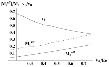
b)

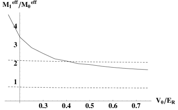
Figure 2: a) Group velocity and absolute value of effective masses as a function of the optical lattice depth $V_{0}$. b) Fullfillment of condition (53) as a function of $V_{0}$. The solid line represents $M^{\mbox{{\scriptsize eff}}}_{1}/M^{\mbox{{\scriptsize eff}}}_{0}$, the dashed lines are the upper and lower bound in the inequality (53). For $V_{0}>0.4E_{R}$ the condition is fullfilled.

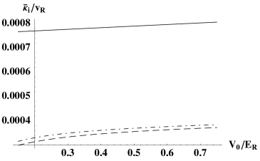
Figure 3: Interaction parameters as a function of lattice depth $V_{0}$ in units of the recoil velocity $v_{R}=\sqrt{2E_{R}/M}$. Solid line: $\bar{\kappa}_{0}$, dashed line: $\bar{\kappa}_{1}$, dot-dashed line: $\bar{\kappa}_{01}$.

a)

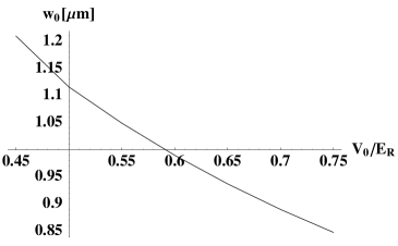
b)

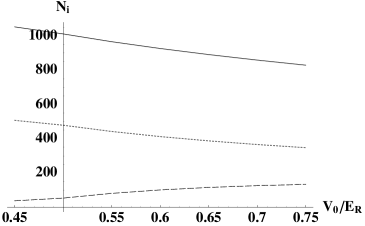
Figure 4: a) Width of the soliton wavepackets as a function of $V_{0}$. b) Total number of atoms $N$ (solid line) in the soliton, and number of atoms $N_{i}=A_{i}^{2}N/L$ in mode $i=0$ (dashed line) and $i=1$ (dotted line), respectively.