Statistics of excitons in quantum dots and the resulting microcavity emission spectra

Abstract

A theoretical investigation is presented of the statistics of excitons in quantum dots (QDs) of different sizes. A formalism is developed to build the exciton creation operator in a dot from the single exciton wavefunction and it is shown how this operator evolves from purely fermionic, in case of a small QD, to purely bosonic, in case of large QDs. Nonlinear optical emission spectra of semiconductor microcavities containing single QDs are found to exhibit a peculiar multiplet structure which reduces to Mollow triplet and Rabi doublet in fermionic and bosonic limits, respectively.

I Introduction

Semiconductor quantum dots (QDs) Bimberg et al. (1998) are a leading technology for the investigation of the quantum realm. They offer exciting possibilities for quantum computation and are important candidates for the next generation of light emitters. In most cases, the best control of the states of the confined carriers in QDs is obtained through coupling to light Ivchenko (2005). This light-matter interaction can be considerably enhanced by including the dot in a microcavity, with pillars Reithmaier et al. (2004), photonic crystals Yoshie et al. (2004) and microdisks Peter et al. (2005) being the currently favoured realizations. References [Reithmaier et al., 2004; Yoshie et al., 2004; Peter et al., 2005] describe the first reports, in each of these structures, of vacuum field Rabi splitting, whereby one excitation is transferred back and forth between the light and the matter fields. This contrasts with the weak coupling regime previously studied,Gérard et al. (1998); Solomon et al. (2000) where only quantitative perturbations of the dynamics occur, such as reductions in the lifetimes of the dot excitations (Purcell effect). In the case of strong coupling, however, the coherent exchange of energy merges the light and matter excitations into a new entity. This is commonly referred to as an exciton-polariton in semiconductor physics, Kavokin and Malpuech (2003) with an important example being the two-dimensional polaritons in planar microcavities, first observed by Weisbuch et al. Weisbuch et al. (1992) In cavity quantum electrodynamics (cQED), the equivalent concept is the dressed state of atoms by the quantised electromagnetic field.

In QDs, optical interband excitations create electron-hole pairs or excitons, confined by a three-dimensional potential which makes their energy spectrum discrete. If this potential is much stronger than the bulk exciton binding energy, and if the size of the dot is smaller than the corresponding exciton Bohr radius, the Coulomb interaction between electrons and holes can be considered as a perturbation. For the lowest exciton states, this is the fermionic limit where the Pauli exclusion principle dominates. In the opposite limit, if the confining potential is weak or the size of the dot is much greater than the exciton Bohr radius, the exciton is quantized as a whole particle. In this case, the bosonic nature of excitons is expected to prevail over fermionic nature of individual electrons and holes. An important question for the description of emission from QDs embedded into cavities in the strong coupling regime is whether the dot excitations coupled to light behave like fermions or like bosons. Here we address the question of which statistics (Bose-Einstein, Fermi-Dirac or a variation thereof) best describes excitons in QDs. This is a question which is very topical in view of the recent experimental achievements, and which has elicited substantial theoretical works in the past, in connection with the possibility of exciton Bose condensation.

In this paper we derive the exciton creation operator in a QD which allows the calculation of nonlinear optical spectra of QDs in microcavities. The model we develop takes into account the saturation of the transition due to Pauli exclusion alone and does not attempt to solve the complex manybody problem which arises when Coulomb interactions between excitons are included. Hence the model is most accurate in describing the departure from ideal bosonic behaviour in large dots rather than near the fermionic limit in small dots. We analyze the dot size effect on the statistics of excitons and demonstrate the transition from the fermionic to bosonic regime. To motivate this, we begin by summarizing how the coupling of light modes with fermionic and bosonic material excitations differ.

The Rabi doublet, with splitting amplitude $2\hbar g$ as shown on Fig. 1(a), is well accounted for theoretically by the coupling with strength $\hbar g$ of two quantized oscillators $a$ and $b$ both obeying Bose algebra,

$$[a,{a^{\dagger}}]=1,$$ (1)

and equivalently for  $b$. We shall describe this well known and elementary case in detail as it provides the foundation for most of what follows. Neglecting off-resonant terms like ${a^{\dagger}}{b^{\dagger}}$, the hamiltonian reads Carmichael (2002)

$$H=\hbar\omega({a^{\dagger}}a+{b^{\dagger}}b)+\hbar g(a{b^{\dagger}}+{a^{\dagger}}b)\,.$$ (2)

We assumed degenerate energies $\hbar\omega$ for the two oscillators, which will not affect our qualitative results, while simplifying considerably the analytical expressions. One oscillator, say $a$, describes the light field while the other, $b$, describes a bosonic matter field. The analysis of (2) can be made directly in the bare state basis $\left|i,j\right\rangle$ with $i$ excitations in the matter field and $j$ in the photonic field, $i$, $j\in\mathbf{N}$. The value of this approach is that the excitation, loss and dephasing processes generally pertain to the bare particles. For instance matter excitations are usually created by an external source (pumping) and light excitations can be lost by transmission through the cavity mirror. This physics is best expressed in the bare states basis.

Figure 1: (Color online) Energy diagrams of the two limiting cases of dressed bosons (left) and fermions (right). In the first case the $n$th manifold has constant energy splitting of $2\hbar g$ between all states and couples to the $(n-1)$th manifold by removal of a quantum of excitation with energy $\hbar\omega\pm\hbar g$ which leads to the Rabi doublet, Fig. (a), with splitting $2\hbar g$. In the second case, each manifold is two-fold with a splitting which increases like a square root. All four transitions are allowed, leading to the Mollow triplet, Fig. (b), for high values of $n$ when the two middle transitions are close in energy. The distance from the central peak goes like $2\hbar g\sqrt{n}$ and the ratio of peaks is $1:2$. The two lowest manifolds (in blue) are the same in both cases, making vacuum field Rabi splitting insensitive to the statistics.

On the other hand (2) assumes a straightforward expression in the basis of so-called dressed states which diagonalises the Hamiltonian to read:

$$H=(\hbar\omega-\hbar g){p^{\dagger}}p+(\hbar\omega+\hbar g){q^{\dagger}}q$$ (3)

where ${p^{\dagger}}$ and ${q^{\dagger}}$ create a coherent superposition of bare states, respectively in and out of phase:

$$p=(a+b)/\sqrt{2},\qquad q=(a-b)/\sqrt{2}\,.$$ (4)

For clarity we shall note $|\kern-1.87772pt|i,j\rangle\kern-2.84544pt\rangle$ the dressed states, i.e., the eigenstates of (3) with $i$ dressed particles of energy $\hbar\omega-\hbar g$ and $j$ of energy $\hbar\omega+\hbar g$. The manifold of states with $n$ excitations thus reads, in the dressed states basis:

$$\mathcal{H}_{n}=\{|\kern-1.87772pt|i,j\rangle\kern-2.84544pt\rangle~{};~{}i,j\in\mathbf{N}~{}\mathrm{with}~{}i+j=n\}$$ (5)

Its energy diagram appears on the left of Fig. 1 for manifolds with zero (vacuum), one, two and seven excitations. When an excitation escapes the system while in manifold $\mathcal{H}_{n}$, a transition is made to the neighbouring manifold $\mathcal{H}_{n-1}$ and the energy difference is carried away, either by the leaking out of a cavity photon, or through exciton emission into a radiative mode other than that of the cavity, or a non-radiative process. The detailed analysis of such processes requires a dynamical study, but as the cavity mode radiation spectra can be computed with the knowledge of only the energy level diagrams, we shall keep our analysis to this level for the present work. The important feature of this dissipation is that, though such processes involve $a$ or $b$ (rather than $p$ or $q$), they nevertheless still result in removing one excitation out of one of the oscillators. Hence only transitions from $|\kern-1.87772pt|i,j\rangle\kern-2.84544pt\rangle$ to $|\kern-1.87772pt|i-1,j\rangle\kern-2.84544pt\rangle$ or $|\kern-1.87772pt|i,j-1\rangle\kern-2.84544pt\rangle$ are allowed, bringing away, respectively, $\hbar\omega+\hbar g$ and $\hbar\omega-\hbar g$ of energy, accounting for the so-called Rabi doublet (provided the initial $i$ and $j$ are nonzero in which case only one transition is allowed). From the algebraic point of view, this of course follows straightforwardly from (4) and orthogonality of the basis states. Physically it comes from the fact that, as in the classical case, the coupled system acts as two independent oscillators vibrating with frequencies $\omega\pm g$. In the case of vacuum field Rabi splitting, a single excitation is shared between the two fields, and so the manifold $\mathcal{H}_{1}$ is connected to the single line of the vacuum manifold. In this case there is obviously no possibility beyond a doublet.

Different physics occurs when the excitations of the material are described by fermionic rather than bosonic statistics. In the case of cavity QED the material is usually a beam of atoms passing through the cavity, and a single excitation is the independent responses of the atoms to the light field excitation. The simplest situation is that of a dilute atomic beam where a single atom (driven at resonance so that it appears as a two-levels system) is coupled to a Fock state of light with a large number of photons. This case is described theoretically by the Jaynes-Cummings model Jaynes and Cummings (1963), in which $a$ (the radiation field) remains a Bose operator but $b$ becomes a fermionic operator which describes two-levels systems, ${b^{\dagger}}\rightarrow\sigma_{+}$ with :

$$\sigma_{+}=\begin{pmatrix}0&1\\ 0&0\end{pmatrix}.$$ (6)

Then the atom must be in either the ground or the excited state, allowing for the manifolds

$$\mathcal{H}_{n}=\{\left|0,n\right\rangle,\left|1,n-1\right\rangle\}$$ (7)

provided that $n\geq 1$. The associated energy diagrams appear on the right of Fig. 1, with two states in each manifold (in our conventions $\left|0,n\right\rangle$ refers to the bare states with atom in ground state and $n$ photons, while $\left|1,n-1\right\rangle$ has atom in excited state and $n-1$ photons). For the resonant condition, where the two-levels transition matches the cavity photon energy, the dressed states for this manifold are split by an energy $\sqrt{n}\hbar g$. In the general case, all four transitions between the states in manifolds $\mathcal{H}_{n}$ and $\mathcal{H}_{n-1}$ are possible, which results in a quadruplet. It is hard to resolve this quadruplet, but it has been done in Fourier transform of time resolved experiments Brune et al. (1996). It is simpler to consider photoluminescence directly under continuous excitation at high intensity (where the fluctuations of particles number have little effect). In this case, with $n\gg 1$, the two intermediate energies are almost degenerate and a triplet is obtained with its central peak being about twice as high as the two satellites. This is the Mollow triplet of resonance fluorescence Mollow (1969).

Thus we are faced with two limiting cases, one is a pure bosonic limit with equally spaced dressed states resulting in the linear Rabi doublet, the other the pure fermionic limit with pairs of dressed states of increasing splitting within a manifold but decreasing energy difference between two successive manifolds, giving rise to the Mollow triplet. In many of the strong coupling experiments conducted so far, and in all the reports concerning semiconductor QDs, only one single excitation is exchanged coherently, so that the states are dressed by the vacuum of the electromagnetic field, resulting in the Rabi doublet. However, at this level of excitation, there is complete agreement between the bosonic and fermionic models, with both providing a good description of the experimental observations. The prospect of stronger pumping, with more than one excitation shared between the two fields, makes it important to understand whether a realistic semiconductor QD will correspond to the bosonic or fermionic case, or something intermediate between the two.

We review and discuss some of the more significant achievements in this field in section II. In section III we lay down a general formalism for building the exciton creation operator. In section IV we study two limiting cases which resemble Bose and Fermi statistics. We show how in the general case the luminescence behaviour interpolates between these two limits which we have already discussed, and calculate the second order coherence of the emitted light. In section V we draw the experimental consequences of the various statistics and discuss how the spectra obtained allow a qualitative understanding of how excitations distribute themselves in the excitonic field. In the final section we conclude and discuss briefly ongoing work to refine the modelling of the excitonic wavefunction.

II Excitons as quasi-particles

The generic optical excitation in an intrinsic semiconductor is the electron-hole pair. In bulk, the two oppositely charged particles can be strongly correlated by the Coulomb interaction and bound as hydrogenic states (Wannier-Mott exciton). Although finding binding energies and wavefunctions for the single exciton case is a difficult problem in various geometries,D’Andrea and Sole (1990); Que (1992); He et al. (2005) as far as the vacuum coupling limit is concerned, the exciton field operator which links the two manifolds $\mathcal{H}_{1}$ and vacuum always assumes the simple form $\sigma_{+}$ regardless of the details of the exciton. As a particle constituted of two fermions, the exciton is commonly regarded as a boson, from consideration of the angular momentum addition rules and the spin-statistics theorem. For a single particle, this is an exact statement, albeit a trivial one. It is however generally agreed to hold at small densities Keldysh and Kozlov (1968). In this case the Rabi doublet is obtained, as observed experimentally Reithmaier et al. (2004); Yoshie et al. (2004); Peter et al. (2005).

At higher excitation power, the problem assumes considerable complexity as well as fundamental importance for physical applications. Already at the next higher excitation—with one more electron, hole or electron-hole pair added to the first exciton—the situation offers rich and various phenomena both in weak Besombes et al. (2002); Patton et al. (2003) and strong Ivanov et al. (1998) coupling, owing to the underlying complexity of the excitonic states. In this work we shall be concerned with resonant optical pumping, so that excitations are created in pairs and the system always remains electrically neutral. We shall describe as an exciton any state of an electron-hole pair, whether it is an atom-like 1$s$ state or has both particles independently quantised, Que (1992) and in a more general sense we shall also use the term for any combination of particles which takes part in the excitonic phase. Indeed the excitonic phase with more than one pair requires at the most accurate level a description in terms of an excitonic complex, e.g., in term of biexcitons/bipolaritons for strong coupling of two electrons and two holes with light Ivanov et al. (1998). This comes from the Coulomb interaction which links all charge carriers together and, in a most fundamental way, also from the antisymmetry of the wavefunction which demands a sign change whenever two identical fermions (electrons or holes) are swapped in the system. However in some configurations, especially in planar cavities, a widely accepted hypothesis of bosonic behavior of excitons and the derived polaritons has been investigated for effects such as the exciton boser Ĭmamoḡlu et al. (1996), polariton amplifier Savvidis et al. (2000); Ciuti et al. (2000); Rubo et al. (2003) and polariton lasers Deng et al. (2002); Laussy et al. (2004). The internal structure of the exciton which gives rise to both deviations from the Bose-statistics and interactions of the electron-hole pairs is then expressed as an effective repulsive force in a bosonised Hamiltonian (due to Coulomb interaction and Pauli effect in the form of phase-space filling or exchange interaction Ĭmamoḡlu (1998); Ciuti et al. (1998)).

This bosonic approach for excitons met early opposition in favour of an analysis in the electron-hole basis Kira et al. (1997); de Leon and Laikhtman (2001, 2003). Combescot and co-workers investigated the possibility of bosonisation of excitons Combescot and Tanguy (2001); Combescot and Betbeder-Matibet (2002a, b); Combescot and Betbeder-Matibet (2004) and concluded against it. They point out its internal inconsistency, as the same interaction binds the underlying fermions, and therefore defines the exciton, while also being responsible for exciton-exciton scattering; this is inconsistent with the indistinguishability of the particles. These authors introduce the “proteon” as the paradigm for Bose-like composite particle and propose a formalism (“commutation technics”) which essentially relies on evaluating quantum correlators in the fermion basis with operators linked through the single exciton wave-function. The importance of Fermi statistics of the underlying constituents has also been pointed out by Rombouts and co-workers in connection to atomic and excitonic condensates Rombouts et al. (2002, 2005). In both cases the composite “boson” creation operator reads

$${B^{\dagger}}=\sum_{\mathbf{k}}\phi_{\mathbf{k}}{\sigma_{\mathbf{k}}^{\dagger}}{\varsigma_{-\mathbf{k}}^{\dagger}}$$ (8)

in term of $\sigma_{\mathbf{k}}$, $\varsigma_{\mathbf{k}}$ the fermion operators

$$\{\sigma_{\mathbf{k}},{\sigma_{\mathbf{k}^{\prime}}^{\dagger}}\}=\delta_{\mathbf{k},\mathbf{k}^{\prime}},\qquad\{\sigma_{\mathbf{k}},\sigma_{\mathbf{k}^{\prime}}\}=0$$ (9)

(same for $\varsigma_{\mathbf{k}}$), respectively for an electron and hole (or proton in the atomic case Rombouts et al. (2005)) of momentum $\mathbf{k}$. This operator creates excitons with the center-of-mass momentum $\mathbf{K}=\mathbf{0}$ in a system with translational invariance. It was appreciated long agoKeldysh and Kozlov (1968) that the operators ${B^{\dagger}}$ and $B$ are no-longer exact bosonic operators, but instead satisfy,

$$[B,{B^{\dagger}}]=1-D,$$ (10)

where $D$ is a nonzero operator, though with small matrix elements at low exciton densities.

Our approach is based on a definition similar to Eq. (8) for the exciton operator. Instead of analysing the deviations in the commutation relationship (10) we derive the matrix elements of the operator ${B^{\dagger}}$. The direct analysis of these matrix elements allows us to trace departures from Bose-statistics and to investigate the transitions between bosonic and fermionic behaviours of excitons in QDs. We shall compare our results with those of Refs. [Combescot and Tanguy, 2001; Combescot and Betbeder-Matibet, 2002a, b; Combescot and Betbeder-Matibet, 2004; Rombouts et al., 2002, 2005]. For convenience, we will refer to these two sets of publications through the names of their first authors, keeping in mind that they are co-authored papers, as listed in the references.

III Formalism

We consider a QD, which localises the excitation in real space. Thus our main departure from Combescot and Rombouts is that our exciton creation operator, ${X^{\dagger}}$, is expressed in real space and without the zero center-of-mass momentum restriction,

$${X^{\dagger}}=\sum_{n_{e},n_{h}}C_{n_{e},n_{h}}{\sigma_{n_{e}}^{\dagger}}{\varsigma_{n_{h}}^{\dagger}}$$ (11)

where $\sigma_{n_{e}}$ and $\varsigma_{n_{h}}$ are fermion creation operators, cf. (9), for an electron and a hole in state $\left|\varphi^{e}_{n_{e}}\right\rangle$ and $\left|\varphi^{h}_{n_{h}}\right\rangle$, respectively:

$${\sigma_{n_{e}}^{\dagger}}\left|0\right\rangle=\left|\varphi^{e}_{n_{e}}\right\rangle,\quad{\varsigma_{n_{h}}^{\dagger}}\left|0\right\rangle=\left|\varphi^{h}_{n_{h}}\right\rangle,$$ (12)

with $\left|0\right\rangle$ denoting both the electron and hole vacuum fields. We carry out the analysis in real space with the set of basis wavefunctions

$$\varphi^{e}_{n_{e}}(\mathbf{r}_{e})=\langle\mathbf{r}_{e}|\varphi^{e}_{n_{e}}\rangle\quad\mathrm{and}\quad\varphi^{h}_{n_{h}}(\mathbf{r}_{h})=\langle\mathbf{r}_{h}|\varphi^{h}_{n_{h}}\rangle$$ (13)

with $\mathbf{r}_{e}$ and $\mathbf{r}_{h}$ the positions of the electron and hole, respectively. Subscripts $n_{e}$ and $n_{h}$ are multi-indices enumerating all quantum numbers of electrons and holes. The specifics of the three-dimensional confinement manifests itself in the discrete character of $n_{e}$ and $n_{h}$ components.

We restrict our considerations to the direct band semiconductor with non-degenerate valence band. Such a situation can be experimentally achieved in QDs formed in conventional III-V or II-VI semiconductors, where the light-hole levels lie far, in energy, heavy-hole ones due to the effects of strain and size quantization along the growth axisIvchenko (2005). Therefore, only electron-heavy hole excitons need to be considered. Moreover, we will neglect the spin degree of freedom of the electron-hole pair and assume all carriers to be spin polarized. This can be realized by pumping the system with light of definite circular polarization, as spin-lattice relaxation is known to be very inefficient in QDs.

The (single) exciton wavefunction $\left|\varphi\right\rangle$ results from the application of ${X^{\dagger}}$ on the vacuum. In real space coordinates:

$$\langle\mathbf{r}_{e},\mathbf{r}_{h}|\varphi\rangle=\varphi(\mathbf{r}_{e},\mathbf{r}_{h})=\sum_{n_{e},n_{h}}C_{n_{e},n_{h}}\varphi^{e}_{n_{e}}(\mathbf{r}_{e})\varphi^{h}_{n_{h}}(\mathbf{r}_{h}).$$ (14)

At this stage we do not specify the wavefunction (that is, the coefficients $C_{n_{e},n_{h}}$), which depends on various factors such as the dot geometry, electron and hole effective masses and dielectric constant. Rather, we consider the $n$ excitons state which results from successive excitation of the system through ${X^{\dagger}}$:

$$\left|\Psi_{n}\right\rangle=({X^{\dagger}})^{n}\left|0\right\rangle,$$ (15)

We later discuss in more details what approximations are being made here. For now we proceed by normalising this wavefunction

$$\left|n\right\rangle={1\over\mathcal{N}_{n}}\left|\Psi_{n}\right\rangle$$ (16)

where, by definition of the normalization constant

$$\mathcal{N}_{n}=\sqrt{\langle\Psi_{n}|\Psi_{n}\rangle}.$$ (17)

The creation operator ${X^{\dagger}}$ can now be obtained explicitly. We call $\alpha_{n}$ the non-zero matrix element which lies below the diagonal in the excitons representation:

$$\alpha_{n}=\langle n|{X^{\dagger}}|n-1\rangle\,,$$ (18)

which, by comparing Eqs. (15–18) turns out to be

$$\alpha_{n}=\frac{\mathcal{N}_{n}}{\mathcal{N}_{n-1}}\,.$$ (19)

We now undertake to link $\alpha_{n}$ with the coefficients $C_{n_{e},n_{h}}$, which assume a specific form only when the system itself has been characterised. The general relationship is more easily obtained in the real space than with the operator representation (11). Indeed the non-normalized $n$-excitons wavefunction assumes the simple form of a Slater determinant

$$\Psi_{n}(\mathbf{r}_{e_{1}},\ldots,\mathbf{r}_{e_{n}},\mathbf{r}_{h_{1}},\ldots,\mathbf{r}_{h_{n}})=\det_{1\leq i,j\leq n}{[\varphi(\mathbf{r}_{e_{i}},\mathbf{r}_{h_{j}})]},$$ (20)

explicitly ensuring the antisymmetry of $\Psi_{n}$ upon exchange of two identical fermions (holes and electrons), as results from the anticommutation rule (9) in the $n$th power of operator ${X^{\dagger}}$, cf. (11).

The determinant can be computed explicitly, by expansion of its minors which results in the recurrent relation

$$\mathcal{N}_{n}^{2}={1\over n}\sum_{m=1}^{n}(-1)^{m+1}\beta_{m}\mathcal{N}_{n-m}^{2}\prod_{j=0}^{m-1}(n-j)^{2},$$ (21)

with $\mathcal{N}_{0}=1$ and $\beta_{m}$ the irreducible $m$-excitons overlap integrals, $1\leq m\leq n$:

$$\beta_{m}=\int\left(\prod_{i=1}^{m-1}\varphi^{*}(\mathbf{r}_{e_{i}},\mathbf{r}_{h_{i}})\varphi(\mathbf{r}_{e_{i}},\mathbf{r}_{h_{i+1}})\right)\varphi^{*}(\mathbf{r}_{e_{m}},\mathbf{r}_{h_{m}})\varphi(\mathbf{r}_{e_{m}},\mathbf{r}_{h_{1}})\,d\mathbf{r}_{e_{1}}\dots d\mathbf{r}_{e_{m}}d\mathbf{r}_{h_{1}}\dots d\mathbf{r}_{h_{m}}$$ (22)

The determinant can also be solved by direct combinatorial evaluation, counting all combinations which can be factored out as products of $\beta_{m}$. The result expressed in this way reads:

$$\mathcal{N}_{n}^{2}=\sum_{\eta=1}^{p(n)}C_{n}(\eta)\prod_{m=1}^{N}\beta_{m}^{\nu_{\eta}(m)}$$ (23)

where $p(n)$ is the partition function of $n$ (number of ways to write $n$ as a sum of positive integers, i.e., as an integer partition of $n$) and $\nu_{\eta}(i)$ is the number of times that $i\in\mathbf{N}$ appears in the $\eta^{\mathrm{th}}$ partition of $n$. The coefficients $C_{n}$ read:

$$C_{n}(\eta)\equiv n!(-1)^{n+\sum_{m=1}^{n}\nu_{\eta}(m)}\prod_{\{n_{i}\}}{n-\sum_{j=1}^{i-1}n_{j}\choose n_{i}}{(n_{i}-1)!\over\nu_{\eta}(i)!}$$

where the product is taken over the integers $n_{i}$ which enter in the $\eta^{\mathrm{th}}$ partition of $n$, i.e., $n=\sum_{i}n_{i}$.

The procedure to calculate the matrix elements of the creation operator is as follows: One starts from the envelope function $\varphi(\mathbf{r}_{e},\mathbf{r}_{h})$ for a single exciton. Then one calculates all overlap integrals $\beta_{m}$ as given by (22), for $1\leq m\leq n$ where $n$ is the highest manifold to be accessed. Then the norms can be computed, the more practical way being recursively with (21). Finally the matrix elements $\alpha_{n}$ are obtained as the successive norms ratio, cf. (18). Once $\alpha_{n}$ are known the emission spectra can be calculated with ease. We note here that the numerical computation of the $\beta_{m}$ and $\alpha_{n}$ values needs to be carried out with great care. The cancellation of the large numbers of terms involved in Eq. (21) requires a very high-precision evaluation of $\beta_{m}$.

Although derived from the formulation in real space (20), the recurrent relation (21), or its analytical solution (23), is a property of fermion pairs, so it applies to the fermionic operators in (8) as well. The core of the mathematical results contained in these two expressions has in fact been obtained by Combescot Combescot and Tanguy (2001) through direct evaluation with the operator algebra involved in ${B^{\dagger}}$. The only difference with her approach and ours is that her corresponding quantity $\beta_{m}$ (which she notes $\sigma_{m}$) appears as a series in the (reciprocal space) wavefunction

$$\sigma_{m}=\sum_{\mathbf{k}}|\phi_{\mathbf{k}}|^{2m}$$ (24)

as opposed to the overlap integral (22).

With such a simple expression as (24), Combescot et al. have been able to obtain approximate analytical forms for 1$s$ states of excitons in both 3D and 2D. The sum over reciprocal space is approximated as an integral in the continuum limit, and since $\phi_{\mathbf{k}}$ depends on $k=|\mathbf{k}|$ only, this becomes $\sum_{\mathbf{k}}|\phi_{\mathbf{k}}|^{2m}\rightarrow\int\mathcal{V}_{k}|\phi_{k}|^{2m}dk$ with $\mathcal{V}_{k}=4\pi k^{2}$ or $2\pi k$, respectively, yielding Combescot and Tanguy (2001)

$$\sigma_{m} =z^{m-1}16{(8m-5)!!\over(8m-2)!!} \mathrm{in~{}3D},$$ (25)

$$\sigma_{m} ={2y^{m-1}\over 3m-1} \mathrm{in~{}2D},$$ (26)

with $z$ and $y$ dimensionless parameters involving the ratio of Bohr radius $a_{\mathrm{B}}$ to the size of the system. In Ref. [Combescot and Tanguy, 2001], this continuous approximation is used even when the system size becomes so small that the quantization becomes noticeable, as a result of which a negative norm is obtained even for a well defined wavefunction. However, the authors interpret incorrectly this negative norm as the result of an unphysical exciton wavefunction and thus the breakdown of the bosonic picture. To demonstrate this, we have computed numerically the values of $\sigma_{m}$ by direct summation of Eq. (24) and used them to evaluate normalization constants $\mathcal{N}_{n}$. Some results of the computation are shown in Fig. 2. The inset shows the dependence of $\mathcal{N}_{1}\equiv\sigma_{1}$ vs. the ratio of crystal size $L$ to 3D exciton Bohr radius $a_{\mathrm{B}}$. The continuous approximation Eq. (25) gives $\sigma_{1}=1$, shown by the dashed line in the inset. The solid line displays the value of $\sigma_{1}$ computed exactly with (24): it approaches $1$ when $L/a_{\mathrm{B}}\to\infty$ but departs strongly from 1 as the size of the system reduces, since the real wavefunction changes as the system shrinks about it. At the very least this needs to be taken into account by correcting the normalization constant of $\phi_{\mathbf{k}}$, as otherwise unphysical result may arise. The main part of the figure shows the two-excitons normalization $\mathcal{N}_{2}$ calculated by both methods. We find that for all $L/a_{\rm B}$, the exact $\mathcal{N}_{2}$ never becomes negative in clear constrast with the behavior obtained with the approximated value (25). Hence it is not possible to use the appearance of a negative norm as a criterion for bosonic breakdown.

Figure 2: Normalization constant $\mathcal{N}_{2}$ vs. ratio of crystal size $L$ to 3D exciton Bohr radius $a_{\mathrm{B}}$. Dashed line shows the result using the approximated expression (25) for $\sigma_{m}$ and solid line using the exact evaluation of the sum on the mesh in reciprocal space. The negative value of the norm used as a criterion for boson wavefunction breakdown in Ref. [Combescot and Tanguy, 2001] is an artifact of this approximation. With the genuine wavefunction, our procedure yields a non-arbitrary way to consider how the wavefunction vanishing norm affects the bosonic character of the excitation. Inset displays $\mathcal{N}_{1}$ vs. $L/a_{\mathrm{B}}$ computed on mesh (solid) and according to Eq. (25) (dashes).

IV Limiting cases

We shall not attempt in this paper to go through the lenghty and complicated task of the numerical calculation of the exciton creation operator matrix elements for a realistic QD. Rather, we consider here a model wavefunction which can be integrated analytically and illustrates some expected typical behaviours. Before this, we comment briefly on the limiting cases of Bose-Einstein and Fermi-Dirac statistics and how they can be recovered in the general setting of this section.

This will be made most clear through consideration of the explicit case of two excitons ($n=2$). Then the wavefunction reads

$$\Psi_{2}(\mathbf{r}_{e_{1}},\mathbf{r}_{e_{2}},\mathbf{r}_{h_{1}},\mathbf{r}_{h_{2}})=\varphi(\mathbf{r}_{e_{1}},\mathbf{r}_{h_{1}})\varphi(\mathbf{r}_{e_{2}},\mathbf{r}_{h_{2}})\\ -\varphi(\mathbf{r}_{e_{1}},\mathbf{r}_{h_{2}})\varphi(\mathbf{r}_{e_{2}},\mathbf{r}_{h_{1}})$$ (27)

with its normalization constant (17) readily obtained as

$$\mathcal{N}_{2}^{2}=\int|\Psi_{2}(\mathbf{r}_{e_{1}},\mathbf{r}_{e_{2}},\mathbf{r}_{h_{1}},\mathbf{r}_{h_{2}})|^{2}d\mathbf{r}_{e_{1}}\ldots d\mathbf{r}_{h_{2}}=2-2\beta_{2}$$ (28)

where $\beta_{2}$, the two-excitons overlap integral, reads explicitly

$$\beta_{2}=\int\varphi(\mathbf{r}_{e_{1}},\mathbf{r}_{h_{1}})\varphi(\mathbf{r}_{e_{2}},\mathbf{r}_{h_{2}})\\ \varphi(\mathbf{r}_{e_{1}},\mathbf{r}_{h_{2}})\varphi(\mathbf{r}_{e_{2}},\mathbf{r}_{h_{1}})d\mathbf{r}_{e_{1}}\ldots d\mathbf{r}_{h_{2}}.$$ (29)

This integral is the signature of the composite nature of the exciton. The minus sign in (28) results from the Pauli principle: two fermions (electrons and holes) cannot occupy the same state. Assuming $\varphi(\mathbf{r}_{e},\mathbf{r}_{h})$ is normalised, $\mathcal{N}_{1}=1$, so according to (19),

$$\alpha_{2}=\sqrt{2-2\beta_{2}}.$$ (30)

Since $0\leq\beta_{2}\leq 1$ this is smaller than or equal to $\sqrt{2}$, the corresponding matrix element of a true boson creation operator. This result has a transparent physical meaning: since two identical fermions from two excitons cannot be in the same quantum state, it is “harder” to create two real excitons, where underlying structure is probed, than two ideal bosons. We note that if $L$ is the QD lateral dimension, $\beta_{2}\sim(a_{\mathrm{B}}/L)^{2}\ll 1$ when $L\gg a_{\mathrm{B}}$. Thus in large QDs the overlap of excitonic wavefunctions is small, so $\alpha_{2}\approx\sqrt{2}$ and the bosonic limit is recovered. On the other hand, in a small QD, where Coulomb interaction is unimportant compared to the dot potential confining the carriers, the electron and hole can be regarded as quantized separately:

$$\varphi(\mathbf{r}_{e},\mathbf{r}_{h})=\varphi^{e}(\mathbf{r}_{e})\varphi^{h}(\mathbf{r}_{h})$$ (31)

In this case all $\beta_{m}=1$ and subsequently all $\alpha_{m}=0$ at the exception of $\alpha_{1}=1$. This is the fermionic limit where ${X^{\dagger}}$ maps to the Pauli matrix $\sigma_{+}$, cf. (6).

We now turn to the general case of arbitrary sized QDs, interpolating between the (small) fermionic and (large) bosonic limits. We assume a Gaussian form for the wavefunction which allows to evaluate analytically all the required quantities. As numerical accuracy is not the chief goal of this work we further assume in-plane coordinates $x$ and $y$ to be uncorrelated to ease the computations. The wavefunction reads:

$$\varphi(\mathbf{r}_{e},\mathbf{r}_{h})=\mathcal{C}\exp(-\gamma_{e}\mathbf{r}_{e}^{2}-\gamma_{h}\mathbf{r}_{h}^{2}-\gamma_{eh}\mathbf{r}_{e}\cdot\mathbf{r}_{h})$$ (32)

properly normalized with

$$\mathcal{C}={\sqrt{4\gamma_{e}\gamma_{h}-\gamma_{eh}^{2}}\over\pi}$$ (33)

provided that $\gamma_{eh}\in[-2\sqrt{\gamma_{e}\gamma_{h}},0]$ with $\gamma_{e}$, $\gamma_{h}\geq 0$. The $\gamma$ parameters allow to interpolate between the large and small dot limits within the same wavefunction. To connect these parameters $\gamma_{e}$, $\gamma_{h}$ and $\gamma_{eh}$ to physical quantities, (32) is regarded as a trial wavefunction which is to minimize the hamiltonian $H_{\mathrm{QD}}$ confining the electron and hole in a quadratic potential where they interact through Coulomb interactionQue (1992):

$$H_{\mathrm{QD}}=\sum_{i=e,h}\left({\mathbf{p}_{i}^{2}\over 2m_{i}}+{1\over 2}m_{i}\omega^{2}\mathbf{r}_{i}^{2}\right)-{e^{2}\over\epsilon|\mathbf{r}_{e}-\mathbf{r}_{h}|}$$ (34)

Here $\mathbf{p}_{i}$ the momentum operator for the electron and hole, $i=\mathrm{e}$, $\mathrm{h}$, respectively, $m_{e}$, $m_{h}$ the electron and hole masses, $\omega$ the frequency which characterises the strength of the confining potential, $e$ the charge of the electron and $\epsilon$ the background dielectric constant screening the Coulomb interaction. This hamiltonian defines the two length scales of our problem, the 2D Bohr radius $a_{\mathrm{B}}$ and the dot size $L$:

$$a_{\mathrm{B}} = {\epsilon\hbar^{2}\over 2\mu e^{2}}$$ (35a)

$$L = \sqrt{\hbar\over\mu\omega}$$ (35b)

where $\mu=m_{e}m_{h}/(m_{e}+m_{h})$ is the reduced mass of the electron-hole pair. To simplify the following discussion we assume that $m_{e}=m_{h}$, resulting in $\gamma_{e}=\gamma_{h}=\gamma$. The trial wavefunction (32) separates as $\varphi(\mathbf{r}_{e},\mathbf{r}_{h})=\mathcal{C}\Phi(\mathbf{R})\phi(\mathbf{r})$ where $\mathbf{r}=\mathbf{r}_{e}-\mathbf{r}_{h}$ is the radius-vector of relative motion and $\mathbf{R}=(\mathbf{r}_{e}+\mathbf{r}_{h})/2$ is the center-of-mass position:

$$\Phi(\mathbf{R}) = {\sqrt{2(2\gamma+\gamma_{eh})}\over\sqrt{\pi}}\exp{\left(-\mathbf{R}^{2}[2\gamma+\gamma_{eh}]\right)}$$ (36a)

$$\phi(\mathbf{r}) = {\sqrt{2\gamma-\gamma_{eh}}\over\sqrt{2\pi}}\exp{\left(-\mathbf{r}^{2}\left[{2\gamma-\gamma_{eh}\over 4}\right]\right)}$$ (36b)

Eq. (36a) is an eigenstate of the center-of-mass energy operator and equating its parameters with those of the exact solution yields the relationship $2\gamma+\gamma_{eh}={2/L^{2}}$. This constrain allows to minimise (36b) with respect to a single parameter, $a=-\gamma_{eh}/2+1/(2L^{2})$, which eventually amounts to minimise ${4a_{\mathrm{B}}/a^{2}}+{a_{\mathrm{B}}a^{2}/L^{4}}-{2\sqrt{\pi}/a}$. Doing so we have obtained the ratio $-\gamma_{eh}/\gamma$ as a function of $L/a_{\mathrm{B}}$ displayed on Fig. 3. The transition from bosonic to fermionic regime is seen to occur sharply when the dot size becomes commensurable with the Bohr radius.

Figure 3: Ratio of parameters $-\gamma_{eh}$ and $\gamma$ (with $\gamma=\gamma_{e}=\gamma_{h}$) as a function of $L/a_{\mathrm{B}}$. For large dots where $L\gg a_{\mathrm{B}}$, $-\gamma_{eh}/\gamma\approx 2$ which corresponds to the bosonic limit where the electron and hole are strongly correlated. For shallow dots where $L\ll a_{\mathrm{B}}$, $-\gamma_{eh}/\gamma\approx 0$ with electron and hole quantized separately. The transition is shown as the result of a variational procedure, with an abrupt transition when the dot size becomes comparable to the Bohr Radius.

For large dots, i.e., for large values of $L/a_{\mathrm{B}}$, the ratio is well approximated by the expression

$$-\gamma_{eh}/\gamma=2-(a_{\mathrm{B}}/L)^{2}$$ (37)

so that in the limit $a_{\mathrm{B}}/L\rightarrow 0$, Eq. (32) reads $\varphi(\mathbf{r}_{e},\mathbf{r}_{h})\propto{\exp(-(\sqrt{\gamma_{e}}\mathbf{r}_{e}-\sqrt{\gamma_{h}}\mathbf{r}_{h})^{2})}$ with vanishing normalization constant. This mimics a free exciton in an infinite quantum well. It corresponds to the bosonic case. On the other hand, if $L$ is small compared to the Bohr radius, with $\gamma_{eh}\rightarrow 0$, the limit (31) is recovered with $\varphi\propto\exp(-\gamma_{e}\mathbf{r}_{e}^{2})\exp(-\gamma_{h}\mathbf{r}_{h}^{2})$. This corresponds to the fermionic case.

One can readily check that (32) gives, in the case $\gamma_{eh}\rightarrow-2\sqrt{\gamma_{e}\gamma_{h}}$, an exciton binding energy which is smaller by only $20\%$ than that calculated with a hydrogenic wavefunction, which shows that the Gaussian approximation should be tolerable for qualitative and semi-quantitative results. Moreover, its form corresponds to the general shape of a trial wavefunction for an exciton in an arbitrary QD, Semina et al. (2005) with the only difference that we take the Gaussian expression instead of a Bohr exponential for the wavefunction of the relative motion of the electron and hole. This compromise to numerical accuracy allows on the other hand to obtain analytical expressions for all the key parameters, starting with the overlap integrals (22) which take a simple form in terms of multivariate Gaussians:

$$\beta_{m}=\mathcal{C}^{2m}\int\exp(-{\bf x}^{T}A{\bf x})\,d{\bf x}\int\exp(-{\bf y}^{T}A{\bf y})\,d{\bf y}$$ (38)

where

$$\mathbf{x}^{T}=(x_{e_{1}},x_{e_{2}},\ldots,x_{e_{m}},x_{h_{1}},x_{h_{2}},\ldots,x_{h_{m}})$$ (39a)

$$\mathbf{y}^{T}=(y_{e_{1}},y_{e_{2}},\ldots,y_{e_{m}},y_{h_{1}},y_{h_{2}},\ldots,y_{h_{m}})$$ (39b)

are the $2m$ dimensional vectors which encapsulate all the degrees of freedom of the $m$ excitons-complex, and $A$ is a positive definite symmetric matrix which equates (22) and (38), i.e., which satisfies

$${\bf x}^{T}A{\bf x}=2\gamma_{e}\sum_{i=1}^{m}x_{i}^{2}+2\gamma_{h}\sum_{i=m+1}^{2m}x_{i}^{2}+\gamma_{eh}x_{m}x_{m+1}\\ +\gamma_{eh}\sum_{i=1}^{m}x_{i}x_{m+i}+\gamma_{eh}\sum_{i=1}^{m-1}x_{i}x_{m+i+1}$$ (40)

and likewise for $\mathbf{y}$ (to simplify notation we have not written an index $m$ on $\mathbf{x}$, $\mathbf{y}$ and $A$, but these naturally scale with $\beta_{m}$). The identity for $2m$-fold Gaussian integrals

$$\int\exp(-{\bf x}^{T}A{\bf x})\,d{\bf x}={\pi^{m}\over\sqrt{\det{A}}}$$ (41)

allows us to obtain an analytical expression for $\beta_{m}$, although a cumbersome one. The determinant of the matrix $A$ reads

$$\det{A}={\gamma_{eh}}^{2m}\sum_{k=0}^{m}\sum_{l=0}^{m-k}(-1)^{\lfloor m/2\rfloor+k}\mathcal{A}_{m}(k,l)\left({\gamma_{e}\gamma_{h}\over{\gamma_{eh}}^{2}}\right)^{k}.$$ (42)

Here we introduced a quantity

$$\mathcal{A}_{m}(k,l)=\mathcal{A}^{\prime}_{m}(k,l)\\ +\sum_{i=1}^{m}\left(\mathcal{A}^{\prime}_{m-i}(k,l-i)-\mathcal{A}^{\prime}_{m-i-1}(k,l-i)\right)$$ (43)

and

$$\mathcal{A}^{\prime}_{m}(k,l)=\sum_{\eta=1}^{p(l)}{(\sum_{i}\nu_{\eta}^{l}(i))!\over\prod_{i}\nu_{\eta}^{l}(i)!}\times\\ {m-l\choose\sum_{i}\nu_{\eta}^{l}(i)}{m-l-\sum_{i}\nu_{\eta}^{l}(i)\choose k-\sum_{i}\nu_{\eta}^{l}(i)}$$ (44)

with $k\in]0,m]$, $l\in[0,m]$ and $p(l)$ and $\nu_{\eta}(i)$ already introduced as the partition function of $l$ and the number of occurence of $i$ in its $\eta$th partition. For the case $k=0$ the finite size of the matrix implies a special rule which reads $\mathcal{A}_{m}(0,l)=4\delta_{m,l}\delta_{m\equiv 2,0}$. Together with (33), (41) and (42), expression (38) provides the $\beta_{m}$ in the Gaussian approximation. One can see the considerable complexity of the expressions despite the simplicity of the model wavefunction. Once again, even a numerical treatment meets with difficulties owing to manipulations of series of large quantities which sum to small values. We had to turn to exact algebraic computations to obtain $\alpha_{n}$ coefficients free from numerical artifacts. Before we present the numerical results, we once again turn to the limiting case of a large QD ($L\gg a_{\mathrm{B}}$) where the bosonic behaviour may be expected, putting again for simplicity $\gamma_{e}=\gamma_{h}=\gamma$. When Eq. (37) holds, rather lengthy algebraic manipulations yield

$$\beta_{m}\approx\frac{(2a_{\mathrm{B}}/L)^{2(m-1)}}{m^{2}}.$$ (45)

This approximation is valid for small values of $a_{\mathrm{B}}/L$ and for $m\ll L/a_{\mathrm{B}}$. In computations of $\alpha_{n}$ with $n\ll L/a_{\mathrm{B}}$, the denominator in Eq. (45) plays a minor role and

$$\alpha_{n}=\sqrt{n}\sqrt{1-2(n-1)(a_{\mathrm{B}}/L)^{2}}.$$ (46)

Thus in the small-$n$ limit the matrix elements of the exciton creation operator are close to that of bosons and the corrections arise proportionally to the parameter $n(a_{\mathrm{B}}/L)^{2}$.

Figure 4: (a) Matrix elements $\alpha_{n}$ of the exciton creation operator ${X^{\dagger}}$ calculated for $n\leq 15$ for various trial wavefunctions. The top curve shows the limit of true bosons where $\alpha_{n}=\sqrt{n}$ and the bottom curve the limit of true fermions where $\alpha_{n}=\delta_{n,1}$. Intermediate cases are obtained for values of $\gamma_{eh}$ from $-1.95\sqrt{\gamma_{e}\gamma_{h}}$ down to $-0.2\sqrt{\gamma_{e}\gamma_{h}}$, interpolating between the boson and fermion limit. (b) Magnified region close to the fermion limit. Values displayed are everywhere given in units of $\sqrt{\gamma_{e}\gamma_{h}}$.

Fig. 4 shows the behaviour of $\alpha_{n}$ for different values of $\gamma_{eh}$ interpolating from the bosonic case ($\gamma_{eh}=-2\sqrt{\gamma_{e}\gamma_{h}}$) to the fermionic case ($\gamma_{eh}=0$). The crossover from bosonic to fermionic limit can be clearly seen: for $\gamma_{eh}$ close to $-2\sqrt{\gamma_{e}\gamma_{h}}$, the curve behaves like $\sqrt{n}$, the deviations from this exact bosonic result becoming more pronounced with increasing $n$. For $\gamma_{eh}$ close to $-2\sqrt{\gamma_{e}\gamma_{h}}$, the curve initially behaves like $\sqrt{n}$, the deviations from this exact bosonic result becoming more pronounced with increasing $n$. The curve is ultimately decreasing beyond a number of excitations which is smaller the greater the departure of $\gamma_{eh}$ from $-2\sqrt{\gamma_{e}\gamma_{h}}$. After the initial rise, as the overlap between electron and hole wavefunctions is small and bosonic behaviour is found, the decrease follows as the density becomes so large that Pauli exclusion becomes significant. Then excitons cannot be considered as structure-less particles, and fermionic characteristics emerge. With $\gamma_{eh}$ going to $0$, this behaviour is replaced by a monatonically decreasing $\alpha_{n}$, which means that it is “harder and harder” to add excitons in the same state in the QD; the fermionic nature of excitons becomes more and more important.

An important quantity for single mode particles, especially in connection to their coherent features, is the (normalised) second order correlator $g_{2}$ which in our case reads

$$g_{2}(t,\tau)={\langle{X^{\dagger}}(t){X^{\dagger}}(t+\tau)X(t+\tau)X(t)\rangle\over\langle\hat{\mu}(t)\rangle\langle\hat{\mu}(t+\tau)\rangle}$$ (47)

where $\hat{\mu}$ is the exciton number operator which satisfies

$$\hat{\mu}\left|n\right\rangle=n\left|n\right\rangle$$ (48)

with $\left|n\right\rangle$ the bare exciton state with $n$ electron-hole pairs, cf. (15–16). At our energy diagram level, we can only compute zero-delay $\tau=0$ correlations and there is no dynamics so $t\rightarrow\infty$. Eq. (47) reduces to $g_{2}(0)$ a quantity, which is one of great physical and experimental relevance. It will be sufficient for our description to consider Fock states of excitons only, although an extension to other quantum states is straightforward. The matrix representation in the basis of states $\left|n\right\rangle$ reads $X^{\dagger 2}X^{2}=(\alpha_{i-1}^{2}\alpha_{i}^{2}\delta_{i,j})_{0\leq i,j}$ with $\alpha_{i}=0$ if $i<1$, so that for a Fock state with $n$ excitons,

$$g_{2}(0)={\alpha_{n-1}^{2}\alpha_{n}^{2}\over n^{2}}$$ (49)

Note that regardless of the model, $g_{2}(0)=0$ for $n=1$. General results are displayed on Fig. 5. They correspond to the exciton field which is the one of most interest to us, and could be probed in a two-photons correlation experiment with the light emitted directly by the exciton. We compare the result to the pure bosonic case where $\alpha_{n}=\sqrt{n}$ and therefore $g_{2}(0)=(n-1)/n$ so that $g_{2}\rightarrow 1$ with increasing number of particles which expresses the similarity of an intense Fock state with a coherent state (especially regarding their fluctuations). In our case, however, the underlying fermionic structure results in an antibunching of excitons, i.e., the probability of finding two excitons at the same time is lowered at high exciton densities. Close to the fermionic limit, this antibunching is very pronounced and it is very unlikely to have more than one exciton in the system.

Figure 5: Second order correlator $g_{2}(0)$ of the excitonic field for Fock states $\left|n\right\rangle$ given by Eqs. (15–16) as a function of $\gamma_{eh}/\sqrt{\gamma_{e}\gamma_{h}}$ which interpolates between the fermionic ($-0.5$, $-1$ and $-1.5$) and bosonic ($-1.9$, $-1.95$, $-1.99$) limits. Upper line corresponds to pure bosons ($\gamma_{eh}=-2\sqrt{\gamma_{e}\gamma_{h}})$. With increasing fermionic character the antibunching is very pronounced at high intensities. Close to the fermionic limit, $g_{2}$ is always very small and vanishes quickly.

V Coupling to a single radiation mode of a microcavity

We now present the emission spectra of the coupled cavity-dot system when the exciton field is described by the creation operator ${X^{\dagger}}$. The procedure is straight-forward in principle and is a direct extension of the concepts discussed at length in the introduction. The hamiltonian assumes the same form as previously, but now with $X$ as we defined it for the matter-field $b$:

$$H=\hbar\omega({a^{\dagger}}a+\hat{\mu})+\hbar g(a{X^{\dagger}}+{a^{\dagger}}X)\,,$$ (50)

As (50) conserves the total number of excitations $\mu=n+m$, it can be decoupled by decomposition of the identity as

$$\mathbf{1}=\sum_{\mu=0}^{\infty}\sum_{n=0}^{\min(N,\mu)}\left|n,\mu-n\right\rangle\left\langle\mu-n,n\right|\,.$$ (51)

where $N$ is the smaller index $n$ for which $\alpha_{n}$ becomes zero. In the Gaussian wavefunction approximation without interaction, no $\alpha_{n}$ ever becomes exactly zero, in which case $N\rightarrow\infty$ and the upper limit in the second sum of Eq. (51) is $\mu$.

Inserting (51) twice in (50) yields $H=\bigoplus_{\mu=0}^{\infty}H_{\mu}$ with

$$H_{\mu}=\hbar\omega\mu+{}\\ \hbar g[\alpha_{n}\sqrt{\mu-n+1}\delta_{n,m+1}+\mathrm{h.c.}]_{1\leq n,m\leq\min(N,\mu)}$$ (52)

in the basis of bare photon-exciton states:

$$\mathcal{H}_{\mu}=\{\left|0,\mu\right\rangle,\left|1,\mu-1\right\rangle,\ldots,\\ \left|\min(N,\mu),\mu-\min(N,\mu)\right\rangle\}\,.$$ (53)

If $\alpha_{n}$ does not vanish, the basis has $\mu+1$ states in this manifold with last state $\left|\mu,0\right\rangle$ having all photons transferred in the excitonic field. In the case where $\alpha_{n}$ vanishes, the excitonic field saturates and the further excitations are constrained to remain in the photonic field.

Following the nomenclature laid down in the introduction, we write the dressed state $|\kern-1.87772pt|\nu,\mu\rangle\kern-2.84544pt\rangle$ for the $\nu^{\mathrm{th}}$ eigenstate of the manifold with $\mu=n+m$ excitations ($n$ excitons + $m$ photons) and $c_{n}^{\nu,\mu}=\langle n,\nu-n|\kern-1.87772pt|\nu,\mu\rangle\kern-2.84544pt\rangle$ its decomposition on bare states of this manifold, i.e.,

$$|\kern-1.87772pt|\nu,\mu\rangle\kern-2.84544pt\rangle=\sum_{n=0}^{\min(N,\mu)}c_{n}^{\nu,\mu}\left|n,\mu-n\right\rangle$$ (54)

We compute the emission spectra corresponding to transitions between multiplets, with matrix elements $I_{\mathrm{end}}=|\langle\kern-2.84544pt\langle\nu^{\prime},\mu-1|\kern-1.87772pt|a|\kern-1.87772pt|\nu,\mu\rangle\kern-2.84544pt\rangle|^{2}$ for emission of a photon from the cavity and $I_{\mathrm{lat}}=|\langle\kern-2.84544pt\langle\nu^{\prime},\mu-1|\kern-1.87772pt|X|\kern-1.87772pt|\nu,\mu\rangle\kern-2.84544pt\rangle|^{2}$ for direct exciton emission into a non-cavity mode. Then

$$I_{\mathrm{end}}=\left|\sum_{n=0}^{\min(N,\mu-1)}(c_{n}^{\nu^{\prime},\mu-1})^{*}c_{n}^{\nu,\mu}\sqrt{\mu-n}\right|^{2}\,,$$ (55)

$$I_{\mathrm{lat}}=\left|\sum_{n=1}^{\min(N,\mu)}(c_{n-1}^{\nu^{\prime},\mu-1})^{*}c_{n}^{\nu,\mu}\alpha_{n}\right|^{2}\,.$$ (56)

In cavity QED terminology, $I_{\mathrm{end}}$ and $I_{\mathrm{lat}}$ correspond to end–emission and lateral–emission photo–detection respectively, while in luminescence of a microcavity, one observes the linear combination of the two contributions simultaneously. $I_{\mathrm{lat}}$ reflects most the behaviour of the excitonic field. To separate the two, one can make use of the scattering geometry; in a pillar structure, for instance, the cavity photon emission is predominantly through the end mirrors, so $I_{\mathrm{lat}}$ could be detected on the edge of the structure. These measurements display the most interesting features and we focus on them.

Fig. 6 shows the calculated emission spectra $I_{\mathrm{lat}}$ of a QD embedded in a cavity. All the spectra are broadened by convolution with a Lorentzian of width $\gamma=0.2g$. Figs. (a), (b) and (c) are, respectively, the results close to the bosonic limit ($\gamma_{eh}=-1.99\sqrt{\gamma_{e}\gamma_{h}}$), in between ($\gamma_{eh}=-\sqrt{\gamma_{e}\gamma_{h}}$) and close to the fermionic limit ($\gamma_{eh}=-0.05\sqrt{\gamma_{e}\gamma_{h}}$). Each curve is labelled with the number of excitations in the manifold, reflecting the intensity of the pumping field. Fig. 6(a) shows a pronounced Rabi doublet in the case $n=1$ (vacuum field Rabi splitting) in accordance with the general theory set out in the introduction. Higher manifolds reveal non-bosonic behaviour, with a reduced Rabi splitting doublet when $n=2$, and the onset of a multiplet structure when $n=5$, where small peaks appear at $E\approx\hbar(\omega\pm 2g)$. The increase of dot confinement in the case $\gamma_{eh}=-\sqrt{\gamma_{e}\gamma_{h}}$ in Fig. 6(b), makes deviations from bosonic behaviour more pronounced, so even for $n=2$ a multiplet structure is observable. For higher manifold numbers, more lines appear, and a decrease of the splitting of the central Rabi doublet occurs. Further strengthening the confinement to $\gamma_{eh}=-0.05\sqrt{\gamma_{e}\gamma_{h}}$ makes the manifestations of fermionic behaviour very clear; for $n=2$, a quadruplet structure is seen, with the central two peaks almost merged. The situation is similar to the Mollow triplet of the exact fermionic limit, even more so for an increase of manifold number from $n=2$ to $n=10$, where the separation of the side peaks grows and the central ones merge further. It can be seen from Fig. 6 that the decrease of the QD size and the corresponding change of the exciton quantisation regime (with $\gamma_{eh}$ ranging from $-2\sqrt{\gamma_{e}\gamma_{h}}$ to $0$) is manifest in the emission spectra as a transition from a Rabi doublet to a Mollow triplet. The increase of the excitation power (at fixed QD size) leads qualitatively to the same effect; fermionic behaviour becomes more pronounced with the increase of the excitation power and decrease of the QD size.

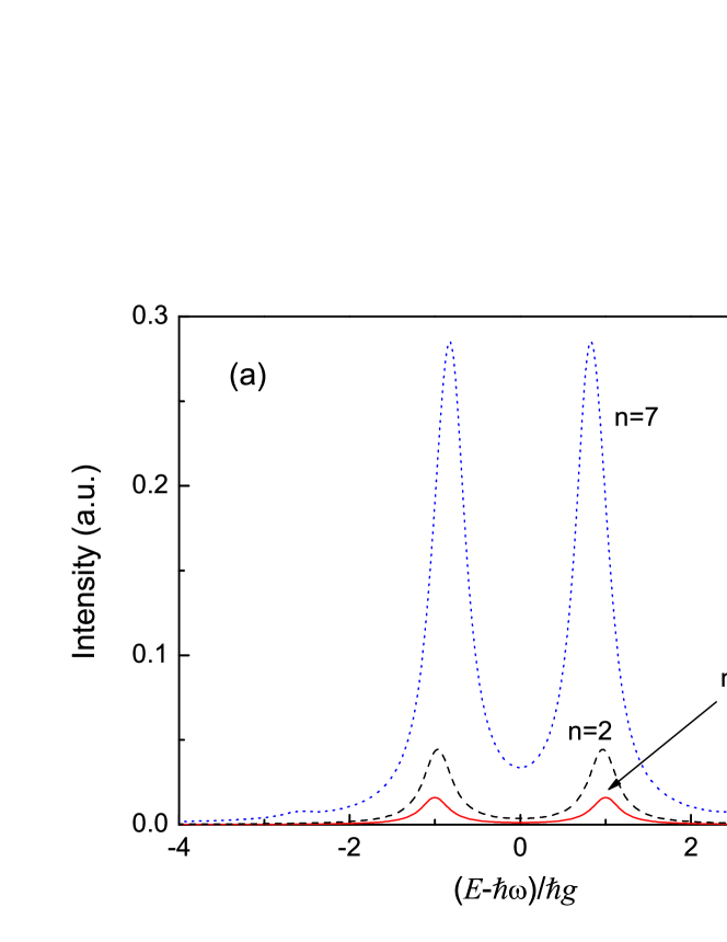
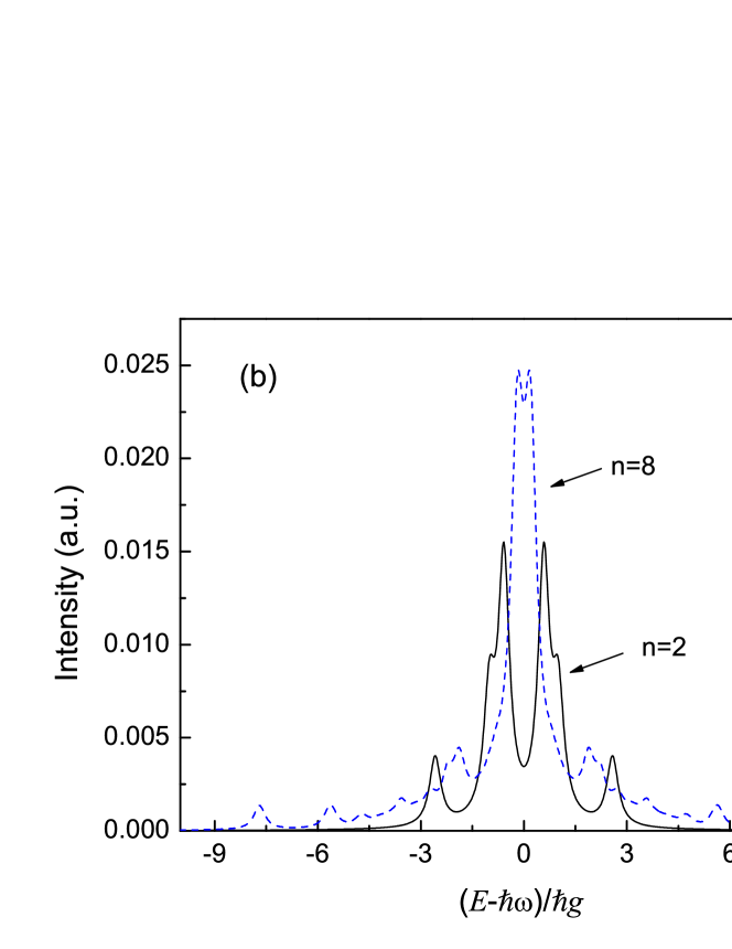
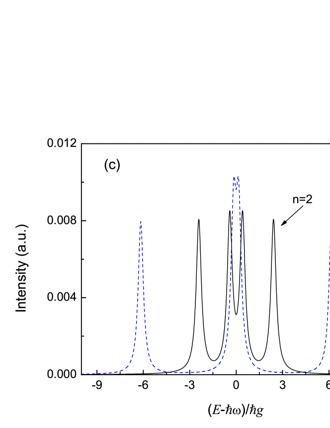
Figure 6: (Color online) Spectra for various intensities of the light field at specific values of $\gamma_{eh}$: (a) close to the bosonic limit with $\gamma_{eh}=-1.9\sqrt{\gamma_{e}\gamma_{h}}$ for $n=1$ (solid red), $2$ (dashed blue) and $7$ (dotted black) featuring a broadened and red-shifted Rabi doublet as the intensity increases and the onset of a multiplet structure, (b) intermediate case: $\gamma_{eh}=-\sqrt{\gamma_{e}\gamma_{h}}$ for $n=2$ (solid black) and $10$ (dashed blue) demonstrating a complicated multiplet structure and (c) close to the fermionic case with $\gamma_{eh}=-0.05\sqrt{\gamma_{e}\gamma_{h}}$ for $n=2$ (solid black) and $10$ (dashed blue) featuring quadruplet structure going towards Mollow triplet at high intensities.

Having demonstrated how our model interpolates between Fermi and Bose statistics, we now investigate in further detail the intermediate regime, by following the evolution of a single manifold between the two limits. In Fig. 7 the eigenvalues are displayed for the $7$th manifold, also shown on Fig. 1 for bosons and fermions. Eigenvalues are plotted as a function of $\gamma_{eh}$ running from $-2\sqrt{\gamma_{e}\gamma_{h}}$, which recovers the left hand side of Fig. 1, to $0$, which recovers the right hand side. Other manifolds behave in qualitatively the same way. In all cases, the $n+1$ equally spaced energies of the dressed bosons link to the two energies of the dressed fermions as follows: the upper energy $\mu\hbar\omega+\mu\hbar g$ of the Bose limit links to the upper energy $\mu\hbar\omega+\sqrt{\mu}\hbar g$ of the Fermi limit, and the symmetric behaviour occurs with the lower limit, linking $\mu\hbar\omega-\mu\hbar g$ with $\mu\hbar\omega-\sqrt{\mu}\hbar g$. More interestingly, the intermediate energies degenerate from the equal spacing of the Bose limit towards $\mu\hbar\omega$ near the Fermi limit, with a discontinuity when $\alpha_{2}$ becomes zero and only two eigen-energies remain. Physically, this discontinuity arises because for any $\gamma_{eh}\neq 0$, formally, an infinite number of excitations can be fitted in the QD, i.e. $\alpha_{n}$ never becomes exactly zero, see Fig. 4. With $\gamma_{eh}$ approaching zero these modes couple to light more and more weakly, thus the energies of the dressed states become close to the bare energy $\mu\hbar\omega$. When $\gamma_{eh}=0$ the fermionic regime is recovered and only two dressed eigenstates with energies $\mu\hbar\omega\pm\sqrt{\mu}\hbar g$ survive.

Figure 7: Energy diagram of the dressed excitons over the interval $\gamma_{eh}\in[-2\sqrt{\gamma_{e}\gamma_{h}},0]$ for the 7th manifold. The extremal values recover the diagrams of Fig. 1 with $n+1$ equally spaced energy levels in $n$th dressed boson manifold (far left) and twofold energy diagram with square root splitting for dressed fermions (far right). The two outer boson energies connect smoothly to the two fermion energies while the $n-1$ other one degenerate into a central line which disappears right when the system hits the Fermi limit (this point, $\gamma_{eh}=0$, is shown by circle).

Although the eigenvalue structure of the dressed excitons in the general case is simple and uniform, as is seen in Fig. 7, the multiplet structures which arises from it is, as has been seen in the spectra previously investigated, rich and varied. In the general case where $-2\sqrt{\gamma_{e}\gamma_{h}}<\gamma_{eh}<0$, two adjacent manifolds contain respectively $n+1$ and $n$ levels, transitions between any pair of which are possible. One may expect $n(n+1)$ lines in the emission spectra with a range of intensities and positions. The phenomenological broadening we have introduced leads to the decrease of the number of resolvable lines. In all cases the $n=1$ to $n=0$ transition provides only two lines, with constant energies throughout, because with only one exciton present the question of bosonic or fermionic behaviour is irrelevant. To access the consequences of exciton statistics, one must, unsurprisingly, reach higher manifolds.

In Fig. 8 we show the evolution of the spectra between the boson and fermion limits. They two panels are different projections of the same data, namely the multiplet structure as a function of $\gamma_{eh}\in[-2\sqrt{\gamma_{e}\gamma_{h}},0]$ for $n=12$. The Rabi doublet is seen to evolve into a Mollow triplet going through a complex and intertwined set of peaks whose splitting and relative heights vary with the value of $\gamma_{eh}$ considered. The spectrum obtained is therefore a direct probe of the underlying exciton quantum statistics.

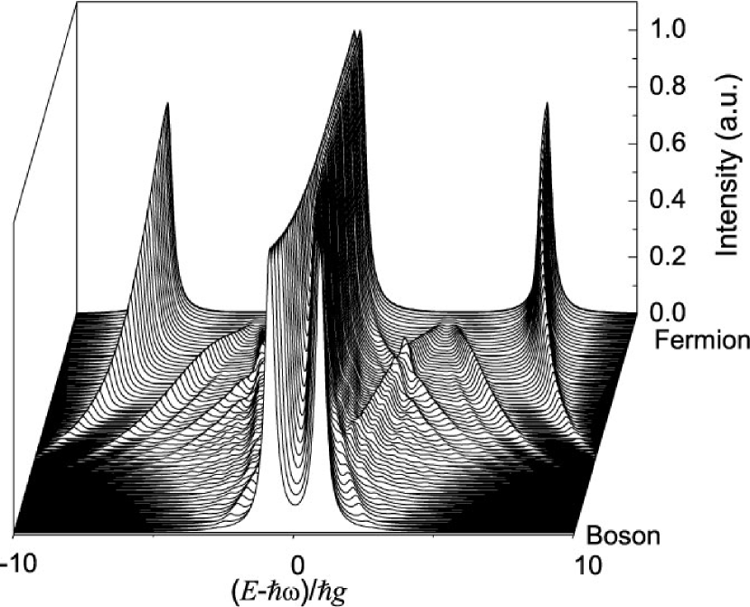
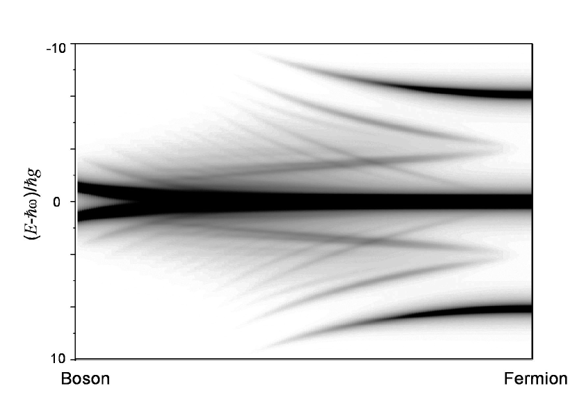
Figure 8: Transition from Fermi to Bose limits as observed in the optical emission spectra. (a) Superpositions of spectra for $\gamma_{eh}=-2\sqrt{\gamma_{e}\gamma_{h}}$ in front of the figure to $\gamma_{eh}=0$ at the back, recovering respectively the Rabi doublet and Mollow triplet. In the intermediate region, intricate and rich patterns of peaks appear, split, merge, or disappear. (b) Same data as in (a), but as a density plot on logarithmic scale, to discriminate the peaks, their positions and splitting as well as their relative intensities. All spectra are normalized to maximum intensity equal to $1$.

As a final comment, we note that if Eq. (46) was to hold for all $n$, it would yield, apart from a renormalization by $\sqrt{N}$, the Dicke model Dicke (1954), which has been widely used to describe various strong light-matter coupling phenomena Eastham and Littlewood (2001); Keeling et al. (2004). In our model it is recovered when $\beta_{m}=1/N^{(m-1)}$, a case that we have investigated in Ref. [Laussy et al., 2005].

At the heart of Dicke model lies the creation operator $J_{+}$ for an excitation of the “matter field” which distributes the excitation throughout the assembly of $N$ identical two-levels systems described by fermion operators $\sigma_{i}$, so that $b^{\dagger}$ in Eq. (2) maps to $J_{+}$ with

$$J_{+}=\sum_{i=1}^{N}\sigma_{i}^{\dagger}$$ (57)

One checks readily that $J_{+}$ and $J_{-}={J_{+}^{\dagger}}$ thus defined obey an angular momentum algebra with magnitude $N(N+1)$ (and maximum $z$ projection of $J_{z}$ equal to $N$). In this case the Rabi doublet arises in the limit where the total number of excitations $\mu$ (shared between the light and the matter field) is much less than the number of atoms, $\mu\ll N$, in which case the usual commutation relation $[J_{-},J_{+}]=-2J_{z}$ becomes $[J_{-}/\sqrt{N},J_{+}/\sqrt{N}]\approx 1$, which is the commutation for a bosonic field. This comes from the expression of a Dicke state with $\mu$ excitations shared by $N$ atoms given as the angular momentum state $\left|-N/2+\mu\right\rangle$. Therefore the annihilation/creation operators $J_{-}$, $J_{+}$ for one excitation shared by $N$ atoms appear in this limit like renormalised bose operators $\sqrt{N}a$, $\sqrt{N}{a^{\dagger}}$, resulting in a Rabi doublet of splitting $2\hbar g\sqrt{N}$. Such a situation corresponds, e.g., to an array of small QDs inside a microcavity such that in each dot electron and hole are quantized separately, while our model describes a single QD which can accommodate several excitons. The corresponding emission spectra are close to those obtained here below the saturation limit $\mu\ll N$, while the nonlinear regime $N\gg 1$, $\mu\gg 1$ has peculiar behaviour, featuring non-lorentzian emission line shapes and a non-trivial multiplet structure, like the “Dicke fork”. Laussy et al. (2005)

VI Conclusions and Prospects

The spectrum of light emitted by quantum dot excitons in leaky modes of a microcavity—which could be typically lateral emission—is a signature of the quantum statistics of excitons. A multiplet structure has been theoretically predicted with various features which can help identify the exciton field statistics. We provided the formalism to obtain the spectra expected for a general dot in various geometries based on the form of the single exciton wavefunction. We investigated a generic case analytically through a Gaussian approximation. The richness and specificity of the resulting spectra provides a means to determine, through the peak splittings and strength ratios, the parameter $\gamma_{eh}$ that measures how close excitons are to ideal fermions or bosons. Although heavy numerical computations are required for realistic structures, physical sense motivates that in small dots a Fermi-like behaviour of excitations with separately quantised electrons and holes is expected, while in larger dots behaviour should converge towards the Bose limit. These trends should be observable in the nonlinear regime (where more than one exciton interacts at a single time with the radiation mode): depending on whether Rabi splitting is found, or if a Mollow triplet or a more complicated multiplet structure arises, one will be able to characterize the underlying structure of the exciton field.

We have left the discussion of the interaction between excitons out of the scope of the present paper considering the effects which arise solely from Pauli exclusion principle. The effect of interactions, through screening of Coulomb potential by the electron-hole pairs, has been discussed in Refs. [Rombouts et al., 2005; Tanguy, 2002]. These papers demonstrate that the interactions will make fermionic behaviour more pronounced, since presence of other excitons screens the Coulomb interaction which binds electron and hole and leads to the increase of the Bohr radius. The question whether interactions will predominate over Pauli exclusion lies beyond the scope of this paper and we postpone it for a future work. Our preliminary estimations show that even at moderate excitonic density the effect of screening is small and does not lead to strong qualitative deviations.

To summarise, we have studied the effect of Pauli exclusion on the optical emission spectra of microcavities with embedded QDs in the strong coupling regime. We derived general expressions for the exciton creation operator which allow systematic computation of the light-matter coupling. The crossover between bosonic behaviour—observed in large QDs as Rabi doublet—to the fermionic behaviour—observed in small QDs as Mollow triplet—has been demonstrated.