Fractional charge in the noise of Luttinger liquid systems

Abstract

The current noise of a voltage biased interacting quantum wire adiabatically connected to metallic leads is computed in presence of an impurity in the wire. We find that in the weak backscattering limit the Fano factor characterizing the ratio between shot noise and backscattering current crucially depends on the noise frequency $\omega$ relative to the ballistic frequency $v_{F}/gL$, where $v_{F}$ is the Fermi velocity, $g$ the Luttinger liquid interaction parameter, and $L$ the length of the wire. In contrast to chiral Luttinger liquids, the noise is not only due to the Poissonian backscattering of fractionally charged quasiparticles at the impurity, but also depends on Andreev-type reflections of plasmons at the contacts, so that the frequency dependence of the noise needs to be analyzed to extract the fractional charge $e^{*}=eg$ of the bulk excitations. We show that the frequencies needed to see interaction effects in the Fano factor are within experimental reach.

1 INTRODUCTION

Shot noise measurements are a powerful tool to observe the charge of elementary excitations of interacting electron systems. This is due to the fact that in the Poissonian limit of uncorrelated backscattering of quasiparticles from a weak impurity, the low frequency current noise is directly proportional to the backscattered charge [1]. This property turns out to be particularly useful in probing the fractional charge of excitations in one-dimensional (1D) electronic systems, where correlation effects destroy the Landau quasiparticle picture and give rise to collective excitations, which in general obey unconventional statistics, and which have a charge different from the charge $e$ of an electron [2]. In particular, for fractional quantum Hall (FQH) edge state devices, which at filling fraction $\nu=1/m$ ($m$ odd integer) are usually described by the chiral Luttinger liquid (LL) model, it has been predicted that shot noise should allow for an observation of the fractional charge $e^{*}=e\nu$ of backscattered Laughlin quasiparticles [3]. Indeed, measurements at $\nu=1/3$ performed by two groups at the Weizmann Institute in Israel [4] and at the CEA-Saclay in France [5] have essentially confirmed this picture.

The question arises whether similar results can be expected also for non-chiral LLs, which are believed to be realized in carbon nanotubes [6] and single channel semiconductor quantum wires [7]. Although a non-chiral LL can be modelled through the very same formalism as a pair of chiral LLs, some important differences between these two kinds of LL systems have to be emphasized. In particular, in chiral LL devices right- and left-moving charge excitations are spatially separated, so that their chemical potentials can be independently tuned in a multi-terminal Hall bar geometry. In contrast, in non-chiral LL systems, right- and left-movers are confined to the same channel, and it is only possible to control the chemical potentials of the Fermi liquid reservoirs attached to the 1D wire. This in turn affects the chemical potentials of the right- and left-moving charge excitations in a non-trivial way depending on the interaction strength, and implies crucial differences between chiral and non-chiral LLs, for instance, the conductance in the former case depends on the LL parameter $g=\nu$ [8], while in the latter case it is independent of $g$ [9, 10, 11]. Hence, the predictions on shot noise properties of FQH systems can not be straightforwardly generalized to the case of non-chiral LLs, which therefore deserve a specific investigation. Previous theoretical calculations of the shot noise of non-chiral LL systems have shown that, even in the weak backscattering limit, the zero frequency noise of a finite-size non-chiral LL does not contain any information about the fractional charge backscattered off an impurity [12, 13], but is rather proportional to the charge of an electron. This result, as well as the above mentioned interaction independent DC conductance, prevents easy access to the interaction parameter $g$.

On the other hand, a quantum wire behaves as an Andreev-type resonator for an incident electron, which is transmitted as series of current spikes [9]. The reflections of charge excitations at both contacts are called Andreev-type reflections because they are momentum conserving as ordinary Andreev reflections [9, 14]. Since the transmission dynamics in the Andreev-type resonator depends on $g$, finite frequency transport can resolve internal properties of the wire. This is, in fact, the case for the AC conductance [9, 11, 15]. However, finite frequency conductance measurements are limited in the AC frequency range since the frequency must be low enough to ensure quasi-equilibrium states in the reservoirs in order to compare experiments to existing theories. The better alternative is to apply a DC voltage and measure finite frequency current noise. Exploring the out of equilibrium regime, we have recently shown that the noise induced by an impurity as a function of frequency has a periodic structure with period $2\pi\omega_{L}$, where $\omega_{L}=v_{F}/gL$ is the inverse of the traversal time of a charge excitation with plasmon velocity $v_{F}/g$ through the wire of length $L$ [16]. The Fano factor oscillates, and we demonstrate that by averaging over $2\pi\omega_{L}$, the effective charge $e^{*}=eg$ can be extracted from noise data. The interplay between the Andreev-type reflections and the backscattering of charge excitations at the impurity yields, in fact, many interesting phenomena both for the DC current as well as the finite frequency noise. As far as the DC current is concerned, the most remarkable feature is the appearance of oscillations as a function of $eV/\hbar\omega_{L}$, where $V$ is the applied voltage bias [17]. For the finite frequency excess noise, we have found regions of negativity showing interesting patterns which dramatically depend on the electron-electron interaction strength in the wire and are fundamentally different from their non-interacting counterparts [18].

2 Inhomogeneous Luttinger liquid model

In order to analyze the noise of non-chiral LLs, it is useful to study the inhomogeneous LL model, schematically illustrated in Fig. 1, which takes the finite length of the interacting wire and the adiabatic coupling to the Fermi liquid leads explicitly into account [9, 10]. This model is governed by the Hamiltonian

$${\mathcal{H}}={\mathcal{H}}_{0}\,+\,{\mathcal{H}}_{B}\,+\,{\mathcal{H}}_{V}\;,$$ (1)

where ${\mathcal{H}}_{0}$ describes the interacting wire, the leads and their mutual contacts, ${\mathcal{H}}_{B}$ accounts for the electron-impurity interaction, and ${\mathcal{H}}_{V}$ represents the coupling to the electrochemical bias applied to the wire. Explicitly, the three parts of the Hamiltonian read

$${\mathcal{H}}_{0} = \frac{\hbar v_{F}}{2}\int_{-\infty}^{\infty}dx\left[\Pi^{2}+\frac{1}{g^{2}(x)}(\partial_{x}\Phi)^{2}\right]\,,$$ (2)

$${\mathcal{H}}_{B} = \lambda\cos{[\sqrt{4\pi}\Phi(x_{0},t)+2k_{F}x_{0}]}\;,$$ (3)

$${\mathcal{H}}_{V} = \int_{-\infty}^{\infty}\frac{dx}{\sqrt{\pi}}\,\mu(x)\,\partial_{x}\Phi(x,t)\;.$$ (4)

Here, $\Phi(x,t)$ is the standard Bose field operator in bosonization and $\Pi(x,t)$ its conjugate momentum density [19]. The Hamiltonian ${\mathcal{H}}_{0}$ describes the (spinless) inhomogeneous LL, which is known to capture the essential physics of a quantum wire adiabatically connected to metallic leads. The interaction parameter $g(x)$ is space-dependent and its value is 1 in the bulk of the non-interacting leads and $g$ in the bulk of the wire ($0<g<1$ corresponding to repulsive interactions). The variation of $g(x)$ at the contacts from 1 to $g$ is assumed to be smooth, i.e. to occur within a characteristic length $L_{c}$ fulfilling $\lambda_{F}\ll L_{c}\ll L$, where $\lambda_{F}$ is the electron Fermi wavelength. The specific form of the function $g(x)$ in the contact region is expected not to influence physical properties for all energy scales below $\hbar v_{F}/L_{c}$. A recent analysis performed on a lattice model version of the inhomogeneous LL has confirmed this hypothesis [20]. Since the energy regime $E\geq\hbar v_{F}/L_{c}$ goes beyond the interest of the present work , we shall, henceforth, adopt a step-like function, cf. Fig. 1.

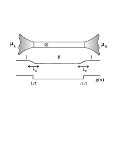
Figure 1: The upper part of the figure shows a quantum wire with an impurity adiabatically coupled to Fermi liquid leads. In order to allow for a finite bias, the leads are held on different electro-chemical potentials $\mu_{L}$ and $\mu_{R}$. The middle part of the figure shows the actual variation of the LL parameter $g$ along the wire-leads system in the inhomogeneous LL model, and the lower part of the figure its simplification under the assumption that $\lambda_{F}\ll L_{c}\ll L$.

The Hamiltonian ${\mathcal{H}}_{B}$ is the dominant $2k_{F}$ backscattering term at the impurity site $x_{0}$, and introduces a strong non-linearity in the field $\Phi$; the forward scattering term caused by the impurity has been omitted since it does not affect the statistics of the current. Finally, Eq. (4) contains the applied voltage. In most experiments leads are normal 2D or 3D contacts, i.e. Fermi liquids. However, since we are interested in properties of the wire, a detailed description of the leads would in fact be superfluous. One can account for their main effect, the applied bias voltage at the contacts, by treating them as non-interacting 1D systems ($g=1$), as mentioned above. The only essential properties originating from the Coulomb interaction that one needs to retain are (i) the possibility to shift the band-bottom of the leads, and (ii) electroneutrality [13]. Therefore, the function $\mu(x)$ appearing in Eq. (4), which describes the externally tunable electrochemical bias, is taken as piecewise constant $\mu(x<-L/2)=\mu_{L}$, $\mu(x>L/2)=\mu_{R}$ corresponding to an applied voltage $V=(\mu_{L}-\mu_{R})/e$. In contrast, the QW itself does not remain electroneutral in presence of an applied voltage, and its electrostatics emerges naturally from Eqs. (2)-(4) with $\mu=0$ for $|x|<L/2$ [11, 22].

3 Transport properties

In this section, we discuss the features of the average current and the current noise of the system depicted in Fig. 1. The former reads

$$I=\langle j(x,t)\rangle,$$ (5)

where the current operator is related to the Bose field $\Phi$ through $j(x,t)=-(e/\sqrt{\pi})\partial_{t}\Phi(x,t)$. Then, the latter, i.e. the finite frequency noise, is given by

$$S(x,y;\omega)=\int_{-\infty}^{\infty}dte^{i\omega t}\left\langle\left\{\Delta j(x,t),\Delta j(y,0)\right\}\right\rangle\;,$$ (6)

where $\{\,,\,\}$ denotes the anticommutator and $\Delta j(x,t)=j(x,t)-\langle j(x,t)\rangle$ is the current fluctuation operator. Since we investigate non-equilibrium properties of the system, the actual calculation of the averages of current and noise are performed within the Keldysh formalism [24].

The average current $I$ can be expressed as $I=I_{0}-I_{\rm BS}$, where $I_{0}=(e^{2}/h)V$ is the current in the absence of an impurity, and $I_{\rm BS}$ is the backscattering current. For arbitrary impurity strength, temperature, and voltage, the backscattering current can be written in the compact form

$$I_{\rm BS}(x,t)=-\frac{\hbar\sqrt{\pi}}{e^{2}}\int_{-\infty}^{\infty}dt^{\prime}\sigma_{0}(x,t;x_{0},t^{\prime})\langle j_{B}(x_{0},t^{\prime})\rangle_{\rightarrow}\ ,$$ (7)

where $\sigma_{0}(x,t;x_{0},t^{\prime})$ is the non-local conductivity of the clean wire [9, 11, 15]. In Eq. (7), we have introduced the “backscattering current operator”

$$j_{B}(x_{0},t)\equiv-\frac{e}{\hbar}\frac{\delta{\mathcal{H}}_{B}}{\delta\Phi(x_{0},t)}(\Phi+A_{0})\ ,$$ (8)

where $A_{0}(x_{0},t)$ is a shift of the phase field emerging when one gauges away the applied voltage. For a DC voltage this shift simply reads $A_{0}(x_{0},t)=\omega_{0}t/2\sqrt{\pi}$ with $\omega_{0}=eV/\hbar$ and $I_{\rm BS}$ does not depend on $x$ and $t$. Furthermore, we have introduced a “shifted average” $\langle\dots\rangle_{\rightarrow}$, which is evaluated with respect to the shifted Hamiltonian

$${\mathcal{H}}_{\rightarrow}={\mathcal{H}}_{0}[\Phi]+{\mathcal{H}}_{B}[\Phi+A_{0}]\;.$$ (9)

A straightforward though lengthy calculation shows that the finite frequency current noise (6) can (again for arbitrary impurity strength, temperature, and voltage) be written as the sum of three contributions

$$S(x,y;\omega)=S_{0}(x,y;\omega)+S_{A}(x,y;\omega)+S_{C}(x,y;\omega)\;.$$ (10)

The first part of Eq. (10), $S_{0}(x,y;\omega)$, is the current noise in the absence of a backscatterer, and can be related to the conductivity $\sigma_{0}(x,y;\omega)$ by the fluctuation dissipation theorem [25]

$$S_{0}(x,y;\omega)=2\hbar\omega\coth\left(\frac{\hbar\omega}{2k_{B}T}\right)\Re[\sigma_{0}(x,y;\omega)]\;.$$ (11)

The conductivity can be expressed by the Kubo formula $\sigma_{0}(x,y;\omega)=2(e^{2}/h)\omega C_{0}^{R}(x,y;\omega)$, where

$$C_{0}^{R}(x,y;\omega)=\int_{0}^{\infty}dte^{i\omega t}\langle[\Phi(x,t),\Phi(y,0)]\rangle_{0}$$ (12)

is the time-retarded correlator of the inhomogeneous LL model in the absence of an impurity. It is important to note that usually the relation (11) is only valid in thermal equilibrium, and the Kubo formula is based on linear response theory. However, due to the fact that in the absence of an impurity the current of a quantum wire attached to Fermi liquid reservoirs is linear in the applied voltage [9, 11], Eq. (11) is also valid out of equilibrium.

The other two terms in Eq. (10) arise from the partitioning of the current at the impurity site and reflect the statistics of the backscattering current. The second term is related to the anticommutator of the backscattering current operator $j_{B}$, and reads

$$S_{A}(x,y;\omega)=\frac{1}{\pi}\left(\frac{h}{2e^{2}}\right)^{2}\sigma_{0}(x,x_{0};\omega)f_{A}(x_{0},\omega)\sigma_{0}(x_{0},y;-\omega)$$ (13)

with

$$f_{A}(x_{0},\omega)=\int_{-\infty}^{\infty}dt\,e^{i\omega t}\left\langle\left\{\Delta j_{B}(x_{0},t),\Delta j_{B}(x_{0},0)\right\}\right\rangle_{\rightarrow}\;,$$ (14)

where $\Delta j_{B}(x,t)\equiv j_{B}(x,t)-\langle j_{B}(x,t)\rangle_{\rightarrow}$. Finally, the third part of Eq. (10) is related to the time-retarded commutator of $j_{B}$ and can be expressed as

$$S_{C}(x,y;\omega)=\frac{h}{2e^{4}\omega}\Bigl{\{}S_{0}(x,x_{0};\omega)f_{C}(x_{0},-\omega)\sigma_{0}(x_{0},y;-\omega)-S_{0}(y,x_{0};-\omega)f_{C}(x_{0},\omega)\sigma_{0}(x_{0},x;\omega)\Bigr{\}}$$ (15)

with

$$f_{C}(x_{0},\omega)=\int_{0}^{\infty}dt\left(e^{i\omega t}-1\right)\left\langle\left[j_{B}(x_{0},t),j_{B}(x_{0},0)\right]\right\rangle_{\rightarrow}\;.$$ (16)

The fractional charge is expected to emerge only in the limit of weak backscattering through the ratio between shot noise and backscattering current. We thus focus on the case of a weak impurity, retaining in the expressions (7) and (10) only contributions of second order in the impurity strength $\lambda$. Furthermore, we concentrate on the shot noise limit of large applied voltage $eV\gg\{k_{B}T,\hbar\omega,\hbar\omega_{L}\}$. Properties of the equilibrium current noise at finite frequency and temperature are discussed in detail in Ref. dolci05.

4 Fano factor

The backscattering current (7) may be written as $I_{\rm BS}=(e^{2}/h){\cal R}V$, where ${\cal R}$ is an effective reflection coefficient. Contrary to a non-interacting electron system, ${\cal R}$ depends on voltage and interaction strength [8, 17]. In the weak backscattering limit ${\cal R}\ll 1$, and its actual value can readily be determined from a measurement of the current voltage characteristics. Importantly, in the shot noise regime, i.e. for $eV\gg\{k_{B}T,\hbar\omega,\hbar\omega_{L}\}$, the noise can be shown to be dominated by the second term in Eq.(10) and to take the simple form [18]

$$S(x,x;\omega)\simeq 2eF(\omega)I_{\rm BS}\;,$$ (17)

where $x=y$ is the point of measurement (in either of the two leads). The Fano factor

$$F(\omega)=\frac{h^{2}}{e^{4}}|\sigma_{0}(x,x_{0};\omega)|^{2}$$ (18)

is given in terms of the non-local conductivity $\sigma_{0}(x,x_{0};\omega)$ relating the measurement point $x$ to the impurity position $x_{0}$, and reads explicitly

$$F(\omega)=(1-\gamma)^{2}\frac{1+\gamma^{2}+2\gamma\cos\left(\frac{2\omega(\xi_{0}+1/2)}{\omega_{L}}\right)}{1+\gamma^{4}-2\gamma^{2}\cos\left(\frac{2\omega}{\omega_{L}}\right)}\;.$$ (19)

The latter expression is, in fact, independent of the point of measurement $x$ and of temperature. On the other hand, it depends, apart from the frequency $\omega$, on the (relative) impurity position $\xi_{0}=x_{0}/L$, and the interaction strength through $\gamma=(1-g)/(1+g)$.

Figure 2: The periodic function $F(\omega)$, which determines the Fano factor, is shown as a function of $\omega/2\pi\omega_{L}$, for the case of an impurity at the center of the wire ($x_{0}=0$) and three different values of the interaction strength: $g=0.25$ (solid), $g=0.50$ (dashed), and $g=0.75$ (dotted). In the regime $\omega/\omega_{L}\ll 1$, the function tends to 1 independent of the value of $g$, but for $\omega\approx\omega_{L}$ the curve strongly depends on the interaction parameter $g$. In particular, $g$ can be obtained as the average over one period.

The result (17) shows that the ratio between the shot noise and the backscattering current crucially depends on the frequency regime one explores. In particular, for $\omega\rightarrow 0$, the function $F$ tends to 1, independent of the value of the interaction strength. Therefore, in the regime $\omega\ll\omega_{L}$ the observed charge is just the electron charge. In contrast, at frequencies comparable to $\omega_{L}$ the behavior of $F$ as a function of $\omega$ strongly depends on the LL interaction parameter $g$, and signatures of LL physics emerge. This is shown in Fig. 2 for the case of an impurity located at the center of the wire. Then, $F(\omega)$ is periodic, and the value at the minima coincides with $g^{2}$. Importantly, $g$ is also the mean value of $F$ averaged over one period $2\pi\omega_{L}$,

$$\left\langle S(x,x;\omega)\right\rangle_{\omega}\equiv\frac{1}{2\pi\omega_{L}}\int_{-\pi\omega_{L}}^{\pi\omega_{L}}S(x,x;\omega)\simeq 2egI_{\rm BS}\;,$$ (20)

where the approximation (17) has been used to describe $S(x,x;\omega)$. Seemingly, Eq. (20) suggests that quasiparticles with a fractional charge $e^{*}=eg$ are backscattered off the impurity in the quantum wire.

Let us discuss the physical origin of this appearance of fractional charge: We first consider the case of an infinitely long quantum wire. In the limit $L\to\infty$, i.e. $\omega_{L}\to 0$, $\xi_{0}\rightarrow 0$, the function $F(\omega)$ becomes rapidly oscillating and its average over any finite frequency interval approaches $g$. Hence, we recover in this limit the result for the homogeneous LL system [3], where the shot noise is directly proportional to the fractional charge $e^{*}=ge$ backscattered off the impurity. However, as shown above, the value of the fractional charge $e^{*}$ can be extracted not only in the borderline case $\omega\gg\omega_{L}$, but already for frequencies $\omega$ of order $\omega_{L}$. This is due to the fact that, although the contacts are adiabatic, the mismatch between electronic excitations in the leads and in the wire inhibits the direct penetration of electrons from the leads into the wire; rather a current pulse is decomposed into a sequence of fragments by means of Andreev-type reflections at the contacts [9]. These reflections are governed by the coefficient $\gamma=(1-g)/(1+g)$, which depends on the interaction strength. The zero frequency noise is only sensitive to the sum of all current fragments, which add up to the initial current pulse carrying the charge $e$. However, when $2\pi/\omega$ becomes comparable to the time needed by a plasmonic excitations to travel from the contact to the impurity site, the noise resolves the current fragmentation at the contacts. The sequence of Andreev-type processes is encoded in the non-local conductivity $\sigma_{0}(x,x_{0};\omega)$ relating the measurement point $x$ and the impurity position $x_{0}$. This enters into the Fano factor (18) and allows for an identification of $e^{*}$ from finite frequency noise data.

Figure 3: The Fano factor $F(\omega)$ is shown for the interaction strength $g=0.25$ and three different values of the (relative) impurity position $\xi_{0}=x_{0}/L$: $\xi_{0}=0$ (solid), $\xi_{0}=0.10$ (dashed), and $\xi_{0}=0.25$ (dotted). The combined effect of strong interactions and an off-centered impurity yields a very pronounced suppression of the Fano factor for certain noise frequencies.

When the impurity is located away from the center of the wire, $F(\omega)$ is no longer strictly periodic, as shown in Fig. 3. In that case, the combined effect of Coulomb interactions and an off-centered impurity can lead to a very pronounced reduction of the Fano factor for certain noise frequencies (see Fig. 3). Moreover, even if the impurity is off-centered, the detailed predictions (17) and (19) should allow to gain valuable information on the interaction constant $g$ from the low frequency behavior of the Fano factor determined by

$$F(\omega)=1-(1-g^{2})\Bigl{(}1+4g^{2}\xi_{0}(1+\xi_{0})\Bigr{)}\left(\frac{\omega L}{2v_{F}}\right)^{2}+{\cal O}\left(\frac{\omega}{\omega_{L}}\right)^{4}.$$ (21)

Finally, we would like to specify in more detail the parameter range for the validity of the relation (17). It turns out that the optimal voltage and temperature regime to extract (17) from the expression (10) for the full noise depends on the strength of the electronic correlations in the wire [18]. In Fig. 4, we illustrate two characteristic cases, namely $g=0.75$ (as appropriate for semiconductor quantum wires) and $g=0.25$ (as appropriate for metallic single-wall carbon nanotubes). The figure shows that the shot noise approximation (17) underestimates the full noise (10) even at large applied voltages. However, once a background noise

$$S_{\rm BG}=\frac{e^{2}}{\pi}\omega\coth\left(\frac{\hbar\omega}{2k_{B}T}\right)$$ (22)

has been subtracted from the full noise, which is done in order to obtain the (blue) dashed curve in Fig. 4, the approximation (17) and $S(x,x;\omega)-S_{\rm BG}$ agree within a few percent. The agreement becomes better the weaker the interactions. This is due to the fact that, in the weak interaction regime, the reflection coefficient of the Andreev-type processes is rather small and, therefore, the interference patterns in transport properties of the system are less pronounced.

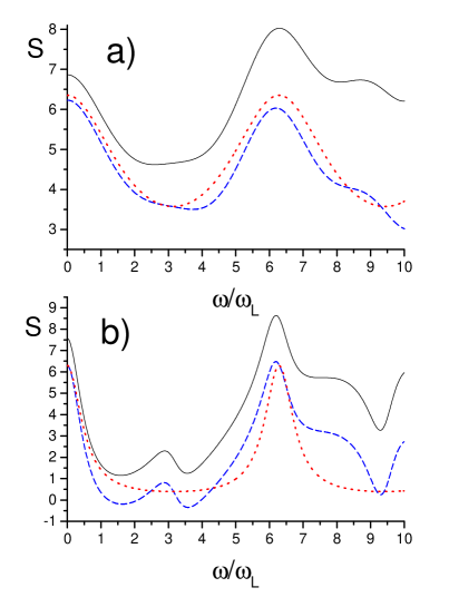
Figure 4: The frequency spectrum of the full noise $S(x,x;\omega)$, (black) solid line, in units of $e^{2}\omega_{L}$ and the approximation (17), (red) dotted line, are depicted for two systems with the parameters a) $g=0.75$, $k_{B}T/\hbar\omega_{L}=1$, $eV/\hbar\omega_{L}=100$, $\mathcal{R}=0.2$, and b) $g=0.25$, $k_{B}T/\hbar\omega_{L}=2$, $eV/\hbar\omega_{L}=98.83$, $\mathcal{R}=0.2$. The impurity is chosen at the center of the wire. The (blue) dashed curve resembles the full noise after a background subtraction, i.e. $S(x,x;\omega)-(e^{2}/\pi)\omega\coth(\hbar\omega/2k_{B}T)$.

5 Conclusions

The finite frequency noise of an interacting quantum wire coupled to Fermi liquid leads has been analyzed using the Keldysh technique for the inhomogeneous Luttinger liquid model. It has been shown that the interplay between pure interaction effects of the wire itself and the boundary effects at the crossover points between the wire and the leads results in non-trivial features of the transport properties of the system. The appearance of fractional charge $e^{*}=eg$ in the finite frequency noise of non-chiral LLs is solely due to a combined effect of backscattering of bulk quasiparticles at the impurity and of Andreev-type reflections of plasmons at the interfaces of wire and leads. The fractional charge $e^{*}$ can be extracted from the noise by averaging it over a frequency range of size $\pi\omega_{L}$ in the out of equilibrium regime. For single-wall carbon nanotubes we know that $g\approx 0.25$, $v_{F}\approx 10^{5}\;{\rm m/s}$, and their length can be up to 10 microns. Thus, we estimate $\pi\omega_{L}\approx 100\;{\rm GHz}\dots 1\;{\rm THz}$, which is a frequency range that seems to be experimentally accessible [26, 27]. Moreover, the requirement $eV\gg\hbar\omega_{L}$ should be fulfilled in such systems for $eV\approx 10\dots 50\;{\rm meV}$, a value which is well below the subband energy separation of about $1\;{\rm eV}$. Finally, we mention that similar oscillations as the ones predicted by us for the Fano factor of the finite frequency noise of a quantum wire with an impurity have recently been reported for the noise of a setup in which an STM tip allows for electron tunneling into a clean interacting quantum wire. [28]

- [1] Y. M. Blanter and M. Büttiker, Phys. Rep. 336, 1 (2000).
- [2] K.-V. Pham, M. Gabay, and P. Lederer, Phys. Rev. B 61, 16397 (2000).
- [3] C. L. Kane and M. P. A. Fisher, Phys. Rev. Lett. 72, 724 (1994).
- [4] R. de Picciotto, M. Reznikov, M. Heiblum, V. Umansky, G. Bunin, and D. Mahalu, Nature (London) 389, 162 (1997).
- [5] L. Saminadayar, D. C. Glattli, Y. Jin, and B. Etienne, Phys. Rev. Lett. 79, 2526 (1997).
- [6] M. Bockrath, D. H. Cobden, J. Lu, A. G. Rinzler, R. E. Smalley, L. Balents, and P. L. McEuen, Nature (London) 397, 598 (1999).
- [7] A. Yacoby, H. L. Störmer, K. W. Baldwin, L. N. Pfeiffer, and K. W. West, Phys. Rev. Lett. 77, 4612 (1996).
- [8] C. L. Kane and M. P. A. Fisher, Phys. Rev. B 46, 15233 (1992).
- [9] I. Safi and H. J. Schulz, Phys. Rev. B 52, R17040 (1995); Phys. Rev. B 59, 3040 (1999).
- [10] D. Maslov and M. Stone, Phys. Rev. B 52, R5539 (1995); V. V. Ponomarenko, Phys. Rev. B 52, R8666 (1995).
- [11] I. Safi, Ann. de Phys. (Paris) 22, 463 (1997); Eur. Phys. J. B 12, 451 (1999).
- [12] V. V. Ponomarenko and N. Nagaosa, Phys. Rev. B 60, 16865 (1999).
- [13] B. Trauzettel, R. Egger, and H. Grabert, Phys. Rev. Lett. 88, 116401 (2002).
- [14] N. P. Sandler, C. de C. Chamon, and E. Fradkin, Phys. Rev. B 57, 12324 (1998).
- [15] Ya. M. Blanter, F. W. J. Hekking, and M. Büttiker, Phys. Rev. Lett. 81, 1925 (1998).
- [16] B. Trauzettel, I. Safi, F. Dolcini, and H. Grabert, Phys. Rev. Lett. 92, 226405 (2004).
- [17] F. Dolcini, H. Grabert, I. Safi, and B. Trauzettel, Phys. Rev. Lett. 91, 266402 (2003).
- [18] F. Dolcini, B. Trauzettel, I. Safi, and H. Grabert, Phys. Rev. B. 71, 165309 (2005).
- [19] A. O. Gogolin, A. A. Nersesyan, and A. M. Tsvelik, Bosonization and Strongly Correlated Systems (Cambridge University Press, Cambridge, 1998).
- [20] T. Enss, V. Meden, S. Andergassen, X. Barnabe-Theriault, W. Metzner, and K. Schönhammer, Phys. Rev. B. 71, 155401 (2005).
- [21] T. Kleimann, F. Cavaliere, M. Sassetti, and B. Kramer, Phys. Rev. B 66, 165311 (2002).
- [22] R. Egger and H. Grabert, Phys. Rev. Lett. 77, 538 (1996); 80, 2255(E) (1998); 79, 3463 (1997).
- [23] B. Trauzettel and H. Grabert, Phys. Rev. B 67, 245101 (2003).
- [24] L. V. Keldysh, Sov. Phys. JETP 20, 1018 (1965); H. Kleinert, Path Integrals in Quantum Mechanics, Statistics, and Polymer Physics (World Scientific, Singapore, 1995).
- [25] V. V. Ponomarenko, Phys. Rev. B 54, 10328 (1996).
- [26] R. J. Schoelkopf, P. J. Burke, A. A. Kozhevnikov, D. E. Prober, and M. J. Rooks, Phys. Rev. Lett. 78, 3370 (1997).
- [27] R. Deblock, E. Onac, L. Gurevich, and L. P. Kouwenhoven, Science 301, 203 (2003).
- [28] A. V. Lebedev, A. Crépieux, and T. Martin, Phys. Rev. B. 71, 075416 (2005).