Cooper pairing and superconductivity on a spherical surface: applying the Richardson model to a multielectron bubble in liquid helium

Abstract

Electrons in a multielectron bubble in helium form a spherical, two-dimensional system coupled to the ripplons at the bubble surface. The electron-ripplon coupling, known to lead to polaronic effects, is shown to give rise also to Cooper pairing. A Bardeen-Cooper-Schrieffer (BCS) Hamiltonian arises from the analysis of the electron-ripplon interaction in the bubble, and values of the coupling strength are obtained for different bubble configurations. The BCS Hamiltonian on the sphere is analysed using the Richardson method. We find that although the typical ripplon energies are smaller than the splitting between electronic levels, a redistribution of the electron density over the electronic levels is energetically favourable as pairing correlations can be enhanced. The density of states of the system with pairing correlations is derived. No gap is present, but the density of states reveals a strong step-like increase at the pair-breaking energy. This feature of the density of states should enable the unambiguous detection of the proposed state with pairing correlations in the bubble, through either capacitance spectroscopy or tunneling experiments, and allow to map out the phase diagram of the electronic system in the bubble.

I Introduction

Spherical shells of charge carriers appear in a multitude of systems, such as multielectron bubbles in liquid helium VolodinJETP26 , metal nanoshells coating a non-conducting nanograin AverittPRL78 , carbon cages and fullerenes. Although the properties of flat two-dimensional systems have been widely studied, revealing new physics, the properties of spherical two-dimensional systems are much less well-studied. In this paper, we investigate the possibility and the properties of Cooper pairing in the spherical geometry.

The particular spherical two-dimensional system that we focus on is the multielectron bubble in liquid helium. When a flat surface of helium is charged with electrons above a critical charge density, an instability occurs with the surface opening to subsume a large number of electrons forming a bubble. These multielectron bubbles (MEBs) are typically micron-sized cavities inside liquid helium, containing a nanometer thin film of electrons on the inner surface of the bubble. The cavity is forced open by the Coulomb repulsion of the electrons which is balanced by the surface tension of the helium. The equilibrium shape of the bubble is spherical, with a radius $R$ determined by the number of electrons and the pressure on the helium.

The bare single electron states on the surface of the spherical bubble are angular momentum eigenstates and have discrete energies, characterized by the angular momentum $L$ and with degeneracy $2L+1$. At low temperature there will be a well defined Fermi surface located at the highest occupied state. Small-amplitude shape oscillations, including surface waves, can be quantized as spherical ripplons. The electrons can interact with these ripplons, and we will show that this leads to an attractive effective interaction between electrons.

This paper has two distinct but interwoven parts. In the first part (section II) we discuss in detail how the interactions between electrons and ripplons in the bubble can lead to a Cooper pairing scenario. The goal of the first part is to show that a BCS-type Hamiltonian provides a plausible description of the electronic system in multielectron bubbles at low temperatures, and to illustrate the relevant values of the parameters of the model Hamiltonian. In the second part (sections III-IV) we investigate the general properties of this Hamiltonian using the Richardson solution for the reduced BCS Hamiltonian describing pairing e.g. in nanograins. Both the ground state properties and the density of states of a spherical two-dimensional BCS system, are derived and discussed.

II Cooper pairs on a spherical surface

First, we investigate the three ingredients of the full Hamiltonian: the electronic part, the ripplonic part, and the electron-ripplon coupling. Then, we analyze the effective interaction between electrons, resulting from both the Coulomb interactions and the ripplon-mediated electron-electron interaction. Finally, we arrive at a BCS-type Hamiltonian for the multielectron bubble.

II.1 Electrons and ripplons in the bubble

The spherical 2D electron system – The well-known Hamiltonian of interacting electrons in a flat 2D electron gas (2DEG) in the jellium model can be written in second quantization as

$$\hat{H}_{\text{e}}^{\text{flat}} =\sum_{\mathbf{k},\sigma}\epsilon_{k}\hat{c}_{\mathbf{k},\sigma}^{{\dagger}}\hat{c}_{\mathbf{k},\sigma}$$

$$+\sum_{\mathbf{q}>0}\sum_{\mathbf{k},\sigma}\sum_{\mathbf{k}^{\prime},\sigma^{\prime}}v_{q}\hat{c}_{\mathbf{k}+\mathbf{q},\sigma}^{{\dagger}}\hat{c}_{\mathbf{k}^{\prime}-\mathbf{q},\sigma^{\prime}}^{{\dagger}}\hat{c}_{\mathbf{k}^{\prime},\sigma^{\prime}}\hat{c}_{\mathbf{k},\sigma}.$$ (1)

where $\hat{c}_{\mathbf{k},\sigma}^{{\dagger}}\hat{c}_{\mathbf{k},\sigma}$ create and destroy an electron with wave number $\mathbf{k}$ and spin $\sigma$, and

$$\epsilon_{k}=\frac{\hbar^{2}}{2m_{\text{e}}}k^{2},\text{ }v_{k}=\frac{e^{2}}{2\varepsilon A}\frac{1}{k}$$ (2)

where $m_{\text{e}}$ is the electron mass, $A$ is the surface of the 2D system, $\varepsilon$ is the permittivity of the medium and $e$ is the electron charge.

The Hamiltonian of the interacting spherical electronic system has a very similar form, provided that one uses spherical harmonics $Y_{L,m}(\theta,\phi)$ instead of plane waves as the single-particle basis functions. For this purpose we use the operators $\hat{c}_{L,m}^{{\dagger}}$ and $\hat{c}_{L,m}$ that create, resp., annihilate an electron in the angular momentum eigenstate $(L,m)$, i.e. $\psi_{L,m}(\theta,\phi)=Y_{L,m}(\theta,\phi)$. The Hamiltonian of the interacting spherical two-dimensional electron gas (S2DEG) becomes

$$\hat{H}_{\text{e}}^{\text{sphere}} =\sum_{L,m,\sigma}\epsilon_{L}\hat{c}_{L,m,\sigma}^{{\dagger}}\hat{c}_{L,m,\sigma}$$

$$+\sum_{J>0,n}\sum_{L,m,\sigma}\sum_{L^{\prime},m^{\prime},\sigma}v_{L}\hat{c}_{(L,m)\otimes(J,n),\sigma}^{{\dagger}}\hat{c}_{(L^{\prime},m^{\prime})\otimes(J,-n),\sigma^{\prime}}^{{\dagger}}\hat{c}_{L^{\prime},m^{\prime},\sigma^{\prime}}\hat{c}_{L,m,\sigma}$$ (3)

where we use the notation $\sum_{L,m}=\sum_{L=0}^{\infty}\sum_{m=-L}^{L}$ and

$$\epsilon_{L}=\frac{\hbar^{2}}{2m_{\text{e}}}\frac{L(L+1)}{R^{2}}\text{, }v_{L}=\dfrac{e^{2}}{2\varepsilon R}\dfrac{(-1)^{L}}{2L+1},$$ (4)

where $R$ is the radius of the sphere. The typical scale of the kinetic energy $\epsilon_{1}=\hbar^{2}/(m_{\text{e}}R^{2})$ is listed for several bubble sizes and pressures in table I. The operator $\hat{c}_{(L,m)\otimes(J,n),\sigma}^{+}$ creates a spin $\sigma$ electron in a single particle state resulting from adding the angular momenta $(L,m)$ and $(J,n).$ Formally, we have

$$\begin{array}[c]{c}\hat{c}_{(L,m)\otimes(J,n),\sigma}^{+}={\displaystyle\sum\limits_{L^{\prime}=|L-J|}^{L+J}}{\displaystyle\sum\limits_{m^{\prime}=-L^{\prime}}^{L^{\prime}}}\sqrt{\dfrac{(2L+1)(2J+1)}{4\pi(2L^{\prime}+1)}}\left\langle J,0;L,0|L^{\prime},0\right\rangle\\ \times\text{ }\left\langle J,n;L,m|L^{\prime},m^{\prime}\right\rangle\text{ }\hat{c}_{L^{\prime}m^{\prime},\sigma}^{+},\end{array}$$ (5)

where $\left\langle J,n;L,m|L^{\prime},m^{\prime}\right\rangle$ is the Clebsch-Gordan coefficient for combining the angular momenta $(L,m)$ and $(J,n)$ into a state of angular momentum $(L^{\prime},m^{\prime})$. The role of the momentum is now taken by the angular momentum. Indeed, taking $L/R\rightarrow k$ for large $L$ links the result for the spherical case to that for the flat case. This link was noted previously for the structure factor of the spherical 2D electron gas TemperePRB65 , and its response to a weak magnetic field.

When the Coulomb energy is small compared to the kinetic energy, the electrons fill up a Fermi sea of angular momentum states $L$ (with degeneracy $2L+1$) up to a Fermi level $L=L_{F}$. The level splitting at the Fermi level, $\Delta\epsilon=\epsilon_{L_{F}}-\epsilon_{L_{F}-1}$, is given in Table I for some typical bubbles. The typical value of the distance between electronic levels is THz (or mK).

Note that the $J=0$ term is absent in the Coulomb part of the Hamiltonian (3): this term is exactly cancelled by the surface tension energy of the helium as shown in Ref. TemperePHYSE22 . In Hamiltonian (1) for the flat 2D electron gas in jellium, the $\mathbf{q}=0$ term is absent because it is canceled by a homogeneous positive background introduced in the jellium model. Thus the surface tension energy in MEBs takes a role similar to the homogenous positive background in jellium.

Table 1: Several typical length and energy scales for the electron-ripplon system in the bubble are given in this table, for bubbles with different numbers of electrons and subjected to different pressures. The first row lists the bubble radius in microns. The second row lists the kinetic energy scale $\epsilon_{1}=\hbar^{2}/(m_{\text{e}}R^{2})$ of electrons in the bubble, the energy of angular momentum level $L$ being $\epsilon_{L}=\epsilon_{1}L(L+1)/2$. The third row gives the electronic level splitting $\Delta\epsilon=\epsilon_{1}(L_{F}+1)$, at the Fermi level, between the subsequent angular momentum levels of the spherical 2D electron gas. The fourth row lists the energy scale for ripplons, $\hbar\omega_{r}=\hbar[\sigma/(\rho R^{3})]^{1/2}$ in $\mu$K (1 $\mu$K corresponds to 0.1309 MHz). The fifth row gives the strength of the electric field at the bubble surface, pressing the electrons to the helium surface and resulting in electron-ripplon coupling. The sixth row provides values for the electron-ripplon coupling constant $g$ in expression (9).

		$N=10^{4}$			$N=10^{5}$			$N=10^{6}$
$p$ (Pa)	0	102	104	0	102	104	0	102	104
$R$ ($\mu$m)	1.062	.5236	.1709	4.937	1.6930	.5409	22.93	5.393	1.711
$\epsilon_{1}$ (mK)	.7836	3.225	30.27	.0363	.3084	3.022	1.68$\times$10-3	.0304	.3021
$\Delta\epsilon$ (mK)	55.64	229.0	2149.	8.127	69.10	673.0	1.191	21.53	213.9
$\hbar\omega_{r}$ ($\mu$K)	10.99	31.76	170.3	1.097	5.463	30.25	.1096	.9611	5.378
$\mathbf{E}$ (kV/cm)	63.80	262.6	2465.	29.54	251.2	2461.	13.70	247.6	2459.
$g$ (mK)	25.87	124.1	1909.	4.933	49.70	803.3	.9813	20.61	338.5

Ripplons on the bubble surface – Small-amplitude oscillations of the bubble surface can be quantized, leading to the concept of spherical ripplons. The ripplon gas (excluding the breathing mode) is described by the Hamiltonian

$$\hat{H}_{\text{ripl}}=\sum_{L>0,m}\hbar\omega_{L}\hat{a}_{L,m}^{+}\hat{a}_{L,m}.$$ (6)

The bare ripplonic frequencies for this system, at a pressure $p$, are TemperePRL87

$$\omega_{L}=\sqrt{\frac{\sigma}{\rho R^{3}}(L+1)(L^{2}+L+2)+\frac{p}{\rho R^{2}}2(L+1)},$$ (7)

where $\sigma=3.6\times 10^{-4}$ J/m² is the surface tension of helium, and $\rho=145$ kg/m³ is its density. In the surface tension dominated regime ($pR/\sigma<1$), $\omega_{L}=\omega_{r}L^{3/2}$ with $\omega_{r}=[\sigma/(\rho R^{3})]^{1/2}$. Typical ripplon frequencies lie in the MHz-GHz (or $\mu$K) range. The ripplon Green’s function is defined by

$$D(L,m;t) =-i\left\langle\mathcal{T}[\hat{A}_{L,m}(t)\hat{A}_{L,m}^{+}(0)]\right\rangle$$

$$\text{with }\hat{A}_{L,m}=\hat{a}_{L,m}+\hat{a}_{L,-m}^{+},$$

where $\mathcal{T}$ is the time ordering operator and $\hat{A}_{L,m}$ is a sum of ripplon creation and annihilation operators. The unperturbed ripplon propagator (corresponding to a system described by $\hat{H}_{\text{ripl}}$ above) in the frequency domain is

$$D^{(0)}(L,m;\omega)=\dfrac{2\hbar\omega_{L}}{(\hbar\omega)^{2}-(\hbar\omega_{L})^{2}+i\eta}.$$

where $\eta$ is a positive infinitesimal.

Electron-ripplon interaction – The electron-ripplon interaction can be written as

$$\hat{H}_{\text{int}}=\sum_{J,n}M_{J}\hat{A}_{J,n}\sum_{L,m,\sigma}\hat{c}_{(L,m)\otimes(J,n),\sigma}^{+}\hat{c}_{L,m,\sigma},$$ (8)

where $M_{J}$ is the electron-ripplon interaction amplitude and $\sum_{L,m,\sigma}\hat{c}_{(L,m)\otimes(J,n),\sigma}^{+}\hat{c}_{L,m,\sigma}$ is the $(J,n)$ spherical component of the electron density.

The interaction between the electrons and the ripplons comes about due to the presence of an electric field, generated by the electrons themselves and pressing the electrons against the helium surface. This is the electric pressing field $E=eN/(2R^{2})$, directed radially. When a ripplon is present, it moves the electrons in the electric field generated by all other electrons and this results in an interaction energy. The interaction energy is the product of the displacement caused by the ripplon and the electric field, summed for all electrons, similarly as in KliminSSC126 . Rewriting this interaction energy in second quantization operators, we find the interaction Hamiltonian (8) with the interaction amplitude

$$M_{J}=g\frac{(J+1/2)^{1/2}}{[(J+1)(J^{2}+J+2+2pR/\sigma)]^{1/4}},$$ (9)

where the coupling constant due to the pressing electric field $E$ (see Table I) is given by

$$g^{\text{(e)}}=\frac{1}{2\sqrt{\pi}}\frac{-eE}{R}\sqrt{\frac{\hbar}{2\rho R\omega_{r}}}.$$ (10)

An additional contribution to the interaction energy between electrons and ripplons can be derived as the change in polarization energy of the electron-helium system when the helium surface is deformed and the electrons are at rest. This mechanism for coupling was first derived by M. Cole ColePRB2 for electrons on a flat surface. Following the arguments of Cole, we obtain a similar expression for the interaction amplitude (9) but with a different coupling constant

$$g^{\text{(p)}}=\frac{9\sqrt{\pi}}{8}\frac{\varepsilon-1}{\varepsilon+1}\frac{e^{2}}{4\pi d^{2}R}\sqrt{\frac{\hbar}{2\rho R\omega_{r}}},$$ (11)

where $d$ is the expectation value for the distance between the electron and the helium surface. The total electron-ripplon coupling constant is then $g=g^{\text{(p)}}+g^{\text{(e)}}.$

A single electron coupled to a bath of ripplons forms a ripplonic polaron JacksonPRB24 . In a multielectron bubble, the electric field pressing the electrons against the helium surface can be much larger than the field achievable on a flat helium surface, so that the ripplonic polarons will be in the strong coupling regime, and can even form a Wigner lattice of ripplonic polarons TempereEPJB32 .

II.2 Effective electron-electron interaction

Cooper’s argument – In this subsection, we follow Cooper’s argument for pairing CooperPR104 and apply this to the present case of electrons and ripplons in the bubble. The effective electron-electron interaction is the sum of the Coulomb interaction between the electrons and a ripplon-mediated attractive interaction between the electrons. In TemperePRB65 we drew a Feynman diagram to represent the Coulomb interaction between the electrons. Now, we can add another diagram with the same electron propagator lines, but instead of exchanging a virtual photon, exchanging a virtual ripplon. This is shown in Fig. 1.

Figure 1: Electrons interact through the exchange of virtual photons or ripplons. The vertex contributions and propagator for both interactions are shown in this figure.

The two diagrams in Fig. 1 can be represented by a single diagram using an effective interaction

$$V_{\text{eff}}(L,m;\omega)=\dfrac{e^{2}}{2\varepsilon R}\dfrac{1}{2L+1}+M_{L}^{2}\dfrac{2\hbar\omega_{L}}{(\hbar\omega)^{2}-(\hbar\omega_{L})^{2}+i\eta}.$$ (12)

Both the Coulomb and the ripplon-exchange interaction are given by a product of two vertex factors and one virtual particle propagator. The total electron-electron interaction Hamiltonian can be written as

$$\hat{H}_{\text{int}}(t) =\sum_{L,m,\sigma}\sum_{L^{\prime},m^{\prime},\sigma^{\prime}}\sum_{J,n}\left[\int\frac{d\omega}{2\pi}V_{\text{eff}}(J,n;\omega)e^{i\omega t}\right]$$

$$\times(-1)^{n}\hat{c}_{(L,m)\otimes(J,n),\sigma}^{+}\hat{c}_{(L^{\prime},m^{\prime})\otimes(J,-n),\sigma^{\prime}}^{+}\hat{c}_{L^{\prime},m^{\prime},\sigma^{\prime}}\hat{c}_{L,m,\sigma}.$$

Let’s study for which regimes $V_{\text{eff}}(J,n;\omega)$ is attractive, i.e. for which values of $(J,n;\omega)$ the ripplonic part dominates and is attractive. It is clear that small energy transfers make the ripplonic part attractive because $D^{(0)}(L,\omega\rightarrow 0)=-2/(\hbar\omega_{L})$. Moreover, in general ripplon exchange will indeed occur with $\omega=0$. The reason for this is that the ripplonic energies are much smaller than the electronic level spacing, as can be seen from comparing rows 3 and 4 of table I. For ripplons with $L$ smaller than $\sim 10^{3}$, the absorption or emission of a ripplon with angular momentum $L$ cannot change the angular momentum of the electron due to energy conservation requirements. The effective interaction at $\omega=0$ is

$$V_{\text{eff}}(L,m;0)=\dfrac{e^{2}}{2\varepsilon R}\dfrac{1}{2L+1}-\dfrac{2M_{L}^{2}}{\hbar\omega_{L}}.$$ (13)

The attractive interaction dominates strongly at small $L,$ since $2g^{2}/(\hbar\omega_{r})\gg e^{2}/2\varepsilon R$ as can be checked for typical bubbles by substituting the values from Table I. It is strongest for small $L$ and decreases roughly as $L^{-2}$:

$$V_{\text{eff}}(L,m;0)\approx-\dfrac{2M_{L}^{2}}{\hbar\omega_{L}}=-\frac{2g^{2}}{\hbar\omega_{r}}\frac{(L+1/2)}{(L+1)(L^{2}+L+2+2pR/\sigma)}.$$ (14)

The strength of the effective interaction is $2g^{2}/(\hbar\omega_{\sigma})$. Since the $g$ is of the order of mK and $\hbar\omega_{r}$ of the order of $\mu$K (see Table I), the effective attractive interaction is large as compared the relevant energy scales $g$, $\hbar\omega_{r}$, and $\epsilon_{1}$. We are clearly in a strong coupling regime, in agreement with the results from TempereEPJB32 .

Intralevel pairing – Since the ripplon energies are much smaller than the electronic level spacing at the Fermi level, the attractive interaction only takes place between two electrons on the same angular momentum level, and these electrons will be scattered into final states also on that angular momentum level. An electron in angular momentum state $\left|\text{initial}\right\rangle=\left|L,m\right\rangle$, which emits a spherical ripplon in angular momentum state $\left|J,n\right\rangle$, finds itself in the following superposition of angular momentum states

$$\left|\text{final}\right\rangle =\sum_{L^{\prime}=|L-J|}^{L+J}\sqrt{\dfrac{(2L+1)(2J+1)}{4\pi(2L^{\prime}+1)}}\left\langle L,0;J,0|L^{\prime},0\right\rangle$$

$$\times\left\langle L,m;J,-n|L^{\prime},m-n\right\rangle\text{ }\left|L^{\prime},m-n\right\rangle.$$

The projection of this final state $\left|\text{final}\right\rangle$ on the angular momentum level $L$ of the initial state is

$$f_{CG}[(L,m),(J,-n)] =\sqrt{\dfrac{2J+1}{4\pi}}\left\langle L,0;J,0|L,0\right\rangle$$

$$\times\left\langle L,m;J,-n|L,m-n\right\rangle.$$

Thus, the scattering process between two electrons with spin $\sigma$ and $\sigma^{\prime}$ on the angular momentum level $L$ can be described in second quantization as

$$\hat{H}_{\text{int,}L} =\sum_{m=-L}^{L}\sum_{m^{\prime}=-L}^{L}\sum_{J,n}f_{CG}[(L,m),(J,-n)]f_{CG}[(L,m^{\prime}),(J,n)]$$

$$\times V_{\text{eff}}(J,n;0)\hat{c}_{L,m-n,\sigma}^{+}\hat{c}_{L,m^{\prime}+n,\sigma^{\prime}}^{+}\hat{c}_{L,m^{\prime},\sigma^{\prime}}\hat{c}_{L,m,\sigma}$$

This interaction Hamiltonian derived for the multielectron bubble is already close to a BCS-like interaction Hamiltonian. It involves only electrons on the same angular momentum level and couples them with an attractive potential.

An initial state with a pair characterized by $\{m,m^{\prime}\}$ can be scattered into a pair with $\{m-n,m^{\prime}+n\}$ in various ways: namely by the scattering of a virtual ripplon with $J=n,n+1,n+2,....$ provided that $J$ is an even mode to obey the triangle rule of addition of angular momenta. All these processes are indistinguishable (initial and final states are exactly the same) and their diagrams should be added to get the overall amplitude. Different combinations of Clebsch-Gordan coefficients will occur, which can take either a positive or a negative sign: the different diagrams can interfere constructively but also destructively. The only case where we are sure that the different contributions will interfere constructively, is for pairs of electrons with opposite angular momentum $m^{\prime}=-m$. The reason for this is that $\left\langle L,m;J,n|L,m+n\right\rangle$ has the same sign as $\left\langle L,-m;J,-n|L,-m-n\right\rangle$. We investigated this point numerically, and found that the total effective interaction is indeed strongly reduced for pairs that do not have opposite angular momentum ($m^{\prime}\neq-m$). However, for $m^{\prime}=m$ we find that the effective interaction potential is not reduced and is only weakly dependent on $m$.

Effective Hamiltonian – From the previous section we know that the interaction between the electrons can be written in the form of a BCS interaction Hamiltonian given by

$$\hat{H}_{\text{int}}=-\sum_{L}\sum_{m=-L}^{L}\sum_{m^{\prime}=-L}^{L}\tilde{V}_{m,m^{\prime},L}\text{ }\hat{c}_{L,-m^{\prime}\downarrow}^{+}\hat{c}_{L,m^{\prime};\uparrow}^{+}\hat{c}_{L,m;\uparrow}\hat{c}_{L,-m;\downarrow},$$ (15)

where $\sigma=$ $\uparrow,\downarrow$ denotes spin up and spin down and

$$\tilde{V}_{m,m^{\prime},L} =\sum_{J=\max[2,|m-m^{\prime}|]}^{2L}\frac{2g^{2}}{\hbar\omega_{\sigma}}\frac{(J+1/2)}{(J+1)(J^{2}+J+2+2pR/\sigma)}$$

$$\times f_{CG}[(L,m),(J,m^{\prime}-m)]f_{CG}[(L,-m),(J,m-m^{\prime})].$$ (16)

Due to the coefficients $\left\langle L,0;J,0|L,0\right\rangle$ the summation cannot run further than $2L$ and only even values of $J$ contribute. The summation starts from $n=|m-m^{\prime}|$, or if this is less than 2, it starts at $J=2$. The $J=0$ deformation is not taken into account (it is the radius of the bubble), and the $J=1$ deformation is a uniform translation which cannot couple to the internal degrees of freedom. To proceed, we will introduce an averaged interaction amplitude at the Fermi angular momentum level:

$$G=\frac{1}{(2L_{F}+1)^{2}}\sum_{m,m^{\prime}}\tilde{V}_{m,m^{\prime},L_{F}}.$$ (17)

The interaction amplitude still depends on the angular momentum level $L$. But, as we shall see in the next section, pair correlations occur only in levels close to $L_{F}$ where the $L$-dependence of the interaction amplitude can be neglected. So we use the value of the interaction amplitude at $L_{F}$ also for levels close to $L_{F}$. Values for $G$ for various configurations are given in Figure 2.

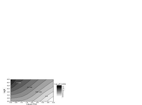
Figure 2: BCS interaction strength $G$ (in mK) as a function of pressure $p$ and number of electrons $N$ in the bubble.

With this, we have established that the properties of the ripplon-mediated electron-electron interaction lead to a Cooper-type attractive interaction between the electrons, and to a BCS-like Hamiltonian

$$\hat{H}_{\text{eff}} =\sum_{L,m,\sigma}\epsilon_{L}\hat{c}_{L,m;\sigma}^{+}\hat{c}_{L,m;\sigma}$$

$$-G\sum_{L}\sum_{m,m^{\prime}=-L}^{L}\hat{c}_{L,-m^{\prime}\downarrow}^{+}\hat{c}_{L,m^{\prime};\uparrow}^{+}\hat{c}_{L,m;\uparrow}\hat{c}_{L,-m;\downarrow}.$$ (18)

The peculiarity of this pairing Hamiltonian is that the pairing takes place within discrete energy levels. This effective Hamiltonian for electrons pairing due to an attractive interaction brought about by ripplon exchange can be solved by introducing a variational many body wave function as in the BCS treatment. However, we chose to apply the Richardson method RichardsonPL3 , initially developed in the context of nuclear physics and recently reintroduced vonDelftSSP39 to the condensed matter community to describe superconductivity in nanosize metallic grains. This method is particularly suitable for finite systems with a discrete level structure such as the multielectron bubble.

III Richardson model for pairing in a S2DEG

Having argued that multielectron bubbles are a suitable candidate to observe pairing of electrons in a spherical two-dimensional system, we will apply the Richardson model to the effective pairing Hamiltonian (18) to gain insight in the properties of the paired phase.

Note that the analysis here can be applied to the general problem of a S2DEG with attractive interactions between electrons on the same angular momentum level. The previous section provides possible values for the coupling constant $G$ (see Fig. 2) and for the relevant energy scales (see Table I), and a justification for the applicability of the effective pairing Hamiltonian (18) to multielectron bubbles specifically. Nevertheless the results derived in this section can be used to investigate other systems such as the superconducting properties of thin electronic nanoshells, or can be investigated as an academic question regarding spherical electronic systems.

III.1 Energy levels of interacting electrons

The Richardson model provides a method of solution for the so-called reduced BCS Hamiltonian vonDelftPRL77 ; MatveevPRL79 :

$$\hat{H}_{\text{BCS}}=\sum_{i,\sigma}\varepsilon_{i}\hat{b}_{i,\sigma}^{+}\hat{b}_{i,\sigma}-G\sum_{i,i^{\prime}}\hat{b}_{i^{\prime},\uparrow}^{+}\hat{b}_{i^{\prime},\downarrow}^{+}\hat{b}_{i,\downarrow}\hat{b}_{i,\uparrow}.$$ (19)

Now consider the Hamiltonian (18) that we derived in the previous section, and collect all terms that contain operators working on the angular momentum level $L$:

$$\hat{H}_{\text{L}} =\sum_{m,\sigma}\epsilon_{L}\hat{c}_{L,m;\sigma}^{+}\hat{c}_{L,m;\sigma}$$

$$-G\sum_{m,m^{\prime}=-L}^{L}\hat{c}_{L,-m^{\prime}\downarrow}^{+}\hat{c}_{L,m^{\prime};\uparrow}^{+}\hat{c}_{L,m;\uparrow}\hat{c}_{L,-m;\downarrow}.$$ (20)

Note that only electrons within the same angular momentum energy level $L$ interact: only intralevel interactions take place, but no interlevel interactions. This is due to the fact that the relevant ripplon energies are much smaller than the interlevel energy splitting (see Table I for typical values in multielectron bubbles). So, the set of electrons with a given angular momentum $L$ can be considered as an independent subsystem, described by the Hamiltonian (20). The full system is the collection of independent subsystems characterized by different $L$. The full Hamiltonian (18) is just the sum of the Hamiltonians (20) describing independent subsystems with different $L$ :

$$\hat{H}_{\text{eff}}=\sum_{L}\hat{H}_{\text{L}}.$$ (21)

Moreover, each of the Hamiltonians (20) corresponds to a reduced BCS Hamiltonian (19) that can be solved with the Richardson method. Indeed, setting $\forall i:\varepsilon_{i}=\epsilon_{L}$ and

$$\hat{b}_{m;\uparrow}=\hat{c}_{L,m;\uparrow},\qquad\hat{b}_{m;\downarrow}=\hat{c}_{L,-m;\downarrow},$$ (22)

brings (20) into the same form as (19). So, we have a collection of independent systems (each characterized by a particular value of $L$) that can each be solved by the Richardson method. As shown by Richardson RichardsonPL3 , the exact solution of the reduced BCS Hamiltonian for $n$ electron pairs amounts to solving a set of $n$ nonlinear coupled equations. In general, the aforementioned set of equations can be solved only by numerical computation. However, in the particular case when all the involved single-particle states belong to one an the same energy level – as is the case for a spherical multielectron bubble – the energy of electron pairs can be easily found analytically (see, e.g., Ref. GladilinPRB70, ). The result for the energy of electrons in the subsystem characterized by angular momentum $L$ can be written down as

$$E_{L,n_{L},g_{L},b_{L}}=(2n_{L}+b_{L})\epsilon_{L}-G(n_{L}-g_{L})(2L-b_{L}+2-n_{L}-g_{L})$$ (23)

The energy levels of the subsystem with angular momentum $L$ is characterized by three quantum numbers, $n_{L}$, $b_{L}$ and $g_{L}$. Here $n_{L}$ is the number of electrons pairs, $b_{L}$ is the number of unpaired electrons, and $g_{L}$ of elementary bosonic pair-hole excitations RomanPRB67 in the system of $n_{L}$ pairs.

To better understand these quantum numbers, consider two bare single-electron states $\left|L,m;\uparrow\right\rangle$ and $\left|L,-m;\downarrow\right\rangle$. If both states are occupied, this represents an electron pair. The electron pair can scatter into another pair of states $\left|L,m^{\prime};\uparrow\right\rangle,\left|L,-m^{\prime};\downarrow\right\rangle$ under the influence of the interaction term in the Hamiltonian (20). The number of such pairs with given $L$ is $n_{L},$ and it has to be less than or equal to $2L+1$. Now consider the case where only one state of the pair $\left|L,m;\uparrow\right\rangle$ and $\left|L,-m;\downarrow\right\rangle$ is occupied. Then we have an unpaired electron that cannot participate in the scattering described by the interaction term in (20). Moreover, electron pairs cannot scatter into the pair of states $\left|L,m;\uparrow\right\rangle$,$\left|L,-m;\downarrow\right\rangle$ because one of these states is already occupied. The states $\left|L,m;\uparrow\right\rangle$,$\left|L,-m;\downarrow\right\rangle$ are then blocked for scattering of pairs. The number of these blocked spin-degenerate bare states equals the number of unpaired electrons, and is denoted by $b_{L}$. The total number of electrons in angular momentum level $L$ is then $2n_{L}+b_{L}\$and this has to be less than or equal to $2(2L+1)$. The last quantum number $g_{L}$ indexes the so-called ‘pair-hole excitations’ RomanPRB67 . These are bosonic excitations that involve a redistribution of the amplitude for correlated pairs over the $2L+1$ states with angular momentum $L$. Note that $g_{L}=0$ corresponds to the ground state for the correlated pairs.

The total energy can be expressed as a sum of the energies for each independent subsystem:

$$E_{\{n_{L},b_{L},g_{L}\}_{L=1,2,3,...}}=\sum_{L=0}^{\infty}E_{L,n_{L},g_{L},b_{L}}.$$ (24)

The state of the entire system is characterized by a large set of quantum numbers, three ($n_{L},b_{L},g_{L}$) for each angular momentum subsystem.

III.2 Ground state properties

How do we characterize the ground state of electrons in a spherical bubble with pairing interactions ? In bulk BCS superconductors only electrons in an energy band of the Debye energy $\hbar\omega_{D}$ around the Fermi level participate in the pairing. However, in the present case, the relevant ripplon frequencies are much smaller than the splitting between consecutive $L$ levels near the Fermi energy. Therefore one might argue that pairing correlations only take place in the one subsystem with $L=L_{F}$ where $L_{F}$ is the angular momentum at the Fermi level. Indeed, all levels above the Fermi level ($L>L_{F}$) are empty, and all levels below the Fermi level ($L<L_{F}$) are completely filled so that no pairing correlations can be achieved by ripplon-mediated scattering.

Yet this turns out to be wrong. The main difference between pairing in the present case and pairing in conventional superconductors is that in conventional BCS superconductors the gap $\Delta$ is much smaller than the relevant phonon energy ($\Delta\ll\hbar\omega_{D}$), whereas in the present case the interaction energy per electron can be larger than the relevant ripplon energies ($\Delta\gg\hbar\omega_{r}$) and even larger than the level splitting ($\Delta>\epsilon_{L_{F}}-\epsilon_{L_{F}-1}$). This can be inferred by comparing the interaction strengths listed in Table II to the ripplon energies and level splittings reported in Table I. It then becomes energetically advantageous to redistribute the electrons amongst the energy levels $L$. Indeed, by promoting a pair of electrons from a level $L_{1}$ below the Fermi level $(L_{1}<L_{F})$ to a level $L_{2}$ above the Fermi level ($L_{2}>L_{F}$), both these levels $L_{1},L_{2}$ can also form pairing correlations. The energy gain by forming pairing correlations is larger than the energy needed to promote the electrons form level $L_{1}$ to level $L_{2}$. So we obtain the remarkable result that for sufficiently large interaction strength $G$ (as we think is the case for MEBs), although only intralevel scattering can take place, still levels well below and above the Fermi level can be affected.

To see this in more detail, let us consider for example a bubble with an even number of electrons. The ground state in an even bubble is achieved by $g_{L}=0$ (no pair-hole excitations) and $b_{L}=0$ (no unpaired electrons). In order to find the ground-state configuration $n_{L}$, consider the change in the total energy due to a transfer of an electron pair from the $L^{\text{th}}$ level to the next higher level. Using Eq. (23) with $g_{L}=0$ and $b_{L}=0$, we find

$$\Delta E_{L,L+1}=2\epsilon_{1}(L+1)-2G(n_{L}-n_{L+1})$$ (25)

where $n_{L}$ and $n_{L+1}$ are the number of electron pairs on the levels $L$ and $L+1$, respectively, before the transfer. The first term in the right-hand side of (25) represents the energy cost in promoting a pair of electrons from level $L$ to level $L+1$, and the second term corresponds to the gain in energy due to pairing correlations. As seen from (25), such a transfer reduces the total energy if the inequality

$$G(n_{L}-n_{L+1})>\epsilon_{1}(L+1)$$ (26)

is satisfied. This inequality is not satisfied if $n_{L}<n_{L+1}$, so that an inverted population of the levels obviously never appears in the ground state. Condition (26) is also not fulfilled at weak interaction, i.e. for $G/\epsilon_{1}<(L+1)/(n_{L}-n_{L+1})$. In the case of $L\gg 1,$ the above definition of weak interaction can be simplified to $G<\hbar^{2}/(2m_{e}R^{2})$. From Table I and Table II, we infer that for MEBs it is likely that $G>\hbar^{2}/(2m_{e}R^{2})$ so that a redistribution of electron pairs as described in the previous paragraph is indeed energetically favorable.

Fig. 3 illustrates the ground-state configuration obtained by minimizing the total energy (24) with respect to the $n_{L}$’s (and setting $b_{L}=g_{L}=0$). The results are shown as a function of $G/\epsilon_{1}$ for fixed $L_{F}=26$. The left panel shows the result for $N_{F}=52$ electrons on the Fermi level in the ground state of an MEB with $G=0.$ This corresponds to roughly half-filling of the Fermi level. The right panel shows the result for $N_{F}=106$, a closed-shell configuration in the $G=0$ ground state. Blue (green) color corresponds to filled (empty) states on the energy levels. Switching off the interactions, $G=0$, we see that all levels below $L_{F}=26$ are completely filled (blue color), and all levels above $L_{F}$ are completely empty (green color). For $G/\epsilon_{1}=2.5$, some empty states (green) appear in levels $L=24,25$ that are below $L_{F}$, and some electron pairs appear in levels $L=27,28$ that are above $L_{F}$. Note that $G$ needs to exceed a critical value (of the order of $\epsilon_{1}/2$) for the redistribution of electron pairs to take place. Also note that approximately $2G/\epsilon_{1}$ levels around the Fermi level are affected by the redistribution of electron pairs.

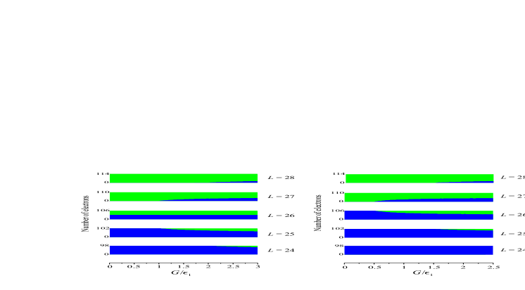
Figure 3: Filled and empty states are indicated with blue resp. green and shown as a function of the dimensionless interaction strength $G/\epsilon_{1}.$ The typical ripplon energies are smaller than the splitting between successive $L$ levels (with degeneracy $2L+1$), so that only intralevel scattering takes splace. Nevertheless the electrons are redistributed over different $L$ levels around the Fermi level $L_{F}=26$, because the pairing energy is comparable to the level splitting. The left panel shows the result for $N_{F}=52$ and the right panel for $N_{F}=106$ electrons on the Fermi level at $G=0$.

Having obtained, for the ground state, the total energy $E_{\mathrm{g.s.}}$, we can derive the condensation energy

$$E^{C}=E_{\mathrm{g.s.}}(0)-E_{\mathrm{g.s.}}(G)-G\text{ }\left\lceil N/2\right\rceil,$$ (27)

where $E_{\mathrm{g.s.}}(G)$ [$E_{\mathrm{g.s.}}(0)$] is the ground-state energy in the presence [in the absence] of the pairing interaction. The last term in the rhs describes the interaction energy for the uncorrelated Fermi ground state and $\left\lceil x\right\rceil$ means the integer part of $x$. In Fig. 4 we plot the condensation energy $E^{C}$ as a function of $G/\epsilon_{1}$. First consider the regime of strong interactions, $G\gg\epsilon_{1}/2$. For this regime, we find that the $N_{F}-$dependence of the condensation energy becomes negligible. The condensation energy rapidly rises with $G/\epsilon_{1}$, approximately as $E^{C}\approx(2L_{F}G)^{2}/(3\epsilon_{1})$. Next, consider the regime of weak interactions ($G<\epsilon_{1}/2$) where, as we have seen, the electron redistribution between the energy levels is absent. In this case the condensation energy is a linear function of $G$, and such a linear behavior can indeed be seen in Fig. 4 at $G<\epsilon_{1}/2$. In the regime of weak interaction, the condensation energy is strongly influenced by $N_{F}$: it is zero for closed shell configurations and reaches a maximum at half filling. For typical MEBs, we find that $E^{C}/k_{B}$ is of the order of several Kelvin. Decreasing the number of electrons or pressurizing the bubble increases the condensation energy. Bigger bubbles have a smaller condensation energy.

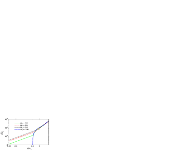
Figure 4: The condensation energy $E^{\text{C}}$ is shown as a function of the interaction strength $G$, for different numbers of electrons in the Fermi level $L_{F}=26$ at $G=0$. As the coupling increases, the condensation energy becomes less sensitive to the precise filling of the Fermi level.

III.3 Experimental signatures

How can the pairing correlations be probed experimentally ? What properties will distinguish the state with pair correlations from the normal Fermi sea ? In the preceding subsection, we have found the ground state for the system described by the Hamiltonian $H_{\text{eff}}$, expression (18), and in the preceding section we argued, based on Cooper’s argument, why this Hamiltonian is suitable to describe MEBs. Nevertheless, more exotic correlated or magnetic states not described by the Hamiltonian (18) cannot be completely excluded as candidates for the true ground state: only experiment will give a decisive answer as to what the realized state in the MEB will be. It is therefore very relevant to discuss accessible experimental signatures of the correlated many-body state that we have described.

In metallic nanograins and nanowires, pairing correlations (leading to superconductivity) were revealed through a measurement of the density of states BlackPRL76 . Also here, we propose to reveal pairing correlations by probing the density of states. In the case of stabilized MEBs SilveraBAPS , the density of states can be measured by spectroscopy. Also tunneling experiments are possible by placing an electrode close to the bubble, and reducing the thickness of the layer of helium between the bubble and the helium. The density of states that would be revealed by these experiments is the subject of the next subsection.

III.4 Density of states

In the previous subsection, we found that the ground state is characterized by a redistribution of electrons between degenerate bare energy levels, as compared to the ground-state electron distribution in the absence of interaction. Here we analyze the effect of the pairing interaction on the density of (many-electron) states in MEBs. This density of states can be written down in general as

$$\mathcal{D}(E)=\sum_{i}J^{(i)}\delta\left(E-E_{i}\right),$$ (28)

From expression (24) it is clear that the many-electron energy levels $E_{i}$ are characterized by a set of quantum numbers “$i$” $:=\{n_{L},b_{L},g_{L}\}_{L=1,2,3,...}$. The summation runs over all possible sets $i$ of quantum numbers. The degeneracy of the many-electron energy level $E_{i}$ is denoted by $J^{(i)}$. Consider one particular angular momentum state $L$ with a given {$n_{L},b_{L},g_{L}$}. The number of ways to place the unpaired electrons, multiplied by the number of pair-hole excitations with given $g_{L}$, is $J_{n_{L},g_{L},b_{L}}$ (see Refs. GladilinPRB70 ; RomanPRB67 ) :

$$J_{n_{L},g_{L},b_{L}}=2^{b_{L}}C_{b_{L}}^{2L+1}\times\left\{\begin{array}[c]{l}1,\quad g_{L}=0\\ \left(C_{g_{L}}^{2L+1-b_{L}}-C_{g_{L}-1}^{2L+1-b_{L}}\right),\quad g_{L}\geq 1\end{array}\right.$$ (29)

with $C_{j}^{k}$, the binomial coefficients. The total degeneracy is the product of the degeneracies of the independent systems,

$$J^{(i)}=\prod_{L}J_{n_{L},g_{L},b_{L}}.$$ (30)

For graphical representation, it is more convenient to consider instead of $\mathcal{D}(E)$ the quantity

$$\mathcal{D}_{\delta}(E)=\int_{E-\delta/2}^{E+\delta/2}dE\,\mathcal{D}(E),$$ (31)

which gives the number of (many-electron) states in the energy range of width $\delta$ around the energy $E$.

Fig. 5 gives an example of the calculated $\mathcal{D}_{\delta}(E)$. The calculations are performed for $N_{F}=54$ electrons in the Fermi angular momentum level $L_{F}=26$, so that in the ground state at $G=0$ the Fermi level is approximately half filled. Together with the whole spectrum of excitations (displayed in light green) we also show (in dark blue) the intralevel excitations from the ground state.

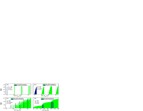
Figure 5: The calculated density of states for a spherical 2D electron system with pairing, obtained within the Richardson model, is shown in these figures as a function of the energy above the ground state energy. The different panels correspond to different strengths of the attractive electron-electron interaction term in the reduced BCS Hamiltonian.

At $G=0$, as shown in Fig. 5a, there is a set of excitations that correspond to different interlevel electron transitions between the single-electron bare energy levels with $L$ close to $L_{F}$ (obviously, intralevel transitions have zero energy in this case). At $G=0$, all the many-electron energy levels in the system under consideration are highly degenerate. This is due to the numerous possibilities to distribute electrons over single-electron states belonging to a partially filled energy level with a given $L$.

At small nonzero $G$, the many-electron energy levels for each angular momentum level are split. Excitations involving pair breaking $(b_{L}\neq 0)$ and pair-hole excitations $(g_{L}\neq 0)$ start to affect the density of states. The result, shown in Fig. 5b, is the appearance of energy bands in the density of states. The first band corresponds to intralevel excitations from the ground state, the other bands involve interlevel excitations from one angular momentum state to another.

At this point it is interesting to investigate the gap in the excitation spectrum for intralevel excitations. In superconducting nanograins, measuring such a spectroscopic gap signals the onset of superconductivity BlackPRL76 . First, consider a process where the ground state (with $n_{L}$ pairs and $b_{L}=0$ unpaired electrons) is transformed into a final state with $n_{L}^{\prime}=n_{L}-1$ and $b_{L}^{\prime}=2$ unpaired electrons. We will refer to such a process as a ‘pair-breaking excitation’. A pair-breaking ‘gap’ $\Delta^{(\text{p-b})}$ can then be defined as the energy necessary to create a pair-breaking excitation from the ground state:

$$\Delta_{L}^{(\text{p-b})}=E_{L,n_{L}-1,0,2}-E_{L,n_{L},0,0}.$$ (32)

Using (23),

$$\Delta_{L}^{(\text{p-b})}=G(2L+1).$$ (33)

Similarly, we can calculate the smallest energy needed to create a pair-hole excitation ($g_{L}=0\rightarrow g_{L}=1$) and define a pair-hole excitation gap $\Delta^{(\text{p-h})}$

$$\Delta_{L}^{(\text{p-h})} =E_{L,n_{L},1,0}-E_{L,n_{L},0,0}$$

$$=G(2L+1).$$ (34)

So, in the system under consideration, the smallest energy for a pair-breaking excitation equals that for a pair-hole excitation, $\Delta^{(\text{p-b})}=\Delta^{(\text{p-h})}$, and we can drop the superscripts (p-b) and (p-h). At $G\approx\epsilon_{1}/2$ the intralevel excitation gap $\Delta$ approaches the energy spacing $\epsilon_{1}(L+1)$ between single-electron bare energy levels with consecutive values of $L$. This means that, for $G\gg\epsilon_{1}/2$, interlevel excitations exist with energy smaller than the gap $\Delta.$ Moreover, as implied by Eq. (25), an increase of $G$ can substantially reduce the energies of interlevel transitions of pairs. At $G=0.625\epsilon_{1}$ (see Fig. 5c), the lowest interlevel excitations (green) already have energies smaller than $\Delta\$(first nonzero blue line).

At even larger $G$, pairing correlations appear on many different angular momentum levels. The pair-breaking/pair-hole excitation gap, $\Delta_{L}$, depends on the angular momentum. Therefore, as seen from Fig. 4d, the peaks of $\mathcal{D}_{\delta}(E)$ corresponding to intralevel excitations from the ground state, are split into peaks corresponding to different angular momentum states where pairing can take place. With increasing $G$, the excitation spectrum tends to become quasi-continuous, with jumps of several orders of magnitude in $\mathcal{D}_{\delta}(E)$ near the energies corresponding to pair-breaking or pair-hole excitations. Between these jumps there is a more uniform distribution of excitations, corresponding to interlevel transitions of pairs.

Fig. 6 provides an “overview” of the behavior of $\mathcal{D}_{\delta}(E)$ as a function of both $E$ and $G$ for fixed $L_{F}=26$ and two different values of $N_{F}$. One can see an interplay between intralevel excitations, whose energies always increase with increasing $G$, and excitations corresponding to interlevel transitions of pairs. For the latter, both an increase and a decrease in energy are possible with increasing $G$. While at $G\lesssim\epsilon_{1}$ the patterns of $\mathcal{D}_{\delta}(E,G)$ are very different for different $N_{F}$, at larger $G$ the behavior of $\mathcal{D}_{\delta}(E)$ in MEBs with a definite parity of the number of electrons becomes almost independent of the precise value of this number [cf. Figs. 6(a) and 6(b)]. This “universal behavior” of $\mathcal{D}_{\delta}(E)$ at large $G/\epsilon_{1}$ is further illustrated by Fig. 6, where the calculated dependence of $\mathcal{D}_{\delta}$ on $(E-E_{\mathrm{g.s.}})/\epsilon_{1}$ is shown for different $N_{F}$ and $L_{F}$. As seen from Fig. 6, neither moderate changes of $L_{F}$ nor variations of $N_{F}$ at a fixed $L_{F}$ significantly affect the shape of $\mathcal{D}_{\delta}$ versus $(E-E_{\mathrm{g.s.}})/\epsilon_{1}$ for MEBs with a given parity of the number of electrons. At the same time, Fig. 6 demonstrates a pronounced difference between the results for even MEBs and those for odd MEBs.

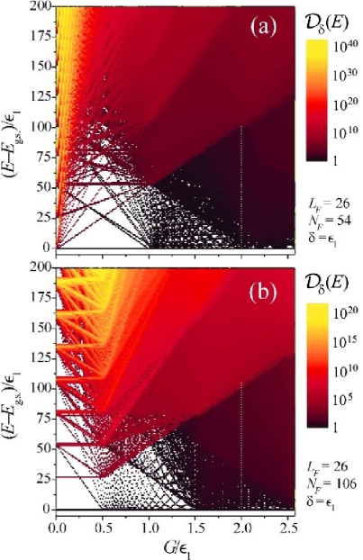
Figure 6: Density of states of the spherical 2D electron system with pairing interactions, as a function of the interaction strength and the energy above the ground state, both expressed in energy units $\epsilon_{1}$. The results are shown for two different values of $N_{F}$, the number of electrons on the Fermi level at $G=0$: (a) $N_{F}=54$ (approximately half filling) and (b) $N_{F}=106$ (closed-shell configuration).

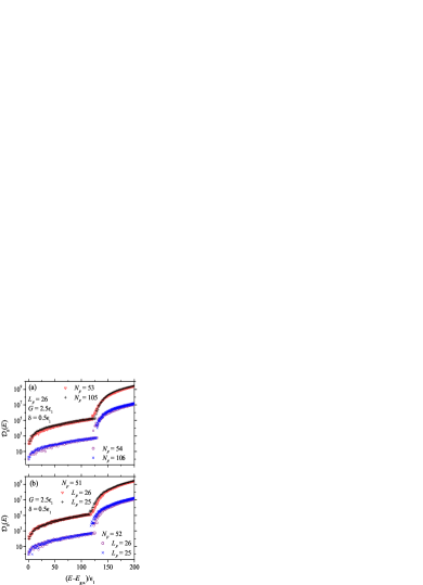
Figure 7: Density of states as a function of the energy above the ground state energy for MEBs with the pairing-interaction strength $G=2\epsilon_{1}$ and different number of electrons. Panel (a) shows the results for $L_{F}=26$ and different values of $N_{F}$, which determines the filling of the Fermi level at $G=0$. Panel (b) shows the results for two different $L_{F}$ and different parity of the number of electrons in an MEB in the case when the Fermi level is approximately half-filled at $G=0$.

Summarizing this subsection, we find that in the regime most relevant for multielectron bubbles, namely $G\gg\epsilon_{1}$, the pairing correlations reveal themselves in the density of states not as a spectroscopic gap, but rather as a significant jump in the density of states at the pair-breaking energy $\Delta$. Moreover, in this regime ($G\gg\epsilon_{1}$) the density of states is less sensitive to even-odd effects. The observation (through tunneling or spectroscopy) of a jump in the density of states at $\Delta$ can be used as a way to infer the presence of pairing correlations in the MEB. Moreover, the pair-breaking energy can be used to estimate a temperature $T_{c}$ above which the pairing correlations will be suppressed: when $k_{B}T>\Delta$ the thermal energy is large enough to support an appreciable amount of pair-breaking excitations. For typical MEBs, this temperature is of the order of Kelvins. Smaller bubbles or compressed bubbles have a larger gap and thus a larger $T_{c}$.

IV Conclusions

In the first part of this paper, we have analyzed how the electron-ripplon interaction on a spherical surface may lead to an attractive effective electron-electron interaction and give rise to a Cooper pairing scenario. The effective Hamiltonian of the two dimensional spherical electron system is mapped on a BCS-type Hamiltonian and typical values of energies, length scales and interaction strengths are estimated.

In the second part we use Richardson’s method to investigate pairing properties of a two dimensional spherical electron system. We find that when the condensation energy per pair is larger than the bubble energy scale $\hbar^{2}/(m_{e}R^{2}),$ the ground state of the system acquires unique properties that set it apart from pairing in conventional superconductors or superconducting nanograins. In particular, we show that although only intralevel interactions are included (since the relevant ripplon energies are smaller than the level splitting), electron pairs nevertheless redistribute themselves among the different levels and pairing takes place in an interval of energies around the Fermi energy, much larger than the typical ripplon energy. The density of states reveals an intricate interplay between intralevel transitions and interlevel excitation of pairs, evolving from a discrete spectrum typical for confined systems to a staircase quasi-continuum upon increasing interaction strength. At strong coupling the density of states reveal the presence of pairing correlations not through a spectroscopic gap as in metallic nanograins BlackPRL76 , but through a jump in the density of states at the pair-breaking energy.

These results show that spherical electron systems reveal particularly interesting pairing properties, distinct from their bulk or flat-surface counterparts, combining both topological effects and confinement effects. MEBs are a particularly pure realization of the two-dimensional electron system (just as an electron film on helium forms a pure realization of a flat 2DEG). Thin nanoshells (monolayer gold coatings of a non-conducting nanograin) may be another realization of this system.

- (1) Permanent address: Department of Theoretical Physics, State University of Moldova, Str. A. Mateevici 60, MD-2009 Kishinev, Republic of Moldova.
- (2) A.P. Volodin, M.S. Khaikin, and V.S. Edelman, Pis’ma Zh. Eksp. Teor. Fiz. 26, 707 (1977) [JETP Lett. 26, 543 (1977)]; U. Albrecht and P. Leiderer, Europhys. Lett. 3, 705 (1987).
- (3) R. D. Averitt, D. Sarkar, and N. J. Halas, Phys. Rev. Lett. 78, 4217 (1997); S. J. Oldenburg, R. D. Averitt, S. L. Westcott, and N. J. Halas, Chem. Phys. Lett. 288, 243 (1998); E. Prodan, P. Nordlander, and N. J. Halas, Chem. Phys. Lett. 368, 94 (2003).
- (4) J. Tempere, I. F. Silvera, and J. T. Devreese, Phys. Rev. B 65, 195418 (2002).
- (5) A. I. Goker, P. Nordlander, Journal of Physics - Condensed Matter 16, 8233 (2004).
- (6) J. Tempere, I. F. Silvera, and J.T. Devreese, Physica E: Low-dimensional Systems and Nanostructures 22, 771 (2004).
- (7) J. Tempere, I. F. Silvera and J. T. Devreese, Phys. Rev. Lett. 87, 275301 (2001).
- (8) S. N. Klimin, V. M. Fomin, J. Tempere, I. F. Silvera, J. T. Devreese, Solid State Commun. 126, 409 (2003).
- (9) M. W. Cole, Phys. Rev. B 2, 4239 (1970).
- (10) S.A. Jackson and P.M. Platzman, Phys. Rev. B 24, 499 (1981); O. Hipólito, G.A. Farias and N. Studart, Surf. Sci. 113, 394 (1982)
- (11) J. Tempere, S. N. Klimin, I. F. Silvera and J. T. Devreese, European Physical Journal B 32, 329 (2003).
- (12) L. N. Cooper, Phys. Rev. 104, 1189-1190 (1956).
- (13) R.W. Richardson, Phys. Lett. 3, 277 (1963).
- (14) F. Braun and J. von Delft, Adv. Sol. State Phys. 39, 341 (1999);
- (15) J. von Delft, A.D. Zhaikin, D.S. Golubev, and W. Tichy, Phys. Rev. Lett. 77, 3189 (1996).
- (16) K.A. Matveev and A.I. Larkin, Phys. Rev. Lett. 79, 3749 (1997).
- (17) J.M. Román, G. Sierra, and J. Dukelsky, Phys. Rev. B 67, 064510 (2003).
- (18) V.N. Gladilin, V.M. Fomin, and J.T. Devreese, Phys. Rev. B 70, 144506 (2004).
- (19) C. T. Black, D. C. Ralph, and M. Tinkham, Phys. Rev. Lett. 76, 688-691 (1996).
- (20) I. F. Silvera, J. Tempere, J. Huang, J. T. Devreese, in: Frontiers of High-Pressure Research II: Application of High Pressure to Low-Dimensional Novel Electronic Materials (eds. H. D. Hochheimer et al., Kluwer Academic Publ. 2001), p. 541-549.