Evaporative Cooling of a Guided Rubidium Atomic Beam

Abstract

We report on our recent progress in the manipulation and cooling of a magnetically guided, high flux beam of ${}^{87}{\rm Rb}$ atoms. Typically $7\times 10^{9}$ atoms per second propagate in a magnetic guide providing a transverse gradient of $800$ G/cm, with a temperature $\sim 550$ $\mu$K, at an initial velocity of 90 cm/s. The atoms are subsequently slowed down to $\sim 60$ cm/s using an upward slope. The relatively high collision rate (5 s^-1) allows us to start forced evaporative cooling of the beam, leading to a reduction of the beam temperature by a factor of 4, and a ten-fold increase of the on-axis phase-space density.

I Introduction

Evaporative cooling of atomic clouds confined in magnetic or optical traps has allowed for the realization of Bose-Einstein condensation in dilute gases bec . Coherent streams of matter waves have been extracted from such condensates, leading to the achievement of pulsed “atom lasers”laser1 ; laser2 ; laser3 ; laser4 . Nevertheless, the very low duty cycles and mean fluxes of the atom laser experiments realized to date are crucial inconveniences in view of practical applications, such as metrology or nanolithography experiments. Such applications would indeed require the equivalent, for matter waves, of a high flux, continuous-wave laser.

A possible way to realize such a cw atom laser consists in outcoupling atoms from a trap periodically replenished with new condensates ketterle . Another way to achieve this goal has been studied theoretically in mandonnet and transposes the technique of evaporative cooling to an atomic beam. A high flux, slow and cold atomic beam, transversely confined by a magnetic guide, can be further cooled by applying an energy-selective “knife” which removes atoms having a transverse energy above the average. As the remaining particles propagate further downstream and rethermalize through elastic collisions, the beam temperature decreases. By lowering the knife as the beam gets colder, forced evaporative cooling takes place, and the phase-space density of the beam increases.

The challenging prerequisite in order to apply such an evaporative cooling technique is to realize a guided atomic beam in the collisional regime, as demonstrated for the first time in PRLRb2 . Here, we report on several improvements of the setup allowing us to achieve a ten-fold increase of the beam phase-space density by evaporative cooling. An upward slope is implemented along the first 1.7 m of the guide, leading to a significant decrease of the beam velocity. This, in combination with an optimization of the pulsed injection of atoms into the guide, yields a significant increase in the collision rate. We have also developed a new detection scheme using absorption spectroscopy on an open transition, which improves the accuracy of our temperature measurements.

The article is organized as follows. In section II we describe the experimental setup, with a special emphasis on the implementation of the tilted guide which allows us to decrease the beam mean velocity. In section III we show the occurrence of non-adiabatic spin-flip losses due to the magnetic field vanishing on the guide axis. We explain how this can be circumvented by applying a longitudinal bias field. We also discuss the necessary modification of the analysis made in epjd of the temperature measurements deduced from RF spectroscopy on the atomic beam. Finally, in the last section, we report on what is, to our knowledge, the first significant gain in the phase-space density of a guided atomic beam, obtained by continuous evaporative cooling.

II Experimental setup

II.1 Magnetic guide

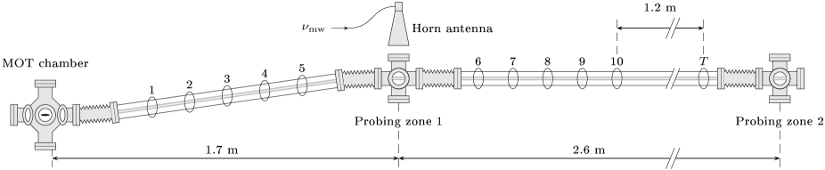
Figure 1: Simplified sketch (not to scale) of the magnetic guide. The first 1.7 m of the guide is slightly tilted upwards by $h_{0}=22\pm 1$ mm, while the remaining part is horizontal within $\pm 1$ mm. The guide sits inside glass tubes so that radio-frequency (RF) waves can be shone on the atomic beam. Two probe beams, one just after the slope, the other close to the end of the guide, can be used to detect the atoms. The beam in the Probing zone 1 can also be used as a marking beam for longitudinal time of flight measurements (see text). The ellipses numbered from 1 to 10 represent the RF antennas used for the evaporative cooling of the beam; the one labelled $T$ represents the RF antenna used to measure the beam temperature.

The magnetic guiding guide0 ; guide00 ; guide1 ; guide2 ; guide3 ; guide4 of our atomic beam is ensured by a two-dimensional quadrupole guide. The guide axis being chosen as the $z$-axis, the magnetic field reads $(bx,-by,0)$, where $b$ is the magnetic field gradient. The field increases linearly with the distance from the axis, where it vanishes, which leads to non-adiabatic spin-flip losses (see section III). Contrary to what happens with a spherical quadrupole field, this loss mechanism can be circumvented very simply by adding a longitudinal bias field $B_{0}$. The magnetic field is then non-zero everywhere. Atoms prepared in a low-field seeking state with a magnetic dipole moment $\mu$ thus experience a semi-linear cylindrically symmetric potential given by:

$$U(r)=\mu\sqrt{B_{0}^{2}+b^{2}r^{2}}\,,$$ (1)

where $r=(x^{2}+y^{2})^{1/2}$ is the radial distance from the axis. In our experiments, we use ⁸⁷Rb atoms polarized in the $|F=1,\,m_{F}=-1\rangle$ state, which has a magnetic dipole moment $\mu=\mu_{\rm B}/2$, where $\mu_{\rm B}$ is the Bohr magneton.

We denote by $\Phi$ the flux of the atomic beam propagating in the guide, $\bar{v}$ its mean velocity and $T$ its temperature. Depending on the value of the dimensionless parameter $\alpha\equiv\mu B_{0}/(k_{\rm B}T)$, the potential felt by the atoms is approximately linear (if $\alpha\ll 1$) or approximately harmonic ($\alpha\gg 1$). For arbitrary $\alpha$, exact analytical expressions for the elastic collision rate $\gamma$ within the beam, as well as for the on-axis phase space density $\rho$, can be derived for a semi-linear potential:

$$\gamma=\frac{\sigma}{2\pi^{3/2}}\,\frac{1+2\alpha}{(1+\alpha)^{2}}\,\frac{\Phi}{\bar{v}}\,\left(\frac{\mu b}{k_{\mathrm{B}}T}\right)^{2}\sqrt{\frac{k_{\mathrm{B}}T}{m}}\,,$$ (2)

$$\rho=\frac{1}{2\pi}\,\frac{1}{1+\alpha}\,\frac{\Phi}{\bar{v}}\,\left(\frac{\mu b}{k_{\mathrm{B}}T}\right)^{2}\,\frac{h^{3}}{(2\pi mk_{\mathrm{B}}T)^{3/2}}\,,$$ (3)

where $m$ is the atomic mass. In Eq. (2), the elastic collision cross-section $\sigma$ is assumed to be purely $s$-wave (and thus isotropic) and velocity-independent ($\sigma=7.6\times 10^{-16}$ m²). Both assumptions are known to be valid only if $T<100$ $\mu$K for ⁸⁷Rb. However the temperatures investigated in this article range from 150 $\mu$K to 600 $\mu$K. For those temperatures, the $d$-wave contribution has to be taken into account in the calculation of both the collision rate and the thermalization rate. The inclusion of the $d$-wave contribution in the estimation of the thermalization rate is not a straightforward task. One problem is the anisotropy of the $d$-wave differential cross-section, which reduces the efficiency of the thermalization for a given number of collisions. Another difficulty lies in interferences between $s$ and $d$-waves contributions. For the particular case of ⁸⁷Rb, the $d$-wave cross section exhibits a resonance servaas which increases the collision rate around 300 $\mu$K. This compensates partially for the reduced efficiency in rethermalization of $d$-wave scattering, resulting in a nearly constant thermalization rate dgo . Therefore, in the following, we use the expression (2) as a guideline to estimate the number of collisions.

We now turn to the experimental realization of such a guide cren . Currents up to $I=400$ A are running in four 4.5 m long parallel copper tubes sitting at the vertices of a square of side $a=8$ mm. The currents change sign between adjacent tubes. A ring-shaped, hollow, non-magnetic stainless-steel piece, brazed on the copper tubes, is used at the entrance of the guide in order to recombine the currents and the cooling water used to dissipate the $\sim 5$ kW generated by Ohmic heating. The copper tubes are held together using ceramic pieces every 30 cm, and the guide rests on other ceramic pieces which themselves rest on the inner side of the vacuum chamber. For this configuration of currents, the magnetic field gradient is $b=4\mu_{0}I/(\pi a^{2})$, and can therefore reach a maximum value of $1$ kG/cm for $I=400$ A. The magnetic field gradient is actually smaller by a factor of three at the entrance of the guide (where $a=14$ mm) and reaches its asymptotic value only after $40$ cm as the distance $a$ is progressively reduced. The goal of this tapered section is to compress adiabatically the beam during its entrance into the guide, in order to maximize the collision rate $\gamma$.

The whole guide sits in an ultra-high vacuum chamber (see Fig. 1) consisting essentially of two glass tubes allowing us to use RF antennas located outside of the vacuum chamber, since metallic tubes would screen the oscillating magnetic field. Two 25 l/s ion pumps located at $z=1.7$ m and $z=4.3$ m from the guide entrance ensure that the pressure remains around $10^{-11}$ Torr at the pumps locations; however, due to the poor conductance of the glass tubes, the effective lifetime in the second part of the guide, measured by monitoring the flux at $z=1.7$ m and $z=4.3$ m for various beam velocities, is limited to $\sim 15$ s. We find experimentally that cooling the vacuum chamber to below $-50^{\circ}$ C increases the flux measured at the end of the guide by 25% to 50%. For this purpose, we use a flow of cold nitrogen gas emanating from a liquid nitrogen dewar. This increase is a clear indication that the main source of background gas is the outgassing from the glass walls. In addition, we have found that the repeated, fast switching-off of the guide current leads to a degradation of the vacuum, presumably by causing micro-leaks to appear at the level of the brazing between the copper tubes and the recombination piece at the entrance of the guide. For this reason, we do not turn off the magnetic field of the guide when we measure the atomic beam flux, and we consequently developed a flux measurement technique (see § II.3) which is almost insensitive to the presence of the magnetic field.

II.2 Loading of the guide

In order to produce a high-flux, low velocity, cold atomic beam propagating in the guide, we use a pulsed injection scheme as described in detail in Ref. PRLRb2 . We recall here briefly the various steps involved in the 180 ms sequence used to inject a “packet” of atoms into the guide.

A slow ($\sim 20$ m/s) atomic beam, with a flux on the order of $2\times 10^{11}$ atoms/s, is produced by decelerating, in a Zeeman slower (not shown in Fig. 1), an atomic beam effusing from an oven at $140^{\circ}$ C. It is used to feed a three-dimensional magneto-optical trap (MOT). The MOT magnetic field reads $(b_{x}x,\,b_{y}y,\,b_{z}z)$ with $(b_{x},b_{y},b_{z})=(5.4,-6,0.6)$ G/cm. This anisotropy in the field gradients results in an elongated shape of the cloud. After 100 ms of loading, the MOT contains about $1.8\times 10^{9}$ atoms, and has a transverse rms radius of about $\Delta r=1$ mm and a length of 35 mm along $z$. A 3 ms launching phase occurs, in which the MOT magnetic fields are switched off, and a small frequency offset $\delta\nu$ is applied between the front and rear pairs of the MOT beams lying in the horizontal plane. In this moving molasses configuration launch , the cooling occurs in a frame moving with a velocity $v_{\rm inj}\propto\delta\nu$. This way, the atom cloud is set in motion towards the guide entrance, with an injection velocity $v_{\rm inj}$ adjustable between 30 and 250 cm/s. In the last 1.5 ms of this phase, the atoms are further cooled by increasing the laser detuning from the cooling transition to $-72$ MHz. This results in a final cloud temperature around 40 $\mu$K, hence a rms velocity $\Delta v=6$ cm/s.

A 700 $\mu$s optical pumping stage is used to pump the atoms into the $|F=1,\,m_{F}=-1\rangle$ ground state, with an efficiency of $\sim 70$%. A two-dimensional quadrupole magnetic “pre-guide” is then turned on for $80$ ms, with a transverse gradient in the $x$-$y$ plane of 85 G/cm. It prevents the atom cloud from expanding transversally and from falling due to gravity while it propagates towards the guide entrance. In order to “mode-match” the pre-guide stiffness with the cloud size and temperature, one can in principle superimpose a longitudinal bias field $B_{1}$. This makes the pre-guide harmonic, with an angular frequency $\omega_{1}\propto B_{1}^{-1/2}$. For the parameters of our atomic cloud, the field needed to obtain $\omega_{1}=\Delta v/\Delta r$ is $B_{1}=60$ G. Nevertheless, we find experimentally that applying such a bias field does not lead to appreciable changes in the beam temperature and flux. Moreover, the “center matching” (i.e., the overlapping of the atom cloud axis with the guide axis $z$), which is a crucial step in order to achieve a low temperature of the guided beam, is greatly simplified in the absence of bias field as there is no gravitational sag, whereas a bias field $B_{1}=60$ G leads to a 3 mm sag.

The atomic packets containing $1.3\times 10^{9}$ particles, and injected with a rate of (180 ms)^-1, expand longitudinally (due to the dispersion of longitudinal velocities) while they enter into the guide, and finally overlap, resulting, after a propagation over $50$ cm, in a continuous beam with a flux $\Phi=7\times 10^{9}$ atoms/s and a mean velocity $v_{\rm inj}$.

The timings cited here (100 ms of MOT loading and 80 ms of pre-guiding) are optimized for $v_{\rm inj}=90$ cm/s. For other injection velocities, these values have to be adjusted accordingly. However, it is important to point out that the pulsed injection scheme used here prevents us from injecting the beam at arbitrary low velocities. Indeed, the pre-guiding time $\tau_{\rm pg}$ must be long enough to let the packet propagate over a length $\ell$ of typically 10 cm so that the preparation of the next packet does not affect the previous one significantly. Therefore, for injection velocities much lower than 90 cm/s, the pre-guiding time $\tau_{\rm pg}\sim\ell/v_{\rm inj}$ would become prohibitively long. This would lead to a low repetition rate affecting the value of the coupled flux $\Phi$, since the number of atoms that one can accommodate in the MOT quickly saturates.

II.3 Detection of the atomic beam

Absorption spectroscopy is used to monitor the beam flux, using two laser beams located in the middle and at the end of the guide (Probing zones 1 and 2 on Fig. 1).

We have investigated two detection schemes. The first one consists in using probe beams resonant with the $|5^{2}{\rm S}_{1/2},F=2\rangle\to|5^{2}{\rm P}_{3/2},F^{\prime}=3\rangle$ transition, with a small amount of repumping light used to first repump the atoms from $|5^{2}{\rm S}_{1/2},F=1,m_{F}=-1\rangle$ to $|5^{2}{\rm S}_{1/2},F=2\rangle$. This has the advantage of yielding a continuous signal if the probe beam is locked on the transition. This allows, for example, to monitor the time dependence of the flux. The velocity measurements described in the next section are realized this way.

However, the guide magnetic field is present during those measurements. It leads to a large inhomogeneous broadening of the resonance line, largely dependent on the field gradient $b$ and on the probe beam polarization. We find that in practice, this measurement method is not reliable if one wants to measure the atomic beam flux independently of the transverse energy of the atoms. For the temperature measurements through RF spectroscopy (see below), where one is interested in such a measurement, this method can thus lead to erroneous results.

We therefore developed another technique, consisting in monitoring the absorption of the repumping beam alone. The atomic transition is obviously an open one, and the absorption is therefore quite small, on the 1% level. Nevertheless, provided the light intensity is high enough so that any atom, regardless of its position or velocity, is addressed by the laser, the number of photons absorbed per second is proportional to the atomic flux. In particular, for the transition $|5^{2}{\rm S}_{1/2},F=1\rangle\to|5^{2}{\rm P}_{3/2},F^{\prime}=2\rangle$ in which no dark state exists (in contrast to what happens for $F^{\prime}=0$ or $F^{\prime}=1$), each atom scatters on average two photons before being pumped into the $|5^{2}{\rm S}_{1/2},F=2\rangle$ level. This is therefore a convenient way to measure the absolute atomic flux in the presence of the inhomogeneous magnetic field of the guide. We find a good agreement between the flux deduced by this method and the one inferred from the loading rate of the MOT.

In practice, for measurements of relative flux, we obtain the better signal to noise ratio when we scan 70 times per second the laser frequency across the $|5^{2}{\rm S}_{1/2},F=1\rangle\to|5^{2}{\rm P}_{3/2},F^{\prime}=0,1,2\rangle$ transitions, at a rate of about $600$ MHz/ms. For a beam velocity of $\bar{v}=60$ cm/s, the atoms which are in the probing region (of length 1 mm) for a given scan were thus located $\simeq 1$ cm upstream during the previous scan and they were not affected by the probe. We find that, in contrast to the previous detection scheme, the spectra are remarkably insensitive to $b$ and to probe polarization. This robustness of the flux signal thus leads to a much more accurate temperature determination.

II.4 Implementation of a slope to slow down the beam

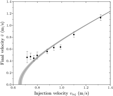
Figure 2: Velocity $\bar{v}$ of the beam after the slope as a function of the injection velocity. The magnetic gradient is $b=800$ G/cm. The solid line represents $\sqrt{v_{\rm inj}^{2}-2gh_{0}}$ with $h_{0}=22\pm 1$ mm (the shaded area represents the uncertainty in $\bar{v}$ due to the uncertainty in $h_{0}$).

Figure 3: Flux $\Phi$ measured at the end of the guide as a function of the injection velocity $v_{\rm inj}$. The magnetic guide gradient is $b=800$ G/cm. The timings of the launching sequence are kept constant with the values of Section II.2. One clearly sees that for low injection velocities, the flux decreases very significantly.

The number of collisions $N_{\rm col}$ experienced by an atom during its propagation along the whole guide scales as $1/\bar{v}^{2}$ where $\bar{v}$ is the beam mean velocity. Since the value of $N_{\rm col}$ determines the potential gain in phase-space density that one can achieve through evaporative cooling epjd , one needs to minimize $\bar{v}$. But as pointed out in § II.2, the injection velocity $v_{\rm inj}$ cannot be arbitraryly low because of the pulsed character of our loading process. Therefore, exploiting the relative mechanical flexibility of the guide and the presence of bellows in the vacuum system (see Fig. 1), we implemented an upwards slope on the first 1.7 m of the guide, the height of the guide rising by $h_{0}=22\pm 1$ mm. The remaining part of the guide is horizontal within $\pm 1$ mm (see Fig. 1). The purpose of such a slope is to decrease the mean velocity of the beam and thus increase $N_{\rm col}$. In the absence of collisions, the product of the mean velocity of the beam by the longitudinal velocity dispersion remains constant in the slope as a result of Liouville’s theorem. In a collisional beam this effect yields a slight increase of temperature by an amount $\delta T/T\sim(2/7)\delta\bar{v}/\bar{v}$ lahaye .

We have performed velocity measurements in the second part of the guide with a longitudinal time-of-flight technique. The laser beam in the Probing zone 1 on Fig. 1, located at the position $z_{1}$, is scanned at a 200 Hz rate across the transitions $|5^{2}{\rm S}_{1/2},F=1,m_{F}=-1\rangle\to|5^{2}{\rm P}_{3/2},F^{\prime},m_{F^{\prime}}\rangle$ and is used as a marking beam. For a power of 6 $\mu$W, typically 30% of the atoms are removed from the beam. At time $t=0$, we extinguish the marking beam, and we monitor with the probe located in the Probing zone 2 (locked on the cycling transition) the flux arriving at $z_{2}$. The time-dependent signal is fitted according to

$$\Phi(t)=\Phi_{0}+\Delta\Phi\,{\rm erf}\left(\frac{z_{2}-z_{1}-\bar{v}t}{t\sqrt{2k_{\mathrm{B}}T/m}}\right)\,,$$ (4)

where ${\rm erf}$ is the error function, with $T$ and $\bar{v}$ as adjustable parameters.

Fig. 2 represents the final velocity $\bar{v}$ measured this way, as a function of the injection velocity $v_{\rm inj}$. One can see a clear reduction of the velocity, with $\bar{v}$ close to the velocity $\sqrt{v_{\rm inj}^{2}-2gh_{0}}$ expected for a single particle having an initial velocity $v_{\rm inj}$ and “climbing” a height $h_{0}$ (solid line).

The use of a slope to slow down the beam is nevertheless limited by the fact that one must stay in the supersonic regime: the Mach number, defined as $\mathcal{M}=\bar{v}/\Delta v$, where $\Delta v$ is the longitudinal velocity dispersion, must remain significantly larger than $1$. If this is not true, many particles would move backwards, thereby reducing the flux (see Fig. 3) and increasing the incoming particles energy through collisions with a high relative momentum. In practice, we find that for $v_{\rm inj}=90$ cm/s, the final velocity $\bar{v}\simeq 60$ cm/s (see Fig. 2) is still high enough for the beam to stay sufficiently supersonic (for $T\sim 600$ $\mu$K, $\Delta v\sim 25$ cm/s). The net gain, induced by the use of a slope, on the number of collisions $N_{\rm col}$ is typically a factor of two for this choice of parameters.

III From linear to harmonic guiding potential

III.1 Spin-flip losses

In a purely two-dimensional quadrupole guide, the magnetic field vanishes along the guide axis $z$. Therefore, atoms having a low angular momentum experience a rapid variation of the direction of the magnetic field when they approach the axis, and can undergo a non-adiabatic spin-flip transition to an untrapped state cornell . This loss mechanism is more pronounced if the beam enters the collisional regime, since collisions redistribute angular momentum between atoms and continuously lead to new losses. Adding a longitudinal bias field to the two-dimensional quadrupole leads to a semi-linear transverse trapping potential (1), in which the magnetic field never vanishes, which can strongly suppress those Majorana losses.

Figure 4: Measured flux at the end of the guide (normalized to the flux in the absence of an applied bias field) as a function of the applied bias field $B_{\rm applied}$. The curve is not centered on $0$ because of the presence of a $B_{\rm earth}\sim 120$ mG component of the Earth magnetic field along the guide. The bias field is $B_{0}=B_{\rm applied}-B_{\rm earth}$.

To study the occurrence of such spin-flip losses in our beam, we use a solenoid wound around the guide, with a diameter varying from 30 to 50 cm and 20 turns per meter, yielding a longitudinal bias field $B_{0}=0.25$ G/A along $z$. The resulting field is uniform within $\pm 10$% along the whole guide length.

When we apply a sufficiently large bias field ($B_{0}>1$ G) the flux in the guide is enhanced by as much as 30% (see Fig. 4) with respect to its value for $B_{0}=0$. The large width of the loss curve (1 G FWHM) indicates that the observed losses are not, strictly speaking, due to Majorana spin-flips, but are probably induced by high-frequency oscillating fields (due to the noisy environment) having an amplitude of a few tenths of gauss majorana1 ; majorana2 ; majorana3 .

In practice, we operate the magnetic guide with a $B_{0}=1$ G bias field. This changes slightly the shape of the transverse trapping potential. If the beam temperature $T$ is large ($k_{\rm B}T\gg\mu B_{0}$) the trap is still approximately linear; but for lower temperatures the relevant part of the potential is harmonic.

III.2 Temperature measurements in a semi-linear potential

The exact shape of the potential needs to be taken into account in the temperature measurements that we perform with RF spectroscopy PRLRb2 . For a linear potential, we extract the beam temperature $T$ from the fraction $\varphi$ of atoms remaining in the beam after evaporation by a RF antenna operating at frequency $\nu_{\rm rf}$. If this frequency is small compared to $k_{\rm B}T/h$, then very few atoms will fulfill the RF resonance condition at some point in their trajectory and will be evaporated. In a similar way, if $h\nu_{\rm rf}\gg k_{\rm B}T$, the resonance condition is fulfilled on a radius large compared to the thermal radial size of the beam, and almost no atoms are evaporated. In between, the function $\varphi$ goes through a minimum. The same feature remains qualitatively true for a semi-linear potential, but the precise lineshape of this RF spectrum depends on the value of the bias field.

We therefore developed, for an arbitrary bias field $B_{0}$, semi-analytical calculations allowing us to extract the temperature from the curve depicting the fraction $\varphi(\nu_{\rm rf})$ of remaining atoms after the temperature measurement antenna, as a function of its RF frequency $\nu_{\rm rf}$. The method follows the one used in epjd . The curve $\varphi(\nu_{\rm rf})$ now depends on two dimensionless parameters, $\eta=h(\nu_{\rm rf}-\nu_{0})/(k_{\rm B}T)$ (where $\nu_{0}$ is the frequency corresponding to the “trap bottom”, satisfying $h\nu_{0}=\mu B_{0}$) and $\alpha=\mu B_{0}/(k_{\rm B}T)$. In the limit $\alpha\to 0$ one has a linear trap, leading to the approximate formula

$$\varphi(\eta,0)\simeq 1-1.65\,\eta^{1.13}{\rm e}^{-0.92\eta}\,,$$ (5)

while for $\alpha\to\infty$ one recovers the exact formula for a harmonic confinement:

$$\varphi(\eta,\infty)=1-\sqrt{\pi\eta}\,{\rm e}^{-\eta}\,.$$ (6)

From our calculation, we find a good interpolation between those two limits is provided by the following empirical formula:

$$\varphi_{\rm approx}(\eta,\alpha)\simeq 1-1.7\,{\rm e}^{-0.9\eta}\,\eta^{1.1-0.4\arctan(3.6\alpha)}\,.$$ (7)

We checked the validity of the approximate formula (7) by generating, with a Monte-Carlo simulation, ensembles of atoms at thermal equilibrium in the semi-linear potential, simulating the curve $\varphi(\eta,\alpha)$ by applying the evaporation criterion, and fitting this curve by Eq. (7). We find that the temperature obtained in this way is reliable within $\pm 5$% for a range of variation of $0.1\leqslant\alpha\leqslant 10$. The precision with which we can infer temperature ratios is actually better. We have checked that, for a given $B_{0}$, when two temperatures $T_{1}^{\rm sim}$ and $T_{2}^{\rm sim}$ are used to obtain simulated RF spectra, the ratio of the temperatures $T_{1}^{\rm fit}$ and $T_{2}^{\rm fit}$ obtained by fitting those spectra with Eq. (7) differs by typically less than one percent from the actual ratio $T_{1}^{\rm sim}/T_{2}^{\rm sim}$.

With this fitting function, we investigate the effect of spin-flip losses on the beam temperature. In the absence of an applied longitudinal field, we observe that the beam temperature is $\sim 8$% higher than when one applies a bias field large enough to avoid spin-flip losses. This can be easily understood since the atoms lost by spin-flips have a low angular momentum, and on average a small energy. Therefore their loss leads to a higher beam temperature after rethermalization.

IV Evaporative cooling of the beam

It is important to emphasize that applying evaporative cooling on an atomic beam is significantly more difficult than on a trapped cloud of atoms: (i) the pulsed injection results in a longitudinal dilution of the atom packets, and the resulting decrease in the atomic density yields a low initial collision rate $\gamma$, (ii) the time allowed for evaporation is limited by the guide length and by $\bar{v}$, and not only by the quality of the vacuum, and (iii) the collision rate and phase-space density scale less favorably in view of evaporative cooling for a two-dimensional confinement than for a three-dimensional trap epjd . For all those reasons, a significant gain in the phase-space density of a magnetically guided beam had never been achieved to date.

In this section, after detailing the two evaporation methods that we have developed, namely radio-frequency and microwave evaporation, we report on the evaporative cooling of the atomic beam using several evaporation zones in order to significantly increase the phase-space density.

IV.1 Radio-frequency evaporation

Evaporative cooling relying on a position-dependent transition to an untrapped state can be easily accomplished using a two-photon radio-frequency transition between the Zeeman sublevels $|F=1,m_{F}=-1\rangle$ and $|F=1,m_{F}=1\rangle$. Atoms crossing a cylinder of axis $z$, with a radius $R_{\rm evap}$ fulfilling $U(R_{\rm evap})=h\nu_{\rm rf}$, where $h$ is Planck’s constant and $\nu_{\rm rf}$ the RF frequency, are evaporated. If this radius is higher than the beam’s thermal size, essentially energetic atoms are removed, and after rethermalization, the beam gets colder. For temperatures in the range of a few hundreds $\mu$K, the corresponding frequencies are in the tens of MHz. The RF antennas that we use consist of a single loop with a 50 $\Omega$ resistor in series, in which we couple a power of $27$ dBm. This corresponds to an amplitude of the oscillating magnetic field, at the level of the atomic beam, of 50 mG.

We can measure the spatial range over which an antenna is efficient by switching on a RF antenna for a short time (a few tenths of milliseconds) and monitoring the temporal width of the dip appearing in the flux signal. We find that the typical range is around 20 cm.

Nevertheless, for some specific frequencies (especially around 40 MHz) we observe that the efficiency range of the antenna considerably increases, essentially reaching the whole guide length. Those resonance frequencies depend on the position $z_{\rm ant}$ of the antenna on the guide. This fact, added to the similarity between the guide length and the wavelengths corresponding to the resonance frequencies, leads us to suppose that the RF antennas can couple to the guide, in which they induce currents, making it act as an antenna itself.

Although those resonances are well localized in the frequency domain, and therefore do not prevent the use of RF evaporation for the purpose of evaporative cooling, we tried to circumvent this problem with evaporation in the microwave domain by inducing transitions between different hyperfine states.

IV.2 Microwave evaporation

An electromagnetic wave resonant with the hyperfine transition $|5^{2}{\rm S}_{1/2},\,F=1\rangle\to|5^{2}{\rm S}_{1/2},\,F=2\rangle$ at $\nu_{\rm hf}=6834.7$ GHz can also be used to selectively remove atoms from the beam hulet . Indeed, a magnetic dipole transition from the trapped state $|F=1,m_{F}=-1\rangle$ can only excite atoms to the anti-trapped states $|F=2,m_{F}=-2\rangle$, $|F=2,m_{F}=-1\rangle$, or to the untrapped state $|F=2,m_{F}=0\rangle$. Contrary to the RF-case, this gives three distinct evaporation radii. This leads actually to a better efficiency of the evaporative cooling process compared to single-radius evaporation, as was discussed in epjd for the case of evaporation with a continuum of radii spanning the range $[R_{\rm evap},\infty)$.

We calculate the fraction $\varphi(\nu_{\rm mw})$ of atoms remaining after such a microwave antenna operating at $\nu_{\rm mw}$, in the same way as for the single-radius evaporation scheme. Defining $\eta$ as $h(\nu_{\rm hf}-\nu_{\rm mw})/(k_{\mathrm{B}}T)$, we work out the following approximate formula, valid for a linear potential: $\varphi(\eta)=1-0.89\,\eta^{0.67}{\rm e}^{-0.27\eta}$. The shape of this curve plotted on Fig. 5 (a) is qualitatively similar to the one obtained with RF evaporation, but with a much larger width and a more pronounced minimum.

In practice, microwave evaporation is implemented by using a 10 dB gain horn antenna powered by a microwave synthesizer delivering typically 20 dBm after amplification. The directivity of such an antenna allows us to use the microwave evaporation scheme even in locations where nearby metallic walls prevent the use of RF evaporation. For instance we can use it in the metal cross located in the middle of the guide, by shining the microwave through optical viewports (see Fig. 1). We have used this evaporation scheme in order to measure the beam temperature and found a very good agreement (less than 10% difference) between microwave and RF spectroscopic measurements of temperature.

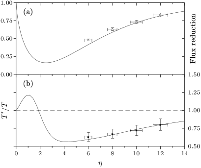
Figure 5: (a): Fraction of remaining atoms after the microwave horn antenna as a function of $\eta$. The experimental points are in good agreement with theory (solid line); the points at $\eta=6$ and 8 are slightly above the expected value, probably because of a lack of microwave power to reach a 100% efficiency in the evaporation. (b): Temperature change induced in the beam by evaporation with a microwave at the parameter $\eta$, followed by rethermalization. The solid line is the theoretical curve; the points are experimental results of evaporation performed in the interesting region where the phase-space density increases significantly. For $\eta=8$, the phase-space density of the beam increases by 2.6. For those experiments, the mean velocity is $\bar{v}=0.8$ m/s and the guide gradient $600$ G/cm.

We have also calculated the temperature change $T^{\prime}/T$ experienced by the beam upon evaporation with a microwave antenna followed by rethermalization. Fig. 5 (b) shows the corresponding theoretical curve, and the experimental data points obtained for evaporation with $\eta=6,\,8,\,10$ and 12. The beam temperature was measured with a RF antenna. The agreement is excellent, the theoretical curve having no adjustable parameters. For the point corresponding to $\eta=8$, the gain in phase-space density is $2.6$, which is significantly higher than the maximum gain of $1.9$ that one can obtain with (single-radius) RF evaporation.

IV.3 Ten-fold increase of the beam phase-space density with several antennas

In order to achieve a significant gain in phase-space density, we use the following setup (Fig. 1): We choose $v_{\rm inj}=90$ cm/s and $b=800$ G/cm. Five RF antennas, separated by $\sim 20$ cm, are placed between $0.5\leqslant z\leqslant 1.3$ m with frequencies decreasing from $49$ to 25 MHz, then the horn antenna at $z=1.7$ m is operated at $\nu_{\rm mw}=6774$ MHz, and finally five more RF antennas are placed at $2\leqslant z\leqslant 2.8$ m with frequencies decreasing from $21$ to $14$ MHz. We use such a scheme, in which obviously no complete rethermalization can occur between successive RF antennas, because it is less sensitive to a potential lack of efficiency of an antenna for some frequency. In addition, this scheme is closer to the usual evaporation ramp in the time domain used for evaporative cooling of trapped atoms than the step-like evaporation process that would consist in letting the beam rethermalize completely after each antenna.

The last evaporation antenna being placed at $z=2.8$ m, and the analysis antenna used for the temperature measurements at $z=4$ m, the beam can rethermalize completely after the last antenna, and therefore we measure the temperature of a beam which is really in thermal equilibrium.

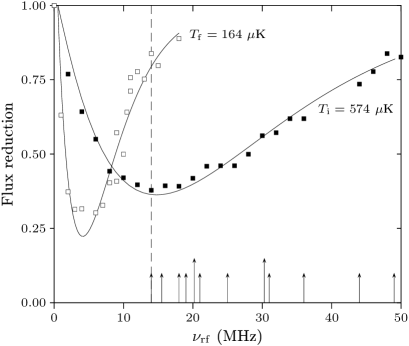
Figure 6: Radio-frequency spectra used to determine the temperature of the atomic beam with and without evaporation by 10 RF antennas and the horn antenna. The temperature reduction from 574 to 164 $\mu$K, accompanied by a flux reduction by a factor 7.7, leads to a ten-fold increase of the phase-space density. The arrows represent the evaporation frequencies of the 10 RF antennas. The two longer arrows correspond to RF frequencies that would lead to the existence of evaporation radii coinciding with the ones resulting from microwave evaporation by the horn; another one at 60.7 MHz is not shown on the figure.

Fig. 6 shows the RF spectra from which we deduce the initial (without evaporation) and final (after evaporation by the 10 RF and microwave antennas) temperatures $T_{\rm i}$ and $T_{\rm f}$. We find $T_{\rm i}=574\pm 9$ $\mu$K, and $T_{\rm f}=164\pm 6$ $\mu$K. The corresponding flux reduction is $\Phi_{\rm f}/\Phi_{\rm i}=0.13\pm 0.02$. From this we infer a gain in phase-space density by a factor $10.4^{+4.1}_{-3.0}$. The spectrum giving $T_{\rm f}$ corresponds to a well thermalized beam (the spectrum does not reach the value 1 for, e.g., $\nu_{\rm rf}=14$ MHz, which would be the signature PRLRb2 of the absence of rethermalization after the last evaporation antenna). This configuration corresponds to the existence of a steady-state temperature gradient $dT/dz\simeq 200$ $\mu$K/m along the beam.

Those measurements require a good stability of the incident atomic flux. Indeed, a small relative variation $\delta\Phi_{\rm i}/\Phi_{\rm i}$ can be amplified very significantly since a decrease in $\Phi_{\rm{}_{i}}$ will result in less collisions between successive antennas, and thus in a more pronounced reduction of the flux than in the collisional case. We observed that fluctuations in $\Phi_{\rm i}$ by 30% could lead to fluctuations above 50% in $\Phi_{\rm f}$. For the data of Fig. 6 we therefore checked that the absolute flux was almost constant and equal to its maximal value during the whole data acquisition.

V Conclusion and prospects

In this article, we have demonstrated the first significant gain in the phase-space density of a magnetically guided atomic beam by means of continuous evaporative cooling. This ten-fold increase brings the beam’s phase-space density to about $2\times 10^{-7}$. In order to gain the seven remaining orders of magnitude required to reach quantum degeneracy, the temperature needs to be decreased so much that the guide confinement will become harmonic. As pointed out in epjd , the evaporation becomes less efficient for this confinement as compared to the linear case, and the elastic collision rate cannot increase significantly during the evaporation process.

In order to have a quantitative picture of the whole evaporation ramp all the way to quantum degeneracy, we therefore calculated for arbitrary values of $\alpha$, the change in flux and temperature for a given value of $\eta$. This allows one to calculate, through Eq. (2) and (3), the gain in phase-space density and the evolution of the collision rate.

The resulting “evaporation trajectories” followed by the beam in the plane $(T,\,\Phi)$ when it crosses successive single-radius evaporation antennas are plotted on Fig. 7 and 8. The frequency of each antenna is adapted so as to evaporate at constant $\eta$ parameter, and we assume that full rethermalization occurs after each antenna. One sees that evaporating at relatively low $\eta$ minimizes the number of antennas needed to reach degeneracy, but implies to have very low final flux and temperatures, in the 30 nK range. Simultaneously, the collision rate for such low evaporation parameters is decreasing significantly in the final evaporation stages when the temperature is low and the potential harmonic (see Fig. 8). On the contrary, evaporating at too large $\eta$ requires too many antennas and thus a very long guide.

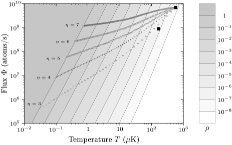
Figure 7: Theoretical “trajectories” to quantum degeneracy followed by the beam in the plane $(T,\,\Phi)$ during evaporation with many antennas, at constant $\eta$. The grey scale represents the on-axis phase-space density $\rho$ (which scales as $\Phi/T^{7/2}$ in the linear regime $\alpha\ll 1$, and as $\Phi/T^{5/2}$ in the harmonic regime). The atomic beam propagates with a velocity of $60$ cm/s in a magnetic guide having a transverse gradient of 800 G/cm, with a longitudinal bias field of 1 G. The initial flux is $7\times 10^{9}$ atoms/s, and the initial temperature 570 $\mu$K. Each symbol in the various evaporation trajectories corresponds to the action of one antenna. For higher evaporation parameters $\eta$, the final flux and temperatures (when $\rho=1$) are higher, but this requires more antennas (the number of antennas required to reach $\rho=1$ for $\eta=3$, 4, 5, 6 and 7, is 41, 64, 106, 181, and 306, respectively). The black squares represent the experimental beam parameters before and after evaporation with the method described in § IV.3.

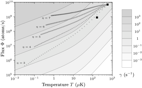
Figure 8: Same as Fig 7, but with a grey scale representing the elastic collision rate $\gamma$, assuming that the collision cross section is purely s-wave, and constant in magnitude (both assumptions fail above typically 100 $\mu$K). The cross-over from a linear trap (in which $\gamma\sim\Phi/T^{3/2}$) to a harmonic trap (where $\gamma\sim\Phi/T^{1/2}$) is clearly visible when $k_{\rm B}T$ becomes on the order of $\mu B_{0}$ (here, at $T\sim 30$ $\mu$K since $B_{0}=1$ G). Runaway evaporation, ie constant increase of $\gamma$, can only occur for large values of $\eta$; for $\eta=4$, which requires a moderate number of antennas, $\gamma$ starts by increasing at the beginning of the evaporation, when the trap is still linear, but then decreases as the guide becomes more and more harmonic.

A promising strategy probably consists in operating the antennas with $\eta=4$ or 5, requiring a number of antennas between 60 and 100. Nonetheless, due to the finite range of the antennas, with such a large number of evaporation zones one probably needs to abandon the simple model of discrete evaporation zones followed by rethermalization mewes , and resort to a continuous evaporation model as the one used in standard BEC experiments and considered in mandonnet . The atomic energy distribution is then at any time close to a truncated Boltzmann distribution walraven , whereas we considered here that enough time was allowed between two successive antennas to recover an exact equilibrium. Another possibility would consist in using surface evaporation cornellJLTP by approaching solid surfaces close to the beam, on which the most energetic atoms would stick: this would allow for the use of many very localized evaporation zones.

- (1) Unité de Recherche de l’Ecole Normale Supérieure et de l’Université Pierre et Marie Curie, associée au CNRS.
- (2) C. J. Pethick and H. Smith, Bose-Einstein Condensation in Dilute Gases, (Cambridge University Press, Cambridge, 2002); L. P. Pitaevskii and S. Stringari, Bose-Einstein condensation, (Clarendon Press, Oxford, 2003).
- (3) M.-O. Mewes, M. R. Andrews, D. M. Kurn, D. S. Durfee, C. G. Townsend, and W. Ketterle, Phys. Rev. Lett. 78, 582 (1997).
- (4) I. Bloch, T. W. Hänsch and T. Esslinger, Phys. Rev. Lett. 82, 3008 (1999).
- (5) E. W. Hagley, L. Deng, M. Kozuma, J. Wen, K. Helmerson, S. L. Rolston, and W. D. Phillips, Science 283, 1706 (1999).
- (6) Y. Le Coq, J. H. Thywissen, S. A. Rangwala, F. Gerbier, S. Richard, G. Delannoy, P. Bouyer, and A. Aspect, Phys. Rev. Lett. 87, 170403 (2001).
- (7) A. P. Chikkatur, Y. Shin, A. E. Leanhardt, D. Kielpinski, E. Tsikata, T. L. Gustavson, D. E. Pritchard, and W. Ketterle, Science 296, 2193 (2002).
- (8) E. Mandonnet, A. Minguzzi, R. Dum, I. Carusotto, Y. Castin and J. Dalibard, Eur. Phys J. D 10, 9 (2000).
- (9) T. Lahaye, J. M. Vogels, K. Guenter, Z. Wang, J. Dalibard, and D. Guéry-Odelin, Phys. Rev. Lett. 93, 093003 (2004).
- (10) T. Lahaye and D. Guéry-Odelin, Eur. Phys. J. D 33, 67 (2005).
- (11) J. Schmiedmayer, Phys. Rev. A 52, R13-R16 (1995).
- (12) A. Goepfert, F. Lison, R. Schütze, R. Wynands, D. Haubrich, and D. Meschede, Appl. Phys. B 69, 217 (1999).
- (13) M. Key, I. G. Hughes, W. Rooijakkers, B. E. Sauer, E. A. Hinds, D. J. Richardson, and P. G. Kazansky, Phys. Rev. Lett. 84, 1371 (2000).
- (14) N. H. Dekker, C. S. Lee, V. Lorent, J. H. Thywissen, S. P. Smith, M. Drndic, R. M. Westervelt, and M. Prentiss, Phys. Rev. Lett. 84, 1124 (2000).
- (15) B. K. Teo and G. Raithel, Phys. Rev. A 63, 031402 (2001).
- (16) J. A. Sauer, M. D. Barrett, and M. S. Chapman, Phys. Rev. Lett. 87, 270401 (2001).
- (17) S. J. J. M. F. Kokkelmans, B. J. Verhaar, K. Gibble, and D. J. Heinzen, Phys. Rev. A 56, R4389 (1997).
- (18) M. Anderlini and D. Guéry-Odelin, in preparation.
- (19) P. Cren, C. F. Roos, A. Aclan, J. Dalibard, and D. Guéry-Odelin, Eur. Phys J. D 20, 107 (2002).
- (20) A. Clairon, C. Salomon, S. Guellati and W.D. Phillips, Europhys. Lett., 16, 165 (1991).
- (21) T. Lahaye, P. Cren, C. Roos, and D. Guéry-Odelin, Comm. Nonlin. Sci. Num. Sim. 8, 315 (2003).
- (22) W. Petrich, M. H. Anderson, J. R. Ensher, and E. A. Cornell, Phys. Rev. Lett. 74, 3352 (1995).
- (23) C. V. Sukumar and D. M. Brink, Phys. Rev. A 56, 2451 (1997).
- (24) S. Gov, S. Shtrikman and H. Thomas, J. Appl. Phys. 87, 3989 (1999).
- (25) E. A. Hinds and C. Eberlein, Phys. Rev. A 61, 033614 (2000).
- (26) C. C. Bradley, C. A. Sackett, J. J. Tollett, and R. G. Hulet, Phys. Rev. Lett. 75, 1687 (1995).
- (27) K. B. Davis, M.-O. Mewes, and W. Ketterle, Appl. Phys. B 60, 155 (1995).
- (28) O. J. Luiten, M. W. Reynolds, and J. T. M. Walraven, Phys. Rev. A 53, 381 (1996).
- (29) D. M. Harber, J. M. McGuirk, J. M. Obrecht, and E. A. Cornell, J. Low Temp. Phys. 133, 229 (2003).