Tunnel junction as a noise probe

Abstract

The paper investigates theoretically effects of noise on low-bias parts of $IV$ curves of tunnel junctions. The analysis starts from the effect of shot noise from an additional (noise) junction on the Coulomb blockaded Josephson junction in high-impedance environment. Asymmetry of shot noise characterized by its odd moments results in asymmetry of the $IV$ curve of the Josephson junction. At high currents through the noise junction the $IV$ curve is very sensitive to electron counting statistics. The theory is generalized on another type of noise (phase noise of a monochromatic AC input), on a normal Coulomb blockaded tunnel junction. The effect of shot noise on the $IV$ curve of a superconducting Josephson junction in low-impedance environment is also analyzed. From this effect one can obtain information on the time necessary for an electron to tunnel through the junction responsible for shot noise. In summary, the analysis demonstrates, that the low-bias part of the $IV$ curves of tunnel junctions can be a sensitive probe of various types of noise.

I Introduction

The problem of noise and decoherence plays the important role both for applications and for fundamental physics. Noise parameters for electron transport provide a valuable information, which is not available from average current-voltage dependences. This stimulates development of effective methods of noise investigation. In particular, a lot of attention is devoted to shot noise Blanter , which is related to discreteness of charge transport and yields direct information on carrier charges. Efforts of theorists were invested to studying full counting statistics of shot noise, its non-Gaussian character Lez and asymmetry (odd moments) Odd ; BKN . They are also objects of intensive experimental investigations Reul ; Rez .

Recently it was shown that the zero-bias anomaly of the incoherent Cooper-pairs current in a Coulomb blockaded Josephson junction is very sensitive to shot noise from an independent source and therefore can be used for noise investigation SN . Further experimental and theoretical investigations exp ; SN-T ; Heik have demonstrated that this method especially useful for studying asymmetry of shot noise, which is connected with its non-Gaussian character and is very difficult for detection by other methods of noise spectroscopy Reul ; Rez . In addition, other methods to use the Josephson junction as a noise probe were discussed. Deblock et al. Delft suggested to use the quasiparticle current for noise detection. The scheme to use the Josephson junction as a threshold detector of electron counting statistics has also been investigated theoretically and experimentally TN ; Pek ; Grab . The scheme exploited the effect of noise on macroscopical quantum tunneling at currents close to the critical current.

The goal of this paper is to extend the theoretical analysis of the effect of noise on the low-bias part of the $IV$ curve of a mesoscopic tunnel junction. The previous analysis SN ; exp ; SN-T addressed the effect of shot noise on a Coulomb blockaded Josephson junction in the weak-coupling limit, when the Josephson coupling energy $E_{J}$ was small compared to the Coulomb energy $E_{c}=e^{2}/C$. Here $C$ is the relevant capacitance. Shot noise originated from a low current through a parallel junction, and its effect on the $IV$ curve of the Josephson junction had asymmetry connected with the non-Gaussian character of shot noise. The effect was insensitive to counting statistics of the noise current since the latter was so low that the single-electron tunneling events were well separated in time and their correlation was not essential. On the basis of the fulfilled analysis one could expect that a Coulomb blockade normal junction is also able to effectively probe noise, and other types of noise different from shot noise can be investigated, but in order to check these expectations an additional analysis was needed. The present paper is to give answers to the following questions:

• Can the zero-bias anomaly of the probing junction be sensitive to the counting statistics of electrons tunneling through the noise source (noise junction) when the current through the noise junction grows?

• Is the zero-bias anomaly of the Coulomb blockaded normal tunnel junction also sensitive to noise similarly to the Coulomb blockaded Josephson junction?

• Is the zero-bias anomaly of the Coulomb blockaded tunnel junction sensitive to other types of noise different from shot noise?

• Can the Josephson junction in the strong coupling limit $E_{J}\gg E_{C}$ also probe noise?

The paper gives positive answers to all these questions. The content of the paper is the following. Section II reminds the previous analysis SN ; exp ; SN-T for the Coulomb blockade Josephson junction in the weak coupling limit $E_{J}\ll E_{c}$ and extends it on the case of higher noise currents, when the zero-bias anomaly is expected to be sensitive to the electron counting statistics. The analysis confirms this expectation. At high currents the effect is essentially different for the cases of strictly periodical sequence of pulses and of random pulses governed by the Poissonian statistics. Section III considers another type of noise: phase fluctuations in a monochromatic microwave signal, which result in decoherence of the signal. A similar phase noise is well known in quantum optics. It is shown that the effect of the microwave on the $IV$ curve of the Josephson junction gives direct information on the decoherence time. Section IV addresses the effect of shot noise on the zero-bias anomaly of a normal tunnel junction. The latter is also very sensitive to shot noise and phase fluctuations in an AC input, and therefore can be exploited as a noise detector. Section V considers the Josephson junction in the strong coupling limit in low-impedance environment. This case was chosen because it allows to exploit its duality to the case of the Josephson junction in the weak coupling limit in high-impedance environment, which was considered in the previous sections. But duality is valid mostly for the equilibrium Nyquist-Johnson noise. For shot noise duality does not work, and the effect of noise on the Josephson junction in low impedance environment (superconductive regime) is different from that in high impedance environment (Coulomb blockade regime). The important feature of the low-impedance case is the perspective to measure the intrinsic tunneling time, which is discussed in the end of Sec. V.

II Josephson junction, weak coupling limit, shot noise

II.1 Without shot noise

Let us review well known results concerning the $IV$ curve without shot noise. We assume that the Josephson coupling energy $E_{J}\cos\varphi$ ($\varphi$ is the Cooper-pair phase difference between two banks of the Josephson junction) is weak in comparison with the Coulomb energy $E_{c}=e^{2}/2C$, where $C$ is the relevant capacitance (see below), and the Josephson coupling can be considered as a time-dependent perturbation. Then the Golden Rule gives for the current of Cooper pairs Aver ; SZ ; IN :

$$I={\pi eE_{J}^{2}\over\hbar}[P(2eV)-P(-2eV)]~{},$$ (1)

where the function

$$P(E)={1\over 2\pi\hbar}\int_{0}^{\infty}dt\,\left[e^{iEt/\hbar}\left\langle e^{i\varphi(t_{0})}e^{-i\varphi(t_{0}-t)}\right\rangle+e^{-iEt/\hbar}\left\langle e^{i\varphi(t_{0}-t)}e^{-i\varphi(t_{0})}\right\rangle\right]$$ (2)

characterizes the probability to transfer the energy $E>0$ to environment (or to absorb the energy $|E|$ from environment if $E<0$) at the time $t_{0}$. In many cases (equilibrium and shot noise included) the average phase correlators do not depend on the time $t_{0}$ after averaging, and Eq. (2) is reduced to the Fourier component of the average phase correlator IN :

$$P(E)={1\over 2\pi\hbar}\int_{-\infty}^{\infty}dt\,e^{iEt/\hbar}\left\langle e^{i\varphi(t)}e^{-i\varphi(0)}\right\rangle~{}.$$ (3)

However studying the linear response to the AC input in Sec. III.1 we shall need the more general expression Eq. (2).

Since we use the perturbation theory with respect to $E_{J}$ we can calculate phase fluctuations neglecting $E_{J}$, i.e., treating the Josephson junction as a capacitor. The crucial assumption in the phase-fluctuation theory (or $P(E)$ theory) is that the phase fluctuations are Gaussian IN and

$$\langle e^{i\varphi_{0}(t_{0})}e^{-i\varphi_{0}(t_{0}-t)}\rangle\approx e^{J_{0}(t)}~{},$$ (4)

where the phase–phase correlator

$$J_{0}(t)=\langle[\varphi_{0}(t)-\varphi_{0}(0)]\varphi_{0}(0)\rangle=J_{R}(t)+iJ_{I}(t)=2\int_{-\infty}^{\infty}{d\omega\over\omega}\frac{\mbox{Re}Z(\omega)}{R_{Q}}\frac{e^{-i\omega t}-1}{1-e^{-\beta\hbar\omega}}$$ (5)

is a complex function of time. The subscript 0 points out that the phase fluctuation $\varphi_{0}$ is determined by the equilibrium Johnson-Nyquist noise in the environment, i.e., in the electric circuit with the impedance $Z(\omega)$. Here $R_{Q}=h/4e^{2}=\pi\hbar/2e^{2}$ is the quantum resistance for Cooper pairs and $\beta=1/k_{B}T$ is the inverse temperature. Then IN

$$P(E)={1\over\pi\hbar}\mbox{Re}\left\{\int_{0}^{\infty}dt\exp\left[J_{0}(t)+\frac{iEt}{\hbar}\right]\right\}\,,$$ (6)

and the current is

$$I=-{2eE_{J}^{2}\over\hbar^{2}}\mbox{Im}\left\{\int_{0}^{\infty}dte^{J_{0}(t)}\sin\left(2eVt\over\hbar\right)\right\}~{}.$$ (7)

The zero-bias conductance is given by

$$G_{0}=\left.{dI\over dV}\right|_{V\rightarrow 0}=-{4e^{2}E_{J}^{2}\over\hbar^{3}}\mbox{Im}\left\{\int_{0}^{\infty}t\,dte^{J_{0}(t)}\right\}\,.$$ (8)

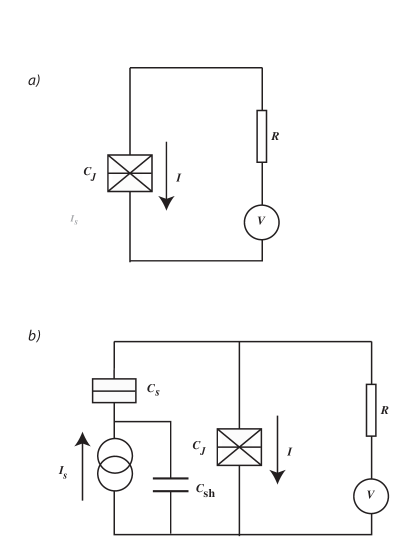
Figure 1: Electric circuit. a) The Josephson junction voltage-biased through the shunt resistance $R$. b) Parallel to the Josephson junction the normal junction with the capacitance $C_{s}$ is switched on, which produces shot noise affecting the current through the Josephson junction. The large shunt capacitance $C_{sh}$ transforms at finite frequencies the current bias into the voltage bias.

The electric circuit for our analysis is shown in Fig. 1a. The Josephson tunnel junction with capacitance $C_{J}$ is voltage-biased via the shunt resistor $R$. Thus in our case $Z(\omega)=(1/R+i\omega C)^{-1}$ with $C=C_{J}$, and

$$J_{0}(t)=2\rho\int_{-\infty}^{\infty}{d\omega\over\omega}\frac{1}{1+\omega^{2}\tau^{2}}\frac{e^{-i\omega t}-1}{1-e^{-\beta\hbar\omega}}~{},$$ (9)

where $\tau=RC$ and $\rho=R/R_{Q}$. At $T\to 0$ ($t>0$):

$$J_{0}(t)=\rho\left[-e^{t/\tau}\mbox{E}_{1}\left({t\over\tau}\right)-e^{-t/\tau}\mbox{E}_{1}\left(-{t\over\tau}+i0\right)-2\ln{t\over\tau}-2\gamma-i\pi\right]\,,$$ (10)

where $\gamma=0.577$ is the Euler constant, and $\mbox{E}_{1}(z)=\int_{1}^{\infty}(e^{-zt}/t)\,dt$ is the exponential integral AS . The small imaginary correction $+i0$ to the argument of one of the exponential integrals is important for analytic continuation of $\mbox{E}_{1}(z)$ from real $t$ to the complex plane AS (see below). At $T=0$ $P(E)$ vanishes for $E<0$ since it is the probability of the transfer of the energy $|E|$ from the environment to the junction, which is impossible if $T=0$.

For further analysis we need the expressions for $J_{0}$ in the limits of short time $t\ll\tau$:

$$J_{0}(t)\approx\rho\left[{t^{2}\over\tau^{2}}\left(\ln{t\over\tau}+\gamma-{3\over 2}\right)-{i\pi t\over\tau}\right]\,,$$ (11)

and long time $t\gg\tau$:

$$J_{0}(t)=-\rho\left(2\ln{t\over\tau}+2\gamma+i\pi\right)\,.$$ (12)

The function $P(E)$, as well as the current $I$, which it determines, have been carefully studied and calculated for arbitrary $\rho$ Ing . But for the goals of our analysis it is useful to present a simplified calculation valid only in the high impedance limit $\rho\gg 1$. In this limit integration in the expression for the conductance $G_{0}$, Eq. (8), should be done over rapidly oscillating functions and it is difficult to see that the integral exactly vanishes at $T=0$. But it becomes evident after rotation of the integration path in the plane of complex time, which corresponds to replacing $t$ by $-iy$. This rotation transforms the integration over the positive real semiaxis into the integration over the negative imaginary semiaxis. After this transformation, the complex function $J_{0}(t)\to J_{0}(-iy)$ becomes a purely real function, and the conductance $G_{0}$, which is given by the imaginary part of this function, vanishes. This is true for any term $V^{k}$ in the expansion of the current $I$ in voltage $V$ as far as the integral over $t$, which determines this term, converges at long time. Using the asymptotic expression Eq. (12) one can see that the integral is divergent if $k>2\rho-2$. So at zero temperature the current $I$ as a function of $V$ does not vanish completely but is given by a small nonanalytic power-law term, which can be found in the limit of high $\rho$ from the following simple steepest descent estimation of the integral.

Expecting that the main contribution comes from long times one can rewrite the expression (6) for the $P(E)$ function using the asymptotic expression (12) for $J_{0}$:

$$P(E)={1\over\pi\hbar}\mbox{Re}\left\{\int_{0}^{\infty}dt\,\exp\left[-\rho\left(2\ln{t\over\tau}+2\gamma+i\pi\right)+{iEt\over\hbar}\right]\right\}~{}.$$ (13)

The saddle point is determined by the condition of vanishing first derivative of the argument of the exponential function: $-{2\rho/t_{0}}+{iE/\hbar}=0$. This yields $t_{0}=-2i\hbar/E$. Expanding the argument of the exponential function around the saddle point ($t^{\prime}=t-t_{0}$) we receive

$$P(E)={1\over\pi\hbar}\mbox{Re}\left\{\exp\left[\rho\left(-2\gamma-2\ln{2\rho\hbar\over iE\tau}-i\pi\right)+2\rho\right]\right\}\int_{-\infty}^{\infty}dt^{\prime}\,\exp\left(-{E^{2}\over 4\rho\hbar^{2}}t^{\prime 2}\right)$$

$$=\exp[2\rho(1-\gamma)]{\tau\over\sqrt{\pi\rho}\hbar}\left(E\tau\over 2\rho\hbar\right)^{2\rho-1}~{}.$$ (14)

Finally

$$I={\pi eE_{J}^{2}\over\hbar}P(2eV)=\sqrt{\pi\over{\rho}}\exp[2\rho(1-\gamma)]{eE_{J}^{2}\tau\over\hbar^{2}}\left(eV\tau\over\rho\hbar\right)^{2\rho-1}~{}.$$ (15)

In summary, if environment provides only the equilibrium noise, the low-bias part of the $IV$ curve is governed by phase correlations at very long time, which yield in the limit $\rho\gg 1$ an extremely small nonanalytic current.

II.2 With shot noise

Now we consider the effect of shot noise from an independent source. Parallel to the Josephson junction there is another junction (noise junction) with the capacitance $C_{s}$ connected with an independent DC current source (see Fig. 1b). The resistance of the noise junction is very large compared to the shunt resistance $R$. The role of very large capacitance $C_{sh}$ is to shortcircuit the large ohmic resistance of the current source for finite frequencies. The current $I_{s}$ through the noise junction produces shot noise, which affects the $IV$ curve of the Josephson junction.

In the presence of shot noise the fluctuating phase $\varphi=\varphi_{0}+\varphi_{s}$ consists of two terms: $\varphi_{0}$ from Johnson-Nyquist noise, and $\varphi_{s}$ from shot noise. For calculation of the shot-noise fluctuations $\varphi_{s}$ we assume that the charge transport through the noise junction is a sequence of current peaks $\delta I=\mbox{sign}(I_{s})e\sum_{i}\delta(t-t_{i})$, where $t_{i}$ are random moments of time when an electron crosses the junction Blanter . We neglect duration of the tunneling event itself. The positive sign of $I_{s}$ corresponds to the current shown in Fig. 1b. Any peak generates a voltage pulse at the Josephson junction: $V_{s}(t)=\mbox{sign}(I_{s})(e/C)\sum_{i}\Theta(t-t_{i})e^{-(t-t_{i})/\tau}$, where $\Theta(t)$ is the step function and $C=C_{J}+C_{s}$. The voltage pulses result in phase jumps determined by the Josephson relation $\hbar\partial\varphi_{s}/\partial t=2eV_{s}$. The sequences of current and voltage peaks and phase jumps are shown in Fig. 2.

Calculating the contribution from shot noise fluctuations $\varphi_{s}$ to the phase correlators one should abandon the assumption that noise is Gaussian [Eq. (4)]. On the other hand, we assume that the phase fluctuation $\varphi_{s}$ is classical and the values of $\varphi_{s}$ at different moments of time commute. Since equilibrium noise and shot noise are uncorrelated, the generalization of Eq. (7) is

$$I=-{2eE_{J}^{2}\over\hbar^{2}}\mbox{Im}\left\{\int_{0}^{\infty}dte^{J_{0}(t)}\left\langle\sin\left({2eVt\over\hbar}+\Delta\varphi_{s}\right)\right\rangle\right\}.$$ (16)

The phase difference between two moments $t_{0}$ and $t_{0}-t$, $\Delta\varphi_{s}=\varphi_{s}(t_{0})-\varphi_{s}(t_{0}-t)=\sum_{i}\delta\varphi_{s}(t,t_{0}-t_{i})$, is a sum of contributions from random current peaks, each of them determined by

$$\delta\varphi_{s}(t,\tilde{t})=\mbox{sign}(I_{s})\pi\rho\left\{\Theta(\tilde{t})\left[1-e^{-(\tilde{t})/\tau}\right]-\Theta(\tilde{t}-t)\left[1-e^{-(\tilde{t}-t)/\tau}\right]\right\}~{},$$ (17)

where $\tilde{t}=t_{0}-t_{i}$. Since phase jumps are not small for $\rho\gg 1$, one cannot use the perturbation theory with respect to them. The interpretation of the expression Eq. (16) for the current is straightforward: As far as the random phase difference $\Delta\varphi_{s}=2e\int^{t_{0}}_{t_{0}-t}V_{s}(t^{\prime})dt^{\prime}/\hbar$ is classical, it should be simply added to the phase difference $\varphi_{V}=2eVt/\hbar$ generated by the constant voltage bias $V$.

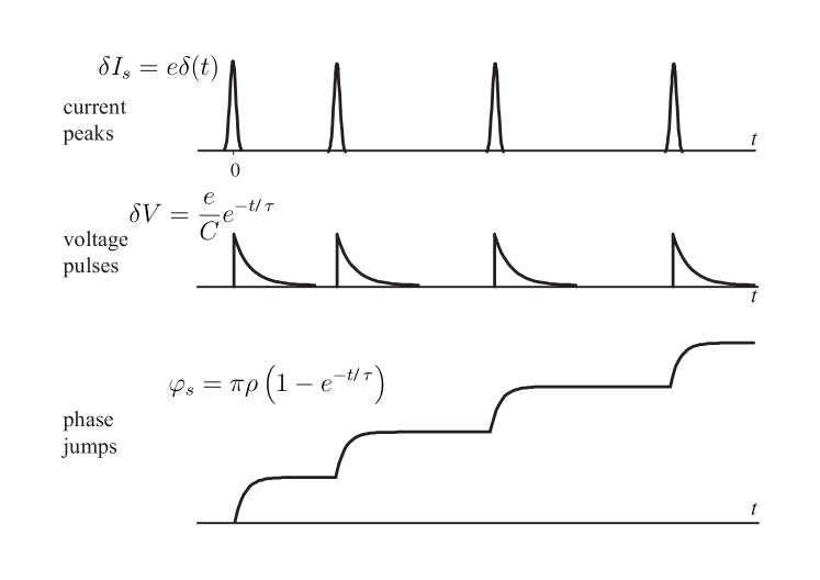
Figure 2: Current and voltage pulses, phase jumps.

Let us consider the case of the Poissonian statistics. If one performs observation during a very long period of time $\tau_{\infty}$, the number of pulses during this period is large and close to $N\sim|I_{s}|\tau_{\infty}/e$. Keeping in mind the absence of correlation between pulses, the phase correlator after averaging over the long time $\tau_{\infty}$ is

$$\left\langle e^{i\Delta\varphi_{s}}\right\rangle=\left\langle e^{i\sum_{j}\delta\varphi_{s}(t,t_{0}-t_{j})}\right\rangle=\left\langle e^{i\delta\varphi_{s}}\right\rangle^{N}\approx\left(1+{\Phi(t)\over\tau_{\infty}}\right)^{N}~{},$$ (18)

where $\Phi(t)=\Phi_{c}(t)+i\Phi_{s}(t)$ is determined by the integrals over a single phase jump (corresponding to a single current pulse):

$$\Phi_{s}(t)=\int_{-\infty}^{\infty}d\tilde{t}\sin\delta\varphi_{s}(t,\tilde{t})=\tau{I_{s}\over|I_{s}|}\left\{{\pi\over 2}+\mbox{si}\left[r\left(1-e^{-t/\tau}\right)\right]+\sin r\left[\mbox{ci}r-\mbox{ci}\left(re^{-t/\tau}\right)\right]-\cos r\left[\mbox{si}r-\mbox{si}\left(re^{-t/\tau}\right)\right]\right\}$$ (19)

and

$$\Phi_{c}(t)=\int_{-\infty}^{\infty}d\tilde{t}\left[\cos\delta\varphi_{s}(t,\tilde{t})-1\right]=\tau\left\{\mbox{ci}\left[r\left(1-e^{-t/\tau}\right)\right]+\cos r\left[\mbox{ci}r-\mbox{ci}\left(re^{-t/\tau}\right)\right]\right.$$

$$\left.+\sin r\left[\mbox{si}r-\mbox{si}\left(re^{-t/\tau}\right)\right]-\gamma-\ln\left[r\left(1-e^{-t/\tau}\right)\right]\right\}-t~{}.$$ (20)

Here $\mbox{si}(x)=-\int_{x}^{\infty}\sin t\,dt/t$ and $\mbox{ci}(x)=-\int_{x}^{\infty}\cos t\,dt/t$ are sine and cosine integral functions AS , and $r=\pi\rho$. In the limit $\tau_{\infty}\to\infty$ and $N\to\infty$ at $N/\tau_{\infty}=|I_{s}|/e$ the phase correlator is

$$\left\langle e^{i\Delta\varphi_{s}}\right\rangle=\exp\left[{N\Phi(t)\over\tau_{\infty}}\right]=\exp\left[{|I_{s}|\over e}\Phi(t)\right]~{}.$$ (21)

Finally the expression for the current, Eq. (16), can be written as

$$I=-{2eE_{J}^{2}\over\hbar^{2}}\mbox{Im}\left\{\int_{0}^{\infty}dte^{J_{0}(t)}\exp\left({|I_{s}|\over e}\Phi_{c}\right)\sin\left({2eVt\over\hbar}+{|I_{s}|\over e}\Phi_{s}\right)\right\}.$$ (22)

In contrast to the case without shot noise, when the expansion of the current $I$ in a small voltage bias starts from the nonanalytic term $\propto V^{2\rho-1}$, in the presence of shot noise the expansion in $V$ starts with analytic terms:

$$I=I_{0}+G_{s}V+aV^{2}+bV^{3}~{},$$ (23)

where

$$G_{s}=-{4e^{2}E_{J}^{2}\over\hbar^{3}}\int_{0}^{\infty}t\,dt\mbox{Im}\left\{e^{J_{0}(t)}\right\}[\left\langle\cos\Delta\varphi_{s}\right\rangle-1]$$ (24)

is the shot-noise conductance,

$$I_{0}=-{2eE_{J}^{2}\over\hbar^{2}}\int_{0}^{\infty}dt\mbox{Im}\left\{e^{J_{0}(t)}\right\}\left\langle\sin\Delta\varphi_{s}\right\rangle$$ (25)

is the ratchet current, and the parameters

$$a={4e^{3}E_{J}^{2}\over\hbar^{4}}\int_{0}^{\infty}t^{2}\,dt\mbox{Im}\left\{e^{J_{0}(t)}\right\}\left\langle\sin\Delta\varphi_{s}\right\rangle$$ (26)

and

$$b={8e^{4}E_{J}^{2}\over 3\hbar^{5}}\int_{0}^{\infty}t^{3}\,dt\mbox{Im}\left\{e^{J_{0}(t)}\right\}[\left\langle\cos\Delta\varphi_{s}\right\rangle-1]$$ (27)

determine the curvature of the conductance-voltage plot and the shift of the conductance minimum. Without shot noise all these integrals vanish at $\rho\gg 1$ [see the paragraph after Eq. (12)].

In Refs. exp, ; SN-T, the parameters of the analytic expansion of $I(V)$ were calculated for low currents $|I_{s}|\ll e/\tau$ through the noise junction, when voltage pulses and phase jumps are well separated in time (see Fig. 2). Then the relevant phase correlators are proportional to the density $|I_{s}|/e$ of pulses in time SN-T :

$$\langle e^{i\Delta\varphi_{s}}\rangle-1=\langle\cos\Delta\varphi_{s}\rangle-1+i\langle\sin\Delta\varphi_{s}\rangle={|I_{s}|\over e}\Phi(t)={|I_{s}|\over e}[\Phi_{c}(t)+i\Phi_{s}(t)]~{}.$$ (28)

The parameters determined by $\left\langle\cos\Delta\varphi_{s}\right\rangle$ correspond to “even” effects (the conductance is symmetric with respect to voltage inversion $V\to-V$), which are present also without shot noise. Therefore the contribution from shot noise to these parameters should be added to the values derived from Gaussian equilibrium noise. In contrast, the parameters determined by $\left\langle\sin\Delta\varphi_{s}\right\rangle$ correspond to “odd” (asymmetric) effects, which are absent for equilibrium noise and are related to the non-Gaussian character of shot noise.

In the high-impedance limit $\rho\gg 1$ it is possible to calculate the parameters of the $IV$ curve analytically. As one can see below, the most important contributions to the integrals, which determine $G_{s}$, $a$, and $b$, come from times $t\sim\tau/\sqrt{\rho\ln\rho}$ short compared to $\tau$, and one may use the small-argument expansion for the Johnson-Nyquist correlator given in Eq. (11). On the other hand, these times are long enough for using asymptotic expansions for the sine and the cosine integrals: $\mbox{si}(x)\sim-\cos x/x-\sin x/x^{2}$, $\mbox{ci}(x)\sim\sin x/x-\cos x/x^{2}$. Then one can rewrite Eq. (19) as

$$\Phi_{s}(t)\approx\tau\left\{{\pi\over 2}+{1\over r}-{\cos\left[r\left(1-e^{-t/\tau}\right)\right]\over re^{-t/\tau}}-{\cos\left[r\left(1-e^{-t/\tau}\right)\right]\over r(1-e^{-t/\tau})}\right.$$

$$\left.+{\sin\left[r\left(1-e^{-t/\tau}\right)\right]\over r^{2}e^{-2t/\tau}}-{\sin\left[r\left(1-e^{-t/\tau}\right)\right]\over r^{2}(1-e^{-t/\tau})^{2}}\right\}\approx\tau\left[{\pi\over 2}-{\tau\over rt}\cos{rt\over\tau}-{\tau^{2}\over r^{2}t^{2}}\sin{rt\over\tau}\right]~{}.$$ (29)

In Eq. (20) it is enough to keep only the main asymptotic terms $\propto 1/r$:

$$\Phi_{c}(t)\approx\tau\left\{-{t\over\tau}+{\sin\left[r\left(1-e^{-t/\tau}\right)\right]\over re^{-t/\tau}}+{\sin\left[r\left(1-e^{-t/\tau}\right)\right]\over r(1-e^{-t/\tau})}-\gamma-\ln\left[r\left(1-e^{-t/\tau}\right)\right]\right\}$$

$$\approx\tau\left[-{t\over\tau}-\ln{rt\over\tau}-\gamma+{\tau\over rt}\sin{rt\over\tau}\right]~{}.$$ (30)

Let us consider first the parameters connected with “even” effects. For low currents $|I_{s}|\ll e/\tau$:

$$G_{s}\approx-{4eE_{J}^{2}\tau\over\hbar^{3}}|I_{s}|\int_{0}^{\infty}t\,dt\mbox{Im}\left\{e^{J_{0}(t)}\right\}{\tau\over rt}\sin{rt\over\tau}$$

$$\approx{4eE_{J}^{2}\tau^{2}\over\hbar^{3}r}|I_{s}|\int_{0}^{\infty}dt\exp\left(-\rho{t^{2}\over\tau^{2}}\ln{\tau\over t}\right)\sin^{2}{rt\over\tau}\approx{\sqrt{2}\pi eE_{J}^{2}\tau^{3}\over\hbar^{3}r^{3/2}\sqrt{\ln r}}|I_{s}|\approx{\pi^{5/2}E_{J}^{2}C^{3}\over 4e^{5}\sqrt{2\ln\rho}}\rho^{3/2}|I_{s}|~{},$$ (31)

$$b={8e^{3}E_{J}^{2}\tau\over 3\hbar^{5}}|I_{s}|\int_{0}^{\infty}t^{3}\,dt\mbox{Im}\left\{e^{J_{0}(t)}\right\}{\tau\over rt}\sin{rt\over\tau}$$

$$\approx-{8e^{3}E_{J}^{2}\tau^{2}\over 3\hbar^{5}r}|I_{s}|\int_{0}^{\infty}t^{2}\,dt\exp\left(-\rho{t^{2}\over\tau^{2}}\ln{\tau\over t}\right)\sin^{2}{rt\over\tau}\approx-{2\pi^{2}\sqrt{2}e^{3}E_{J}^{2}\tau^{5}\over 3\hbar^{5}r^{5/2}(\ln r)^{3/2}}|I_{s}|\approx-{\pi^{2}C^{2}\rho\over 6e^{2}\ln\rho}G_{s}~{}.$$ (32)

The main contributions to these integrals come from the last term in the asymptotic expansion Eq. (30). The other terms either vanish (term $\propto\gamma$) or are of higher orders (terms $\propto t$ and $\propto\ln t$) with respect to $1/r$. A negative sign of $b$ means that in the center of the zero-bias anomaly the curve “conductance vs. voltage” has a maximum but not a minimum. However this is possible to see only at very low temperatures since finite temperatures give a positive contribution to the curvature parameter $b$.

In a similar way one can calculate the asymmetry integral

$$a=-{4e^{2}E_{J}^{2}\tau\over\hbar^{4}}I_{s}\int_{0}^{\infty}t^{2}\,dt\mbox{Im}\left\{e^{J_{0}(t)}\right\}{\tau^{2}\over r^{2}t^{2}}\sin{rt\over\tau}={I_{s}\over|I_{s}|}{C\over 2e}G_{s}~{}.$$ (33)

Here the main contribution comes from the last term of the asymptotic expansion Eq. (29).

For the integral in Eq. (25), which determines the ratchet current $I_{0}$, the relevant times are shorter than for the other integrals: $t\sim\tau/\rho\sim R_{Q}C$. Therefore one cannot use the asymptotic expansion Eq. (29). Instead one can integrate by parts, and for low noise currents:

$$I_{0}=-{2eE_{J}^{2}\over\hbar^{2}}{|I_{s}|\over e}\int_{0}^{\infty}dt\mbox{Im}\left\{e^{J_{0}(t)}\right\}\Phi_{s}(t)\approx{2E_{J}^{2}\over\hbar^{2}}|I_{s}|\int_{0}^{\infty}dt\Phi_{s}(t)\sin{rt\over\tau}={2E_{J}^{2}\tau\over\hbar^{2}r}|I_{s}|\int_{0}^{\infty}dt\frac{d\Phi_{s}(t)}{dt}\cos{rt\over\tau}$$

$$\approx{2E_{J}^{2}\tau^{2}\over\hbar^{2}r}I_{s}\int_{0}^{\infty}{dt\over t}\cos{rt\over\tau}\sin{rt\over\tau}={\pi E_{J}^{2}\tau^{2}\over 2\hbar^{2}r}I_{s}={\pi^{2}E_{J}^{2}C^{2}\over 8e^{4}}\rho I_{s}\,.$$ (34)

II.3 Shot noise from high currents and electron counting statistics

Shot noise is non-Gaussian and asymmetric, but in the case of low noise currents its effect does not depend on statistics of electron transport and is determined only by density of current pulses in time. Even if pulses were not random and formed a strictly periodical sequence the effect would be the same. In order to obtain information on counting statistics from measurements of the $IV$ curve the noise current should be not small compared with the width of the voltage pulse $\sim\tau$. One could expect SN-T that in the limit of high noise current $I_{s}$ discreteness of the electron transport through the junction would be less and less essential and eventually the effect of the current $I_{s}$ would be reduced to the constant voltage drop $V_{s}=I_{s}R$ on the shunt resistor $R$ resulting in a trivial shift of the voltage applied to the Josephson junction. If it were the case, the long-time asymptote for the phase correlator would be

$$\langle e^{i\Delta\varphi_{s}}\rangle\to\exp\left(2ieV_{s}t\over\hbar\right)=\exp\left(2ieI_{s}Rt\over\hbar\right)=\exp\left(ir{I_{s}t\over e}\right)~{}.$$ (35)

This asymptotic behavior really takes place for a strictly periodic sequence of current pulses with period $T_{0}=e/|I_{s}|$. In this case the phase variation for the time interval $nT_{0}<t<(n+1)T_{0}$ ($n$ is integer) is:

$$\varphi(t)=r\left[n+{1-e^{-(t-nT_{0})/\tau}\over 1-e^{-T_{0}/\tau}}\right]~{}.$$ (36)

In the limit $|I_{s}|\to\infty$ ($T_{0}\to 0$) the maximum deviation of the phase from the linear function $\varphi(t)=rt/T_{0}$ is of the order $rT_{0}^{2}/\tau^{2}$, i.e., vanishes in this limit. This yields Eq. (35).

However, the expression (21) derived from the Poissonian statistics has another asymptotic behavior for $t\to\infty$:

$$\langle e^{i\Delta\varphi_{s}}\rangle-1\to\exp\left[\left(e^{ir}-1\right){I_{s}t\over e}\right]~{}.$$ (37)

Thus the $IV$ curve of the Josephson junction essentially depends on whether the current pulses through the parallel (noise) junction are strictly periodical in time, or completely random. This proves strong sensitivity to counting statistics.

Note that the right-hand side of Eq. (37) coincides with the characteristic function $\chi(r)=\sum_{n}P_{n}e^{irn}$ for the Poissonian distribution $P_{n}=e^{-\bar{n}}\sum_{n}\bar{n}^{n}/n!$ with $\bar{n}=I_{s}t/e$. This is a natural result since the number of phase jumps $n=\Delta\varphi_{s}/2\pi$ during a long time $t\gg\tau$ coincides with the number of electrons transmitted through the noise junction during the same time interval. Equation (37) leads to a conclusion that in the case of the Poissonian statistics shot noise affects the $IV$ curve even at high noise currents when one might expect suppression of noise effects. This suppression takes place for usual methods of noise detection probing voltage fluctuations. Indeed calculating the voltage variance $\langle\Delta V^{2}\rangle$ for the Poissonian statistics,

$$\langle\Delta V^{2}\rangle=\langle V^{2}\rangle-\langle V\rangle^{2}={e\over 2C}\langle V\rangle~{},$$ (38)

one obtains that the relative mean-square-root voltage fluctuation $\sqrt{\langle\Delta V^{2}\rangle}/\langle V\rangle$ vanishes at $V_{s}=\langle V\rangle=I_{s}R\to\infty$. However, the Coulomb blockaded junction probes not voltage but phase, which is much more sensitive to fluctuations. This “supersensitivity” of the Coulomb blockaded junction to fluctuations explains why the effects of higher moments (or cummulants) are much stronger than in usual methods of noise detection BKN ; Reul ; Rez .

III Josephson junction, weak coupling limit, phase noise in the AC input

Now we want to demonstrate that the Coulomb blockaded junction can effectively probe not only shot noise but other types of noise as well. As an example, phase fluctuations in a monochromatic electromagnetic wave will be considered. This type of noise is very important for lasers L , but the present analysis addresses microwaves. Suppose that some microwave source provides an input signal described by phase variation at the Josephson junction:

$$\varphi_{i}=\varphi_{0}\sin\psi(t)=\varphi_{0}\sin\left[\omega t+\sum_{i}\gamma_{i}\Theta(t-t_{i})\right]~{},$$ (39)

where $\gamma_{i}$ are random phase jumps at random moments of time $t_{i}$. Frequency of phase jumps is characterized by the average time $\tau_{c}$ between the jumps. In fact $\tau_{c}$ is nothing else as the decoherence time of the microwave signal. We shall see that the $IV$ curve of the Josephson junction is very sensitive to the decoherence process. But in order to demonstrate it one should first consider the response of the Josephson junction to a strictly monochromatic noiseless microwave input.

III.1 Response to a monochromatic AC input

For a strictly monochromatic signal the phase difference between the moments $t_{0}$ and $t_{0}-t$ is

$$\Delta\varphi_{i}(t_{0},t)=\varphi_{i}(t_{0})-\varphi_{i}(t_{0}-t)=\varphi_{0}[\sin\omega t_{0}-\sin\omega(t_{0}-t)]=\varphi_{0}[\sin\omega t_{0}(1-\cos\omega t)+\cos\omega t_{0}\sin\omega t]~{}.$$ (40)

In full analogy with the previous cases, the current is given by

$$I=-{2eE_{J}^{2}\over\hbar^{2}}\mbox{Im}\left\{\int_{0}^{\infty}dte^{J_{0}(t)}\sin\Delta\varphi_{i}(t_{0},t)\right\}~{},$$ (41)

but now averaging over the moment $t_{0}$ is not done. The linearization with respect to the input gives

$$I\approx-{2eE_{J}^{2}\over\hbar^{2}}\mbox{Im}\left\{\int_{0}^{\infty}dte^{J_{0}(t)}\Delta\varphi_{i}(t_{0},t)\right\}=-\varphi_{0}{2eE_{J}^{2}\over\hbar^{2}}\mbox{Im}\left\{\int_{0}^{\infty}dte^{J_{0}(t)}[\cos\omega t_{0}\sin\omega t+\sin\omega t_{0}(1-\cos\omega t)]\right\}$$

$$=I_{1}\cos\omega t_{0}+I_{2}\sin\omega t_{0}~{}.$$ (42)

Thus the tunneling current of Cooper pairs consists of two parts: one is out of phase and another is in phase with the input voltage $V_{i}=V_{0}\cos\omega t$ (the reactive and the active responses) where $V_{0}=\hbar\omega\varphi_{0}/2e$. Comparing the active response,

$$I_{1}=-\varphi_{0}{2eE_{J}^{2}\over\hbar^{2}}\mbox{Im}\left\{\int_{0}^{\infty}dte^{J_{0}(t)}\sin\omega t\right\}~{},$$ (43)

with Eq. (7) one can see that the ohmic current as a function of frequency can be directly received from the $IV$ curve $I(V)$ replacing voltage $V$ by $\hbar\omega/2e$. Therefore the active (ohmic) response is given by

$$I_{1}=\varphi_{0}I\left(\hbar\omega\over 2e\right)=V_{0}{2e\over\hbar\omega}I\left(\hbar\omega\over 2e\right)~{}.$$ (44)

Thus the ohmic AC linear conductance of the junction is a nonanalytic function of frequency proportional to $\omega^{2\rho-2}$.

The reactive response for frequencies $\omega\ll\rho/\tau=1/R_{Q}C$ is

$$I_{2}=-\varphi_{0}{2eE_{J}^{2}\over\hbar^{2}}\mbox{Im}\left\{\int_{0}^{\infty}dte^{J_{0}(t)}(1-\cos\omega t)\right\}\approx-\varphi_{0}{eE_{J}^{2}\over\hbar^{2}}\mbox{Im}\left\{\int_{0}^{\infty}dte^{J_{0}(t)}\omega^{2}t^{2}\right\}~{}.$$ (45)

After rotation in the complex plane ($t\to-iy$):

$$I_{2}=-\varphi_{0}{eE_{J}^{2}\over\hbar^{2}}\omega^{2}\int_{0}^{\infty}y^{2}dye^{-\pi\rho y/\tau}=-\varphi_{0}{2eE_{J}^{2}\over\hbar^{2}}\omega^{2}\left(\tau\over\pi\rho\right)^{3}=-V_{0}{2e\over\hbar\omega}{2eE_{J}^{2}\over\hbar^{2}}\omega^{2}\left(R_{Q}C\over\pi\right)^{3}=-V_{0}\omega C{E_{J}^{2}C^{2}\over 2e^{4}}~{}.$$ (46)

The linear dependence on frequency points out that this current corresponds to the capacitance element of the electrical circuit. Indeed, the effective circuit for the Josephson junction has the capacitance $C$ in parallel to the tunneling conductance element. But in the presence of the Josephson coupling the geometric capacitance should be replaced by the effective capacitance (like the mass of an electron in a periodic potential should be replaced by the effective mass, see, e.g., Ref. SZ, ). The current component $I_{2}$ is related with the difference between the effective and the geometric capacitance in the weak coupling limit. In order to check it one should calculate the second-order (with respect to the Josephson coupling) correction to the Coulomb energy $Q^{2}/2C$:

$$E={Q^{2}\over 2C}+\sum_{Q_{G}\neq 0}{V(Q_{G})^{2}\over E_{0}(Q)-E_{0}(Q+Q_{G})}~{},$$ (47)

where summation is over the inverse-lattice “wave-numbers” (charges) $Q_{G}=2en$ ($n$ is any integer). For weak Josephson coupling only two terms $Q_{G}=\pm 2e$ of the sum are important, and $V(\pm 2e)=E_{J}/2$. Then

$$E={Q^{2}\over 2C}+{E_{J}^{2}\over 4}\left[{2C\over Q^{2}-(Q+2e)^{2}}+{2C\over Q^{2}-(Q-2e)^{2}}\right]={Q^{2}\over 2C}+{E_{J}^{2}\over 4}{e^{2}C\over e^{4}-e^{2}Q^{2}}\approx{Q^{2}\over 2C}+{E_{J}^{2}C\over 4e^{2}}-{E_{J}^{2}C\over 4e^{4}}Q^{2}~{}.$$ (48)

This yields for the effective capacitance:

$${1\over C^{*}}={d^{2}E\over dQ^{2}}={1\over C}-{E_{J}^{2}C\over 2e^{4}}~{},$$ (49)

and it is evident that the reactive component $I_{2}$ of the tunneling current is determined by $\Delta C=C^{*}-C$. It is useful to rewrite the expression for this correction using the Ambegoakar-Baratoff relation:

$$E_{J}={\pi\hbar\Delta\over 4e^{2}R_{T}}={\Delta_{0}\over 2}{R_{Q}\over R_{T}}~{},$$ (50)

where $\Delta_{0}$ is the bulk superconducting gap. Then the capacitance correction is

$$\Delta C=C{E_{J}^{2}C^{2}\over 2e^{4}}=C{R_{Q}^{2}\over R_{T}^{2}}{\Delta_{0}^{2}\over 8e^{4}/C^{2}}~{}.$$ (51)

Now we calculate the nonlinear (quadratic) effect of the AC input on the DC conductance. This requires averaging (over the period of the AC input) of the quadratic term in the expression for the conductance:

$$\Delta G=-{4e^{2}E_{J}^{2}\over\hbar^{3}}\mbox{Im}\left\{\int_{0}^{\infty}t\,dte^{J_{0}(t)}\langle\cos\Delta\varphi_{i}\rangle\right\}\approx{2e^{2}E_{J}^{2}\over\hbar^{3}}\mbox{Im}\left\{\int_{0}^{\infty}t\,dte^{J_{0}(t)}\langle\Delta\varphi_{i}^{2}\rangle\right\}$$

$$=\varphi_{0}^{2}{2e^{2}E_{J}^{2}\over\hbar^{3}}\mbox{Im}\left\{\int_{0}^{\infty}t\,dte^{J_{0}(t)}(1-\cos\omega t)\right\}~{}.$$ (52)

The expansion in $\omega$ contains only the terms even in $t$. The integrals over these terms vanish after rotation in the plane of complex time. This means that $\Delta G$ is determined by a very small nonanalytic contribution from long times FBS . The presence of noise essentially changes the situation as we shall see in the next subsection.

III.2 Phase noise

In the presence of the phase noise, when the phase varies according to Eq. (39), the squared difference between the phases at the moments of time $t_{0}$ and $t_{0}-t$ averaged over the time $t_{0}$ is given by

$$\langle\Delta\varphi_{i}(t_{0},t)^{2}\rangle=\varphi_{0}^{2}\langle[\sin\psi(t_{0})-\sin\psi(t_{0}-t)]\rangle^{2}=\varphi_{0}^{2}\{1-\langle\cos[\psi(t_{0})-\psi(t_{0}-t)]\rangle\}\,.$$ (53)

The average $\langle\cos[\psi(t_{0})-\psi(t_{0}-t)]\rangle$ does not vanish only if there is no random phase jumps in the time interval $t$. Assuming the Poisson distribution the probability of the absence of random phase jumps in the interval $t$ is $e^{-t/\tau_{c}}$, where $\tau_{c}$ is the average period between random phase jumps. Then one obtains that

$$\langle\Delta\varphi_{i}(t_{0},t)^{2}\rangle=\varphi_{0}^{2}(1-\cos\omega te^{-t/\tau_{c}})~{}.$$ (54)

Finally the correction to the DC conductance [compare with Eq. (52)] is:

$$\Delta G=\varphi_{0}^{2}{2e^{2}E_{J}^{2}\over\hbar^{3}}\mbox{Im}\left\{\int_{0}^{\infty}t\,dte^{J_{0}(t)}(1-\cos\omega te^{-t/\tau_{c}})\right\}\approx\varphi_{0}^{2}{2e^{2}E_{J}^{2}\over\hbar^{3}\tau_{c}}\mbox{Im}\left\{\int_{0}^{\infty}t^{2}\,dte^{J_{0}(t)}\right\}~{}.$$ (55)

After rotation in the complex plane the imaginary part of the integral does not vanish, and

$$\Delta G=\varphi_{0}^{2}{2e^{2}E_{J}^{2}\over\hbar^{3}\tau_{c}}\int_{0}^{\infty}y^{2}\,dye^{-\pi\rho y/\tau}=\varphi_{0}^{2}{4e^{2}E_{J}^{2}\tau^{3}\over\pi^{3}\rho^{3}\hbar^{3}\tau_{c}}=\varphi_{0}^{2}{E_{J}^{2}C^{3}\over 2e^{4}\tau_{c}}=V_{0}^{2}{2E_{J}^{2}C^{3}\over e^{2}\hbar^{2}\omega^{2}\tau_{c}}~{}.$$ (56)

This contribution to the zero-bias conductance essentially exceeds the small nonanalytic contribution from the strictly monochromatic microwave and provides direct information on the decoherence time $\tau_{c}$.

IV Normal junction, shot noise

IV.1 The $IV$ curve in the time-domain formulation (without shot noise)

This subsection reminds the $P(E)$ theory for a normal Coulomb blockaded junction IN . The current is given by

$$I={e}[\Gamma^{+}(V)-\Gamma^{-}(V)]~{},$$ (57)

where the forward tunneling probability is

$$\Gamma^{+}(V)={1\over e^{2}R_{T}}\int_{-\infty}^{\infty}dE\frac{E}{1-\exp\left(-\frac{E}{T}\right)}P(eV-E)~{}.$$ (58)

Here $P(E)$ is given by Eq. (6). The backward tunneling rate is $\Gamma^{-}(V)=\Gamma^{+}(-V)$. Since now we consider tunneling of single electrons (instead of Cooper pairs) the correlation function is given by

$$J_{0}(t)=\langle[\varphi(t)-\varphi(0)]\varphi(0)\rangle=2\int_{-\infty}^{\infty}{d\omega\over\omega}\frac{\mbox{Re}Z(\omega)}{R_{K}}\frac{e^{-i\omega t}-1}{1-e^{-\beta\hbar\omega}}~{},$$ (59)

where the single electron quantum resistance $R_{K}=h/e^{2}$ replaces the Cooper-pair quantum resistance $R_{Q}=h/2e^{2}$ in Eq. (5). In the case of purely ohmic environment, $Z(\omega)=R/(1+i\tau\omega)$, one can use the time-domain formulation JED fulfilling integration over energy $E$ in Eq. (58):

$$\Gamma^{+}(V)={1\over\pi\hbar e^{2}R_{T}}\mbox{Re}\left\{\int_{0}^{\infty}dt\gamma(t)\exp\left[J_{0}(t)+\frac{ieVt}{\hbar}\right]\right\}~{}.$$ (60)

Here $\tau=RC$ as before, and

$$\gamma(t)=\int_{-\infty}^{\infty}dE\frac{E}{1-\exp\left(-\frac{E}{T}\right)}\exp\left(-\frac{iEt}{\hbar}\right)=i\pi\hbar^{2}{d\over dt}\delta(t)-{\pi^{2}\over\beta^{2}}\frac{1}{\sinh^{2}(\pi t/\hbar\beta)}~{}.$$ (61)

Then after some simple algebra the current is

$$I={e}[\Gamma^{+}(V)-\Gamma^{-}(V)]={1\over R_{T}}\left[V+{2\pi\over e\hbar\beta^{2}}\mbox{Im}\left\{\int_{0}^{\infty}\frac{dt}{\sinh^{2}(\pi t/\hbar\beta)}e^{J_{0}(t)}\sin\frac{eVt}{\hbar}\right\}\right]~{}.$$ (62)

At $T=0$:

$$I={1\over R_{T}}\left[V+{2\hbar\over\pi e}\mbox{Im}\left\{\int_{0}^{\infty}\frac{dt}{t^{2}}e^{J_{0}(t)}\sin\frac{eVt}{\hbar}\right\}\right]~{},$$ (63)

and the differential conductance is

$$G={dI\over dV}={1\over R_{T}}\left[1+{2\over\pi}\mbox{Im}\left\{\int_{0}^{\infty}\frac{dt}{t}e^{J_{0}(t)}\cos\frac{eVt}{\hbar}\right\}\right]~{}.$$ (64)

For $\rho=R/R_{K}\gg 1$ in the limit $V\to 0$ the conductance vanishes:

$$G_{0}={1\over R_{T}}\left[1-{2\over\pi}\int_{0}^{\infty}\frac{dt}{t}\sin\left(\pi\rho{t\over\tau}\right)\right]\to 0~{},$$ (65)

but there remains a small nonanalytic contribution, which originates from long times: $G_{0}\propto V^{2\rho}$.

IV.2 Effect of shot noise

Repeating derivation of the effect of the random phase from shot noise, which was done above for the Josephson junction, one receives that the effect on the normal tunnel junction is similar: the linear phase from the constant voltage, $eVt/\hbar$, must be replaced by the phase $eVt/\hbar+\Delta\varphi_{s}$, where $\Delta\varphi_{s}=\varphi_{s}(t_{0})-\varphi_{s}(t_{0}-t)$ is the phase difference produced by the current through the noise junction. Note that the Josephson relation between the voltage and the phase from shot noise is different from that for the Josephson junction by the factor of 2: $V_{s}(t)=(\hbar/e)d\varphi_{s}(t)/dt_{s}$. Then the probability of the forward tunneling is [instead of Eq. (60)]

$$\Gamma^{+}(V)={1\over\pi\hbar e^{2}R_{T}}\mbox{Re}\left\{\int_{0}^{\infty}dt\gamma(t)\left\langle\exp\left(J(t)+\frac{ieVt}{\hbar}+i\Delta\varphi_{s}\right)\right\rangle\right\}~{},$$ (66)

and the total current is

$$I={e}[\Gamma^{+}(V)-\Gamma^{-}(V)]={1\over R_{T}}\left[V+V_{s}+{2\pi\over e\hbar\beta^{2}}\mbox{Im}\left\{\int_{0}^{\infty}\frac{dt}{\sinh^{2}(\pi t/\hbar\beta)}e^{J(t)}\left\langle\sin\left(\frac{eVt}{\hbar}+\Delta\varphi_{s}\right)\right\rangle\right\}\right]~{}.$$ (67)

Here $V_{s}=I_{s}R$ is the average voltage generated by the current through the noise junction. In the $T=0$ limit the current is:

$$I={1\over R_{T}}\left[V+V_{s}+{2\hbar\over\pi e}\mbox{Im}\left\{\int_{0}^{\infty}\frac{dt}{t^{2}}e^{J(t)}\left\langle\sin\left(\frac{eVt}{\hbar}+\Delta\varphi_{s}\right)\right\rangle\right\}\right]~{}.$$ (68)

For the normal junction one should replace $r$ by $2r$ in Eqs. (19) and (20) if the single-electron quantum resistance $R_{K}$ is used in $r=\pi\rho=\pi R/R_{K}$. We need the approximate expressions for the phase correlator at $t\ll\tau$:

$$\langle\sin\Delta\varphi_{s}\rangle\approx{I_{s}\tau\over e}\left(\mbox{si}{2rt\over\tau}+{\pi\over 2}\right)={I_{s}\tau\over e}\mbox{Si}{2rt\over\tau}~{},$$ (69)

$$(\langle\cos\Delta\varphi_{s}\rangle-1)\approx{I_{s}\tau\over e}\left(\mbox{ci}{2rt\over\tau}-\gamma-\ln{2rt\over\tau}\right)~{}.$$ (70)

With help of these expressions one receives the expressions for the ratchet current,

$$I_{0}={1\over R_{T}}\left[V_{s}+{2\hbar\over\pi e}\int_{0}^{\infty}\frac{dt}{t^{2}}e^{J_{R}(t)}\sin J_{I}(t)\left\langle\sin\Delta\varphi(t_{s},t)\right\rangle\right]\approx{1\over R_{T}}\left[V_{s}-{2\hbar\over\pi e}{I_{s}\tau\over e}\int_{0}^{\infty}\frac{dt}{t^{2}}\sin{rt\over\tau}\mbox{Si}{2rt\over\tau}\right]$$

$$={1\over R_{T}}\left[V_{s}-(1+\ln 2)I_{s}{\hbar\over e^{2}}r\right]=0.153{V_{s}\over R_{T}}~{},$$ (71)

and for the shot-noise contribution to the conductance:

$$G_{s}={dI\over dV}={1\over R_{T}}\left[1+{2\over\pi}\int_{0}^{\infty}\frac{dt}{t}e^{J_{R}(t)}\sin J_{I}(t)\left\langle\cos\Delta\varphi(t_{s},t)\right\rangle\right]$$

$$\approx-{1\over R_{T}}{2\over\pi}{|I_{s}|\tau\over e}\int_{0}^{\infty}\frac{dt}{t}\sin{rt\over\tau}\left(\mbox{ci}{2rt\over\tau}-\gamma-\ln{2rt\over\tau}\right)={0.693\over R_{T}}{|I_{s}|\tau\over e}={0.693\over R_{T}}{|V_{s}|\over e/C}~{}.$$ (72)

IV.3 Response of the normal junction to an AC input

The normal Coulomb blockade junction is sensitive to phase noise in an AC input as well. First let us consider the linear response to a monochromatic input using analogy with the case of the Josephson junction (Sec. III.1):

$$I={1\over R_{T}}\left[V_{i}+{2\hbar\over\pi e}\int_{0}^{\infty}\frac{dt}{t^{2}}\mbox{Im}\{e^{J_{0}(t)}\}\sin\Delta\varphi_{i}(t_{0},t)\right]\approx{1\over R_{T}}\left[V_{i}+{2\hbar\over\pi e}\int_{0}^{\infty}\frac{dt}{t^{2}}\mbox{Im}\{e^{J_{0}(t)}\}\Delta\varphi_{i}(t_{0},t)\right]$$

$$={1\over R_{T}}\left[V_{0}\cos\omega t_{0}-\varphi_{0}{2\hbar\over\pi e}\int_{0}^{\infty}\frac{dt}{t^{2}}\mbox{Im}\{e^{J_{0}(t)}\}[\cos\omega t_{0}\sin\omega t+\sin\omega t_{0}(1-\cos\omega t)]\right]=I_{1}\cos\omega t_{0}+I_{2}\sin\omega t_{0}~{},$$ (73)

where $V_{i}=V_{0}\cos\omega t_{0}$ with $V_{0}=\hbar\omega\varphi_{0}/e$. The ohmic response is

$$I_{1}={V_{0}\over R_{T}}+{2\hbar\over\pi eR_{T}}\varphi_{0}\int_{0}^{\infty}\frac{dt}{t^{2}}\mbox{Im}\{e^{J_{0}(t)}\}\sin\omega t=\varphi_{0}I\left(\hbar\omega\over e\right)=V_{0}{e\over\hbar\omega}I\left(\hbar\omega\over e\right)~{},$$ (74)

where the $IV$ curve $I(V)$ of the normal junction without AC input was used [Eq. (63)] with $V$ replaced by $\hbar\omega/e$.

There is also the reactive response:

$$I_{2}={2\hbar\over\pi eR_{T}}\varphi_{0}\mbox{Im}\left\{\int_{0}^{\infty}\frac{dt}{t^{2}}e^{J(t)}(1-\cos\omega t)\right\}\approx{2\hbar\over\pi eR_{T}}\varphi_{0}\omega^{2}\mbox{Im}\left\{\int_{0}^{\infty}dte^{J(t)}\right\}$$

$$=-\omega V_{0}{2\over\pi R_{T}}\int_{0}^{\infty}dye^{-\pi\rho t/\tau}=-\omega V_{0}{2\tau\over\pi^{2}\rho R_{T}}=-\omega CV_{0}{2R_{K}\over\pi^{2}R_{T}}~{}.$$ (75)

The reactive response is a result of the Coulomb blockade correction to the geometric capacitance:

$$\Delta C=C{2R_{K}\over\pi^{2}R_{T}}$$ (76)

similar to the correction for the Josephson junction, Eq. (51).

Quadratic correction to the DC zero-bias conductance is also sensitive to the decoherence time $\tau_{c}$:

$$\Delta G\approx-{1\over R_{T}}{1\over\pi}\mbox{Im}\left\{\int_{0}^{\infty}\frac{dt}{t}e^{J_{0}(t)}\left\langle\Delta\varphi_{i}^{2}\right\rangle\right\}=-{1\over R_{T}}{\varphi_{0}^{2}\over\pi}\mbox{Im}\left\{\int_{0}^{\infty}\frac{dt}{t}e^{J_{0}(t)}(1-\cos\omega te^{-t/\tau_{c}})\right\}$$

$$\approx-{1\over R_{T}}{\varphi_{0}^{2}\over\pi\tau_{c}}\mbox{Im}\left\{\int_{0}^{\infty}dte^{J_{0}(t)}\right\}={1\over R_{T}}{\varphi_{0}^{2}\over\pi\tau_{c}}\int_{0}^{\infty}dye^{-\pi\rho/\tau}={1\over R_{T}}{\varphi_{0}^{2}\tau\over\pi^{2}\rho\tau_{c}}={2\over R_{T}}{V_{0}^{2}C\over\pi\hbar\omega^{2}\tau_{c}}~{}.$$ (77)

V Josephson junction, strong coupling limit, shot noise

V.1 Without shot noise

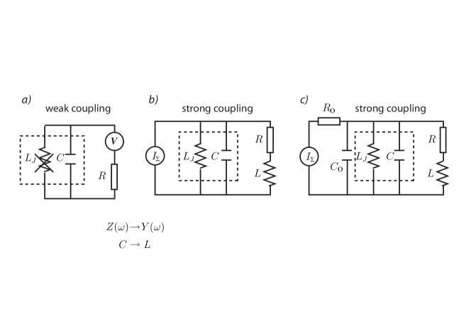
Figure 3: Strong coupling limit and environment duality. The dashed squares show the circuit elements, which present the Josephson and the noise junctions with the capacitance $C=C_{J}+C_{s}$. The current source $I_{\Sigma}=I+I_{s}$ provides the constant current $I$ and the noisy current $I_{s}$ in parallel. a) The dual weak-coupling case. The inductance $L_{J}$ of the Josephson junction is negligible in the weak-coupling limit. b) The dual strong-coupling limit. c) The strong-coupling case taking into account the capacitance $C_{0}$ and the resistance $R_{0}$ of the leads.

In the case of equilibrium noise the strong coupling limit can be investigated using the duality relations, which connect the parameters of the Josephson junction in the weak coupling and the strong coupling limits SZ ; Weiss :

$$E_{J}\rightarrow 2\Delta~{},~{}~{}V\rightarrow{h\over 4e^{2}}I=R_{Q}I~{},~{}~{}\varphi\rightarrow{\pi Q\over e}~{},~{}~{}~{}\rho={R\over R_{Q}}\rightarrow\tilde{\rho}={R_{Q}\over R}~{},~{}~{}~{}Z\rightarrow Y~{}.$$ (78)

Here $Y(\omega)$ is the admittance of the electric circuit, and $\Delta$ is the matrix element for a transition between adjacent states of the Josephson junction with localized phases $2\pi n$ and $2\pi(n+1)$ ($\hbar/\Delta$ is the life time at the state, which corresponds to some localized phase). Using these relations the $IV$ curve in the weak coupling limit, Eq. (7), transforms to the dual $VI$ curve in the strong-coupling limit:

$$V=-{4\pi\Delta^{2}\over e\hbar}\int_{0}^{\infty}dt\mbox{Im}\left\{e^{\tilde{J}_{0}(t)}\right\}\sin\left(2eR_{Q}It\over\hbar\right)=-{4\pi\Delta^{2}\over e\hbar}\int_{0}^{\infty}dt\mbox{Im}\left\{e^{\tilde{J}_{0}(t)}\right\}\sin\left(\pi It\over e\right)~{}.$$ (79)

The charge-charge correlator [see Eq. (149) in Ref. IN, ] is given by the relation dual to Eq. (5):

$$\tilde{J}_{0}(t)=2R_{Q}\int_{0}^{\infty}{d\omega\over\omega}{\mbox{Re}Y(\omega)}\left[\coth\left({1\over 2}\beta\hbar\omega\right)(\cos\omega t-1)-i\sin\omega t\right]~{}.$$ (80)

In order to exploit duality completely, i.e., not only for the general expression for the $IV$ curve but also for the specific results for ohmic environment with the effective impedance $Z=(1/R+i\omega C)^{-1}$, one should find a corresponding “dual” environment for the strong-coupling case. In the weak-coupling case the finite relaxation time $\tau=RC$ is provided by the imaginary element of the impedance $Z$, which is the capacitance $C=C_{J}+C_{s}$ of the two junctions (without the noise source $C_{s}=0$). In the strong coupling case the both imaginary elements of the Josephson junction (capacitance and inductance) do not contribute to the admittance (see Fig. 3b). In order to get a finite relaxation time dual to the time $\tau=RC$ of the weak coupling limit one should add to the effective electric circuit the inductance $L$ in series with the ohmic shunt resistance $R$ (Fig. 3b). Then the admittance dual to the impedance $Z$ of the weak coupling limit is

$$Y(\omega)=\frac{1}{R+i\omega L}=\frac{1/R}{1+i\omega\tau_{L}}~{},$$ (81)

where the circuit relaxation time $\tau_{L}=L/R$ is dual to the relaxation time $\tau=RC$ in the weak coupling limit. Thus duality relations Eq. (78) should by supplemented by the “environment duality” relation $C\rightarrow L$. Note, however, that introduction of finite inductance $L$ is not the only way to achieve a finite relaxation time. For example, Schön and Zaikin SZ suggested that the period of Josephson plasma oscillation $\sim\hbar/\sqrt{E_{J}E_{c}}$ should play the role of relaxation time dual to the time $RC$ in the weak coupling limit.

V.2 With shot noise

The duality concept is valid only for equilibrium noise when symmetry between current and voltage or impedance and admittance takes place. In the case of shot noise this symmetry is broken since shot noise is a current noise, which produces asymmetric effects on the current and on the voltage. Though we can still use the duality for description of the equilibrium contribution to the noise (this contribution cannot be ignored even if our goal is the effect of shot noise), the effect of shot noise on the $IV$ curve is essentially different in the weak and the strong coupling limits.

In the strong-coupling limit the effect of environment is governed by charge fluctuations. Whereas the phase fluctuations were determined by the voltage fluctuations via the Josephson relation $\hbar d\varphi/dt=2eV$, the charge fluctuations are determined by the current fluctuations via the relation $dQ/dt=I$. Important is that the current $I$ should be the total current of the part of the circuit, which describes the Josephson junction in the RCSJ model (inductance + capacitance + shunt resistance). Single-electron tunneling through the noise junction produces a pulse of the total current. If the tunneling time is very short, the pulse can be approximated by the $\delta$-function current peak. The effective circuit in Fig. 3b cannot broaden the original $\delta$-function current peak. This is in contrast to the voltage pulses, which were relevant for phase fluctuations in the weak coupling limit: the $\delta$-function current peak produced the voltage pulse of width $\tau=RC$. Meanwhile, the finite width of the current pulse is of principal importance for the shot-noise effect and therefore cannot be ignored. Broadening of the current pulse can be determined by additional lump elements of the electric circuit, which are connected with the ohmic resistance $R_{0}$ and the capacitance $C_{0}$ of wires connecting the current-noise source and the probe Josephson junction (see Fig. 3c). Bearing in mind this electric circuit the single-electron tunneling at $t-0$ produces the current pulse

$$\delta I(t)=\mbox{sign}(I_{s}){e\over\tau_{s}}e^{-t/\tau_{s}}~{},$$ (82)

which brings the charge

$$\delta Q_{s}(t)=\mbox{sign}(I_{s})e(1-e^{-t/\tau_{s}})~{}.$$ (83)

Here $\tau_{s}=R_{0}C_{0}$. The $VI$ curve with shot noise is given by

$$V=-{4\pi\Delta^{2}\over e\hbar}\int_{0}^{\infty}dt\mbox{Im}\left\{e^{\tilde{J}_{0}(t)}\right\}\left\langle\sin\left({\pi It\over e}+{\pi\Delta Q_{s}\over e}\right)\right\rangle~{},$$ (84)

where $\Delta Q_{s}=Q_{s}(t_{0})-Q_{s}(t_{0}-t)$ and

$$Q_{s}(t)=\mbox{sign}(I_{s})\pi\sum_{i}\Theta(t-t_{i})\left[1-e^{-(t-t_{i})/\tau}\right]~{}.$$ (85)

The shot-noise charge-charge correlators are found by averaging over the the time $t_{0}$. The expressions for $\langle\cos(\pi\Delta Q_{s}/e)\rangle$ and $\langle\sin(\pi\Delta Q_{s}/e)\rangle$ follow from those for $\langle\cos(\Delta\varphi_{s})\rangle$ and $\langle\sin(\Delta\varphi_{s})\rangle$ assuming $\rho=1$ and using the duality relations between the phase and the charge:

$${e\over I_{s}\tau_{s}}\left\langle\sin{\pi\Delta Q_{s}\over e}\right\rangle=\mbox{si}\pi-\mbox{si}\left(\pi e^{-t/\tau_{s}}\right)+\mbox{si}\left[\pi\left(1-e^{-t/\tau_{s}}\right)\right]+{\pi\over 2}~{},$$ (86)

$${e\over|I_{s}|\tau_{s}}\left(\left\langle\cos{\pi\Delta Q_{s}\over e}\right\rangle-1\right)=-\mbox{ci}\pi+\mbox{ci}\left(\pi e^{-t/\tau_{s}}\right)-{t\over\tau_{s}}+\mbox{ci}\left[\pi\left(1-e^{-t/\tau_{s}}\right)\right]-\gamma-\ln\left[\pi\left(1-e^{-t/\tau_{s}}\right)\right]~{}.$$ (87)

In contrast to the weak-coupling case where the single relaxation time $\tau$ characterized both the equilibrium and the shot-noise correlators, in the strong coupling case the equilibrium charge correlator is characterized by the time $\tau_{L}$, whereas the shot-noise charge correlator has the other characteristic time $\tau_{s}$. We expect that $\tau_{s}\ll\tau_{L}$. Therefore we should consider the limit $t\gg\tau_{s}$ in Eqs. (86) and (87):

$$\left\langle\sin{\pi\Delta Q_{s}\over e}\right\rangle=(2\mbox{si}\pi+\pi){I_{s}\over e}\tau_{s}=3.704{I_{s}\over e}\tau_{s}~{},$$ (88)

$$\left\langle\cos{\pi\Delta Q_{s}\over e}\right\rangle-1=-2{|I_{s}|\over e}t~{}.$$ (89)

We expand the shot noise contribution with respect to the current $I$:

$$\Delta V=-{4\pi\Delta^{2}\over e\hbar}\int_{0}^{\infty}dt\mbox{Im}\left\{e^{\tilde{J}_{0}(t)}\right\}\left[\sin\left({\pi It\over e}\right)\left(\left\langle\cos{\pi\Delta Q_{s}\over e}\right\rangle-1\right)+\cos\left({\pi It\over e}\right)\left\langle\sin{\pi\Delta Q_{s}\over e}\right\rangle\right]$$

$$\approx-{4\pi\Delta^{2}\over e\hbar}\int_{0}^{\infty}dt\mbox{Im}\left\{e^{\tilde{J}_{0}(t)}\right\}\left[{\pi It\over e}\left(\left\langle\cos{\pi\Delta Q_{s}\over e}\right\rangle-1\right)+\left\langle\sin{\pi\Delta Q_{s}\over e}\right\rangle\right]=V_{0}+R_{s}I~{}.$$ (90)

Rotating the integration path in the complex plane ($t\to-iy$) we obtain the ratchet voltage $V_{0}$ and the zero-bias resistance $R_{s}$:

$$V_{0}=-{4\pi\Delta^{2}\over e\hbar}\int_{0}^{\infty}dt\mbox{Im}\left\{e^{\tilde{J}_{0}(t)}\right\}\left\langle\sin{\pi\Delta Q_{s}\over e}\right\rangle$$

$$=-{14.8\pi\Delta^{2}\over e^{2}\hbar}I_{s}\tau_{s}\int_{0}^{\infty}dt\mbox{Im}\left\{e^{\tilde{J}_{0}(t)}\right\}={14.8\pi\Delta^{2}\over e^{2}\hbar}I_{s}\tau_{s}\int_{0}^{\infty}dye^{-\pi\tilde{\rho}y/\tau_{L}}={14.8\Delta^{2}\over e^{2}\hbar}{\tau_{L}\over\tilde{\rho}}I_{s}\tau_{s}={7.4\pi\Delta^{2}\over e^{4}}{L\tau_{s}\over R_{Q}^{2}}I_{s}~{},$$ (91)

$$R_{s}=-{4\pi^{2}\Delta^{2}\over e^{2}\hbar}\int_{0}^{\infty}t\,dt\mbox{Im}\left\{e^{\tilde{J}_{0}(t)}\right\}\left(\left\langle\cos{\pi\Delta Q_{s}\over e}\right\rangle-1\right)$$

$$=|I_{s}|{8\pi^{2}\Delta^{2}\over e^{3}\hbar}\int_{0}^{\infty}t^{2}\,dt\mbox{Im}\left\{e^{\tilde{J}_{0}(t)}\right\}=|I_{s}|{8\pi^{2}\Delta^{2}\over e^{3}\hbar}\int_{0}^{\infty}y^{2}\,dye^{-\pi\tilde{\rho}y/\tau_{L}}=|I_{s}|{16\pi^{2}\Delta^{2}\over e^{3}\hbar}\left(\tau_{L}\over\pi\tilde{\rho}\right)^{3}=|I_{s}|{8\Delta^{2}\over e^{5}}{L^{3}\over R_{Q}^{4}}~{}.$$ (92)

One can see that the even effect (resistance $R_{s}$) remains finite in the limit $\tau_{s}\to 0$. In contrast, the ratchet effect, which is an odd effect, vanishes. More generally, any odd effect should vanish in the limit $\tau_{s}\to 0$. This is because in this limit tunneling events lead to instantaneous transfers of charge $\pm e$. The odd effect should depend on the sign of transferred charge, but the current cannot depend on whether the charge $+e$ or $-e$ suddenly appears at the Josephson junction due to periodicity of the charge correlator with the period $2e$: the instantaneous transfers of the charges $+e$ and $-e$ must produce identical effects. Only finite duration of the current pulse (finite $\tau_{s}$) can lead to an odd effect (ratchet voltage $V_{0}$ as an example).

This interesting feature of the strong-coupling case becomes even more pronounced if shot noise originates from the current of Cooper pairs. This can be realized if the noise junction is a SIN junction in the regime of the Andreev reflection or a Josephson junction in the weak coupling limit in the regime of incoherent tunneling of Cooper pairs. In the both cases the tunneling event is accompanied by the charge jump $Q_{s}=2e(1-e^{-t/\tau_{s}})\mbox{sign}(I_{s})$ and, in analogy with Eqs. (86) and (87), the odd and the even charge correlators can be obtained from the phase-phase correlators using duality and assuming $\rho=2$:

$${e\over I_{s}\tau_{s}}\left\langle\sin{\pi\Delta Q_{s}\over e}\right\rangle=-\mbox{si}(2\pi)+\mbox{si}\left(2\pi e^{-t/\tau_{s}}\right)+\mbox{si}\left[2\pi\left(1-e^{-t/\tau_{s}}\right)\right]+{\pi\over 2}~{},$$ (93)

$${e\over|I_{s}|\tau_{s}}\left(\left\langle\cos{\pi\Delta Q_{s}\over e}\right\rangle-1\right)=\mbox{ci}(2\pi)-\mbox{ci}\left(2\pi e^{-t/\tau_{s}}\right)-{t\over\tau_{s}}+\mbox{ci}\left[2\pi\left(1-e^{-t/\tau_{s}}\right)\right]-\gamma-\ln\left[2\pi\left(1-e^{-t/\tau_{s}}\right)\right]~{}.$$ (94)

In the limit $t\gg\tau_{s}$

$${e\over I_{s}\tau_{s}}\left\langle\sin{\pi\Delta Q_{s}\over e}\right\rangle=2\pi e^{-t/\tau_{s}}~{},$$ (95)

$${e\over|I_{s}|\tau_{s}}\left(\left\langle\cos{\pi\Delta Q_{s}\over e}\right\rangle-1\right)=2[\mbox{ci}(2\pi)-\gamma-\ln(2\pi)]+\pi^{2}e^{-2t/\tau_{s}}~{}.$$ (96)

Calculating the shot-noise contribution to the voltage one cannot expand in $t/\tau_{s}$ but can expand in $t/\tau_{L}$ and in the current $I$:

$$\Delta V=-{4\pi\Delta^{2}\over e\hbar}\int_{0}^{\infty}dt\mbox{Im}\left\{e^{\tilde{J}_{0}(t)}\right\}\left[\left(\left\langle\cos{\pi\Delta Q_{s}\over e}\right\rangle-1\right))\sin\left({\pi It\over e}\right)+\left\langle\sin{\pi\Delta Q_{s}\over e}\right\rangle\cos\left({\pi It\over e}\right)\right]$$

$$\approx{4\pi^{2}\Delta^{2}\over e\hbar}{\tilde{\rho}\over\tau_{L}}\int_{0}^{\infty}t\,dt\left[\left(\left\langle\cos{\pi\Delta Q_{s}\over e}\right\rangle-1\right){\pi It\over e}+\left\langle\sin{\pi\Delta Q_{s}\over e}\right\rangle\right]=V_{0}+R_{s}I~{}.$$ (97)

Integrating by parts one obtains the ratchet voltage

$$V_{0}={4\pi^{2}\Delta^{2}\over e\hbar}{\tilde{\rho}\over\tau_{L}}\int_{0}^{\infty}t\,dt\left\langle\sin{\pi\Delta Q_{s}\over e}\right\rangle={8\pi^{3}\Delta^{2}\over e^{2}\hbar}{\tilde{\rho}\over\tau_{L}}I_{s}\int_{0}^{\infty}e^{-t/\tau_{s}}{t^{2}\over 2}\,dt\left\{\mbox{si}^{\prime}(2\pi e^{-t/\tau_{s}})\right.$$

$$\left.-\mbox{si}^{\prime}\left[2\pi\left(1-e^{-t/\tau_{s}}\right)\right]\right\}={2\pi^{2}\Delta^{2}\over e^{2}\hbar}{\tilde{\rho}\over\tau_{L}}I_{s}\tau_{s}^{3}\int_{0}^{\infty}x^{2}\,dx\left[\sin(2\pi e^{-x})-{\sin\left[2\pi\left(1-e^{-x}\right)\right]\over e^{x}-1}\right]={7.62\pi^{3}\Delta^{2}\tau_{s}^{3}\over e^{4}L}I_{s}~{},$$ (98)

and the short noise contribution to the zero-bias resistance

$$R_{s}={4\pi^{3}\Delta^{2}\over e^{2}\hbar}{\tilde{\rho}\over\tau_{L}}\int_{0}^{\infty}t^{2}\,dt\left(\left\langle\cos{\pi\Delta Q_{s}\over e}\right\rangle-1\right)=-{4\pi^{3}\Delta^{2}\over e^{3}\hbar}{\tilde{\rho}\over\tau_{L}}|I_{s}|\int_{0}^{\infty}{t^{3}\over 3}\,dt\left[\mbox{ci}^{\prime}(2\pi e^{-t/\tau_{s}})2\pi e^{-t/\tau_{s}}-1\right.$$

$$\left.+\mbox{ci}^{\prime}\left[2\pi\left(1-e^{-t/\tau_{s}}\right)\right]2\pi e^{-t/\tau_{s}}-{e^{-t/\tau_{s}}\over 1-e^{-t/\tau_{s}}}\right]$$

$$={4\pi^{3}\Delta^{2}\tau_{s}^{4}\over 3e^{3}\hbar}{\tilde{\rho}\over\tau_{L}}|I_{s}|\int_{0}^{\infty}x^{3}\,dx\left[1-\cos(2\pi e^{-x})+{1-\cos\left[2\pi\left(1-e^{-x}\right)\right]\over e^{x}-1}\right]={5.08\pi^{4}\Delta^{2}\tau_{s}^{4}\over e^{5}L}|I_{s}|~{}.$$ (99)

Thus shot noise from the current of Cooper pairs produces neither odd nor even effects if duration $\tau_{s}$ of a single current pulse vanishes.

What would happen if experimentalists were able to decrease the time $\tau_{s}$ essentially? Eventually this time would be comparable or even less that the intrinsic time, which determines duration of single-electron tunneling. Then the experimental observation of the zero-bias anomaly would provide an information on this intrinsic time. Up to now the tunneling time is mostly an issue of theoretical debates trav ; Hauge ; Land : Though some attempts to observe it were undertaken, but their interpretation is ambiguous (see Ref. Land, and references therein). The subject is controversial and the consensus on how this time should be defined is absent. Decreasing of $R_{0}$ and $C_{0}$ the experimentalists would shift this issue from the pure theory to the measurement. How realistic could this perspective be? Presently it is difficult to achieve $R_{0}$ less than 100 $\Omega$ and $C_{0}$ less then 1 fF. This yields $\tau_{s}=R_{0}C_{0}>10^{-13}$ s. On the other hand, whatever disagreement on definition of the tunneling time, usually it is estimated as $10^{-15}~{}-~{}10^{-14}$ s. This yields the hope that further progress in miniaturization of the experimental set up or searching for cases with longer tunneling time could open a new possibility to investigate the tunneling time experimentally.

VI Conclusions

We have presented the theory of the effect of shot noise from an independent source on the Coulomb blockaded Josephson junction in high-impedance environment. The analysis takes into account asymmetry of shot noise characterized by its odd moments. For high impedance environment the effect is so strong that the expansion in moments is not valid and was not used in the analysis. Asymmetry of shot noise results in asymmetry of the $IV$ curve: the shift of the conductance minimum from the zero bias and the ratchet effect, which have been observed experimentally SN ; exp . At low noise currents (currents responsible for shot noise) the effect is proportional to the noise current independently of counting statistics of electron transport. However, at high noise currents the effect of noise on the $IV$ curve is very sensitive to electron counting statistics. This high sensitivity is explained by the fact that in contrast to usual methods of noise detection the Coulomb blockaded junction probes phase but not voltage.

The theory was generalized on another type of noise (phase noise of a monochromatic AC input) and on a normal Coulomb blockaded tunnel junction, In the both cases the effect of noise strongly affects the Coulomb zero-bias anomaly of the $IV$ curve. The effect of shot noise on the superconducting Josephson junction in low-impedance environment was also considered. If environment generates only the equilibrium Johnson-Nyquist noise this case can be analyzed using the duality relations with the case of the Coulomb blockaded Josephson junction in high-impedance environment. However, shot noise breaks duality relations between the two cases. An interesting feature of the superconducting Josephson junction in low-impedance environment has been revealed: the effect of shot noise on its $IV$ curve can give information on the time of electron tunneling through the junction responsible for shot noise.

Altogether, the analysis demonstrates, that the low-bias part of the $IV$ curves of tunnel junctions, both Coulomb blockaded and superconducting, can be exploited as a sensitive detector of various types of noise.

References

• (1) Ya.M. Blanter and M. BΓΌttiker, Phys. Rep. 336, 1 (2000).
• (2) G.B. Lesovik, Pis’ma Zh. Eksp. Teor. Fiz. 60, 806 (1994)[JETP Lett. 60, 820 (1994)].
• (3) L.S. Levitov, H. Lee, and G.B. Lesovik, J. Math. Phys. 37, 4845 (1996); L.S. Levitov and M. Reznikov, Phys. Rev. B 70, 115305 (2004); A. Shelankov and J. Rammer, Europhys. Lett. 63, 485 (2003); D.B. Gutman and Y. Gefen, Phys. Rev. B 68, 035302 (2003).
• (4) C.W.J. Beenakker, M. Kindermann, and Yu.V. Nazarov, Phys. Rev. Lett. 90, 176802 (2003).
• (5) B. Reulet, J. Senzier, and D.E. Prober, Phys. Rev. Lett. 91, 196601 (2003); B. Reulet, cond-mat/0502077.
• (6) Yu. Bomze, G. Gershon, D. Shovkun, L.S. Levitov, and M. Reznikov, cond-mat/0504382.
• (7) J. Delahaye, R. Lindell, M.S. SillanpÀÀ, M.A. Paalanen, E.B. Sonin, and P.J. Hakonen, cond-mat/0209076 (unpublished).
• (8) R. Lindell, J. Delahaye, M.A. SillanpÀÀ, T.T. HeikkilΓ€, E.B. Sonin, and P.J. Hakonen, Phys. Rev. Lett. 93, 197002 (2004).
• (9) E. B. Sonin, Phys. Rev. B 70, 140506(R) (2004).
• (10) T.T. HeikkilΓ€, P. Virtanen, G. Johansson, and F.K. Wilhelm, Phys. Rev. Lett. 93, 247005 (2004).
• (11) R. Deblock, E. Onak, L. Gurevich, and L.P. Kouwenhoven, Science 301, 203 (2003); cond-mat/0405601.
• (12) J. Tobiska and Yu.V. Nazarov, Phys.Rev. Lett. 93, 106801 (2004).
• (13) J.P. Pekola, Phys.Rev. Lett. 93, 206601 (2004); J.P. Pekola, T.E. Nieminen, M. Meschke, J.M. Kivioja, A.O. Niskanen, and J.J. Vartiainen, cond-mat/0502446.
• (14) J. Ankerhold and H. Grabert, cond-mat/0504120.
• (15) D.V. Averin, Yu.V. Nazarov, and A.A. Odintsov, Physica B 165&166, 945 (1990).
• (16) G. SchΓΆn and A.D. Zaikin, Phys. Rep. 198, 237 (1990).
• (17) G.L. Ingold and Yu.V. Nazarov, in Single Charge Tunneling, Coulomb Blockade Phenomena in Nanostructures, ed. by H. Grabert and M. Devoret (Plenum, New York, 1992), pp. 21-107.
• (18) M. Abramowitz and I. A. Stegun, Handbook of Mathematical Functions (Dover, New York, 1972).
• (19) G.-L. Ingold, H. Grabert, and U. Eberhardt, Phys.Rev. B 50, 395 (1994); G.-L. Ingold and H. Grabert, Phys.Rev. Lett. 83, 3721 (1999).
• (20) R. Loudon, The Quantum Theory of Light, (Oxford Univ. Press, 2000).
• (21) G. Falci, V. Bubanja, and SchΓΆn, Z. Phys. B–Condensed Matter 85, 451 (1991).
• (22) A.A. Odintsov, G. Falci, and G. SchΓΆn, Phys. Rev. B 44, 13 089 (1991); P. Joyez and D. Esteve, Phys. Rev. B 56, 1848 (1997).
• (23) U. Weiss, Quantum Dissipative Systems, (World Scientific, Singapur, 1999).
• (24) M. BΓΌttiker and R. Landauer, IBM J. Res. Dev. 30, 451 (1986).
• (25) E.H. Hauge and J.A. StΓΈvneng, Rev. Mod. Phys. 61, 917 (1989).
• (26) R. Landauer, Rev. Mod. Phys. 66, 217 (1994).