Shell structure in the density profile of a rotating gas of spin-polarized fermions

Abstract

We present analytical expressions and numerical illustrations for the ground-state density distribution of an ideal gas of spin-polarized fermions moving in two dimensions and driven to rotate in a harmonic well of circular or elliptical shape. We show that with suitable choices of the strength of the Lorentz force for charged fermions, or of the rotational frequency for neutral fermions, the density of states can be tuned as a function of the angular momentum so as to display a prominent shell structure in the spatial density profile of the gas. We also show how this feature of the density profile is revealed in the static structure factor determining the elastic light scattering spectrum of the gas.

1 Introduction

Ultracold Fermi gases of alkali atoms such as ⁴⁰K or ⁶Li in harmonic traps are quantum systems that are experimentally accessible by the techniques of atom trapping and cooling [1, 2]. The high purity and the low temperature of the samples and the high resolution of the detection techniques make these systems ideal candidates for the study on the mesoscopic scale of single-level quantum properties such as shell structures in the particle density profiles [3, 4, 5, 6, 7]. In the experiments the trapped atomic gas can be fully spin-polarized and the strength and the anisotropy of the trap can be tuned to reach quasi-onedimensional (1D) or quasi-twodimensional (2D) configurations. Quantum effects in the equilibrium profiles can be greatly enhanced by varying the anisotropy of the confinement [6]. Here we show how to enhance quantum effects on 2D equilibrium density profiles by putting the gas into rotation.

In a wholly different physical realm electrons in a quantum dot realize a Fermi gas moving in a plane under the effect of a harmonic potential. A quantum dot is often described as an artificial atom, in which a confinement potential replaces the attractive potential of the nucleus and the increased length scale allows access to experiments that are not practicable on real atoms [8, 9, 10]. Spin effects are also accessible and complete spin polarization is easily achieved in a small dot. Confinement by a circularly symmetric harmonic potential is of special interest, since in this case the energy needed to add electrons to the dot reveals a shell structure [11]. The effects of a magnetic field on the electronic properties of circular quantum dots have been studied by numerical diagonalization and by spin-density functional methods (see Ref. [12] and references therein). These approaches have also been applied to rectangular dot structures, when the effective lateral confinement is described as elliptical. In such a confinement the single-particle energy levels as well as the energy spectra for two-electron systems are exactly known as functions of the magnetic field [13, 14].

A Fermi gas of spin-polarized charged particles in a uniform magnetic field, under conditions such that the Coulomb interactions can be neglected as specified below, can be mapped into a rotating Fermi gas of neutral atomic particles in a state of complete spin polarization, where the atom-atom interactions are negligible on account of the Pauli principle suppressing $s$-wave scattering. In this work we examine the particle density profiles of the ideal system that we have just introduced. For definiteness we shall refer throughout the paper to the ideal 2D Fermi gas of charged particles in a uniform magnetic field, although some parts of the discussion (and in particular the analysis of the elastic light scattering spectrum given in Sec. 4) are specifically aimed at an atomic Fermi gas in uniform rotation.

An ideal 2D Fermi gas of charged particles in a uniform magnetic field has recently been studied by van Zyl and Hutchinson [15], who have used an inverse Laplace transform method and an expansion in Laguerre polynomials to calculate its thermodynamic properties. Their method can be implemented exactly in the case of a uniform gas, whereas recourse to a local-density approximation is needed for an inhomogeneous gas on account of the broken symmetry induced by the concurrent effects of the harmonic confinement and of the magnetic field. However, the single-particle Hamiltonian of the ideal gas can be diagonalized on the basis of left and right circular or elliptical quanta, bringing it to the form of the Hamiltonian of two independent harmonic oscillators. The eigenfunctions can thus be written in terms of Hermite polynomials, as we do in this work. Practical applications of our approach are limited to ultracold Fermi gases consisting of a restricted number of particles, so that the number of Hermite polynomials that need explicit numerical calculation remains limited. We shall give below numerical illustrations for systems of 10 and 106 fermions at zero temperature.

The paper is organized as follows. In Sec. 2 we set out the single-particle Hamiltonian of the system in a generic gauge which allows its diagonalization on the basis of left and right-handed circular or elliptical quanta. In Sec. 3 we express the spatial density profile of the gas in terms of Hermite polynomials and display several configurations for various values of the strength of the magnetic field and of the anisotropy parameters of the confinement. We show that an impressive shell structure arises in the profile whenever there is an excess of density of states with zero angular momentum. In Sec. 4 we calculate the elastic contribution to the static structure factor of the gas, in order to show how the shell structure is reflected in the elastic light scattering spectrum. Finally Sec. 5 offers some concluding remarks.

2 The model

We consider a 2D spin-polarized Fermi gas at zero temperature, made up of $N$ non-interacting fermions of charge $e$ and mass $m_{f}$ subject to a uniform magnetic field ${\bf B}=\boldsymbol{\nabla}\times{\bf A}$ perpendicular to the plane of confinement (the $\{x,y\}$ plane, say). The gas is immersed in a uniformly charged background medium so that the total system is neutral. Screening effects cut the range of the Coulomb interactions and to a first approximation these can be neglected on account of the Pauli principle keeping fermions with parallel spins far apart from each other. More generally, the Coulomb interactions between electrons in a quantum dot are negligible when the harmonic oscillator length characterizing the confinement is small compared with the effective Bohr radius.

As already noted in Sec. I, this system can be mapped into a spin-polarized gas of $N$ neutral fermions confined in a rotating trap. The map is guaranteed by a correspondence between the Maxwell equations and the Navier-Stokes equations in the absence of viscosity, as demonstrated by Marmanis [16]. In the rotating system the velocity field ${\bf v}$ of the fermions and the vorticity $\boldsymbol{\omega}=\boldsymbol{\nabla}\times{\bf v}$ play the role of the vector potential ${\bf A}$ and of the magnetic field ${\bf B}$, respectively.

2.1 Circular trap

It is useful to present first the case of an isotropic harmonic potential. The single-particle Hamiltonian for non-interacting fermions is

$$\hat{H}=\dfrac{1}{2m_{f}}(\hat{p}_{x}^{2}+\hat{p}_{y}^{2})+\dfrac{1}{2}m_{f}[(\omega_{0}^{2}+\omega_{L}^{2})(\hat{x}^{2}+\hat{y}^{2})]+\omega_{L}(\hat{x}\hat{p}_{y}-\hat{p}_{x}\hat{y})\,.$$ (1)

In Eq. (1) ${\omega}_{0}$ is the trap frequency, $\omega_{L}=eB/(2cm_{f})$ is the Larmor frequency, and we have chosen the symmetric gauge for the vector potential ${\bf A}=(-{By}/2,{Bx}/2,0)$, as is suited to the circular symmetry of the confinement [17].

The Hamiltonian (1) is separable [18] upon introducing first the creation and destruction operators $\hat{a}_{x,y}^{\dagger}$ and $\hat{a}_{x,y}$ for a quantum of oscillation in the $x$ or $y$ direction, defined according to $\hat{a}_{x}=[(\hbar/m_{f}\Omega)^{-1/2}\hat{x}+i(\hbar m_{f}\Omega)^{-1/2}\hat{p}_{x}]/\sqrt{2}$ where $\Omega=(\omega_{0}^{2}+\omega_{L}^{2})^{1/2}$, and then the operators $\hat{a}_{d}=(\hat{a}_{x}-i\hat{a}_{y})/\sqrt{2}$ and $\hat{a}_{g}=(\hat{a}_{x}+i\hat{a}_{y})/\sqrt{2}$. The transformed Hamiltonian is

$$\hat{H}=\hbar\omega_{d}\left(\hat{a}_{d}^{\dagger}\hat{a}_{d}+\dfrac{1}{2}\right)+\hbar\omega_{g}\left(\hat{a}_{g}^{\dagger}\hat{a}_{g}+\dfrac{1}{2}\right)$$ (2)

where $\omega_{d}=\Omega+\omega_{L}$ and $\omega_{g}=\Omega-\omega_{L}$.

The operator $\hat{a}_{d}$ ($\hat{a}_{g}$) can be interpreted as the destruction operator of a right (left) circular quantum, the number of such quanta being given by $\hat{n}_{d}=\hat{a}_{d}^{\dagger}\hat{a}_{d}$ ($\hat{n}_{g}=\hat{a}_{g}^{\dagger}\hat{a}_{g}$). The quantity $\hbar(\hat{n}_{d}-\hat{n}_{g})$ gives the eigenvalues of the angular momentum operator $\hat{L}_{z}=\hat{x}\hat{p}_{y}-\hat{y}\hat{p}_{x}$.

2.2 Elliptical trap

In the case of anisotropic 2D confinement neither the symmetric gauge nor the Landau gauge are useful. We write the single-particle Hamiltonian in the general form

$$\hat{H}=\dfrac{1}{2m_{f}}(\hat{p}_{x}-\alpha eB\hat{y}/c)^{2}+\dfrac{1}{2m_{f}}(\hat{p}_{y}+(1-\alpha)\,eB\hat{x}/c)^{2}+\dfrac{1}{2}m_{f}\omega_{0}^{2}(\hat{x}^{2}+\lambda^{2}\hat{y}^{2})$$ (3)

with $0<\alpha<1$ and $\lambda$ the anisotropy parameter. Equation (3) can be rewritten as

$$\hat{H}=\dfrac{1}{2m_{f}}(\hat{p}_{x}^{2}+\hat{p}_{y}^{2})+\dfrac{1}{2}m_{f}(\omega_{x}^{2}\hat{x}^{2}+\omega_{y}^{2}\hat{y}^{2})+2\omega_{L}\left[(1-\alpha)\hat{x}\hat{p}_{y}-\alpha\hat{p}_{x}\hat{y}\right]$$ (4)

where we have set $\omega_{x}^{2}=\omega_{0}^{2}+4(1-\alpha)^{2}\omega_{L}^{2}$ and $\omega_{y}^{2}=\lambda^{2}\omega_{0}^{2}+4\alpha^{2}\omega_{L}^{2}$. By imposing the condition $(1-\alpha)/{\alpha}={\omega_{x}(\alpha)}/{\omega_{y}(\alpha)}$, which has the solution

$$\alpha=\lambda/(1+\lambda)\,,$$ (5)

and using $\hat{a}_{x}=[(\hbar/m_{f}\omega_{x})^{-1/2}\hat{x}+i(\hbar m_{f}\omega_{x})^{-1/2}\hat{p}_{x}]/\sqrt{2}$ etcetera, Eq. (4) becomes

$$\hat{H} = \dfrac{1}{2}\hbar\left(\omega_{x}+\omega_{y}\right)(\hat{a}_{x}^{\dagger}\hat{a}_{x}+\hat{a}_{y}^{\dagger}\hat{a}_{y}+1)+\dfrac{1}{2}\hbar\left(\omega_{x}-\omega_{y}\right)(\hat{a}_{x}^{\dagger}\hat{a}_{x}-\hat{a}_{y}^{\dagger}\hat{a}_{y})$$ (6)

$$+ 2\dfrac{\sqrt{\lambda}}{1+\lambda}i\hbar\omega_{L}\left[\hat{a}_{x}\hat{a}_{y}^{\dagger}-\hat{a}_{x}^{\dagger}\hat{a}_{y}\right]\,.$$

For circular confinement ($\lambda=1$) the $\alpha$-gauge given by the relation in Eq. (5) reduces to the symmetric gauge, while in the limit of one-dimensional confinement ($\lambda=0$ or $\infty$) it reduces to the Landau gauge. More generally, in the mapping with a rotating system the $\alpha$-gauge corresponds to a velocity field which follows the symmetry of the confinement.

The Hamiltonian in Eq. (6) is separable in terms of the operators

$$\left\{\begin{array}[]{l}\hat{a}_{d}=\cos\theta\,\hat{a}_{x}-i\sin\theta\,\hat{a}_{y}\\ \hat{a}_{g}=\sin\theta\,\hat{a}_{x}+i\cos\theta\,\hat{a}_{y}\\ \end{array}\right.$$ (7)

if the angle $\theta$ satisfies the relation $\tan(2\theta)=2\tilde{\omega}_{L}/(\omega_{x}-\omega_{y})$, with $\tilde{\omega}_{L}=2\sqrt{\lambda}\omega_{L}/(1+\lambda)$. In the new basis the Hamiltonian can be written as in Eq. (2) with

$$\omega_{d,g}=\dfrac{1}{2}(\omega_{x}+\omega_{y})\pm\sqrt{\tilde{\omega}_{L}^{2}+\dfrac{1}{4}(\omega_{x}-\omega_{y})^{2}}$$ (8)

The operators $\hat{a}_{d}$ and $\hat{a}_{g}$ are the destruction operators for a right-handed and a left-handed elliptical quantum, but (if $\theta\neq\pi/4$) the quantum number $m=n_{d}-n_{g}$ is no longer proportional to the angular momentum $L_{z}$.

3 Spatial density profiles

The eigenstate $|\chi_{n_{d},n_{g}}\rangle$ corresponding to the occupation numbers $\{n_{d},n_{g}\}$ can be obtained by recursively applying the operators $\hat{a}^{\dagger}_{d}$ and $\hat{a}^{\dagger}_{g}$ to the ground state $|\chi_{0,0}\rangle$. Using Eq. (7) we can write

$$|\chi_{n_{d},n_{g}}\rangle=\dfrac{1}{\sqrt{n_{d}!n_{g}!}}(\cos\theta\hat{a}_{x}^{\dagger}+i\sin\theta\hat{a}_{y}^{\dagger})^{n_{d}}(\sin\theta\hat{a}_{x}^{\dagger}-i\cos\theta\hat{a}_{y}^{\dagger})^{n_{g}}|\chi_{0,0}\rangle\,,$$ (9)

where

$$\langle x,y|\chi_{0,0}\rangle=\pi^{-1/2}\exp(-x^{2}/2l_{x}^{2})\exp(-y^{2}/2l_{y}^{2})$$ (10)

with $l_{x,y}=\sqrt{\hbar/m_{f}\omega_{x,y}}$. Series expansion of Eq. (9) and use of the expression of the eigenstates of the harmonic oscillator in terms of Hermite polynomials lead to the result

$$\begin{split}\chi_{n_{d},n_{g}}(x,y)&=\dfrac{\exp(-x^{2}/2l_{x}^{2})\exp(-y^{2}/2l_{y}^{2})}{\sqrt{\pi\,l_{x}l_{y}\,2^{n_{d}+n_{g}}}}\sum_{j=0}^{n_{d}}\sum_{k=0}^{n_{g}}\dfrac{\sqrt{n_{d}!\,n_{g}!}}{j!(n_{d}-j)!k!(n_{g}-k)!}(-1)^{n_{g}-k}\\ &(i)^{n_{d}+n_{g}-k-j}(\sin\theta)^{n_{d}-j+k}(\cos\theta)^{n_{g}-k+j}H_{j+k}(x/l_{x})H_{n_{d}+n_{g}-j-k}(y/l_{y}).\\ \end{split}$$ (11)

Finally, the density profile $n(x,y)$ can be expressed in the form

$$n(x,y)=\sum_{n_{g}=0}^{N_{g}}\sum_{n_{d}=0}^{N_{d}}|\chi_{n_{d},n_{g}}(x,y)|^{2}\,.$$ (12)

Here,

$$N_{d}={\rm Int}\left[\frac{E_{F}}{\hbar\omega_{d}}-\left(n_{g}+\dfrac{1}{2}\right)\dfrac{\omega_{g}}{\omega_{d}}-\dfrac{1}{2}\right]\,$$ (13)

is the highest allowed value for the quantum number $n_{d}$ at given values of the Fermi energy $E_{F}$ and of the quantum number $n_{g}$, and

$$N_{g}={\rm Int}\left[\frac{E_{F}}{\hbar\omega_{g}}-\dfrac{\omega_{d}}{2\omega_{g}}-\dfrac{1}{2}\right]$$ (14)

is the highest allowed value for the quantum number $n_{g}$ at given $E_{F}$. Of course, the Fermi energy is determined by the number of fermions in the trap.

Figure 1 shows the particle density profile for 10 spin-polarized fermions in an isotropic trap ($\lambda=1$) at various strengths of the applied magnetic field, and Fig. 2 reports the corresponding density of occupied states (dos). In zero field (Figs. 1(a) and 2(a)) the total angular momentum is zero and the left and right states are equally populated. At a field strength such that the Larmor frequency is equal to the trap frequency (Figs. 1(b) and 2(b)) there still is an excess population of the state $m=0$ and a central peak in the density profile. At still higher fields (Figs. 1(c) and 2(c)) the dos becomes constant and the occupation of two states with opposite angular momentum ($m=\pm 1$) produces a central hole in the density profile. Finally, at very large fields (Figs. 1(d) and 2(d)) the Landau quantization limit is being recovered, with a filling factor equal to unity in a dos which is constant for $m\leq 0$. This is spatially the most compact distribution of the droplet of spin-polarized fermions, which is commonly denoted as MDD [19].

Similar density distributions can be obtained for higher numbers of fermions. In Fig. 3 we report as an example the spatial distribution of 106 fermions at $\omega_{L}=5\omega_{0}$, showing as in Fig. 1(b) a central peak from an excess dos at $m=0$. On a slight increase in the field strength, to $\omega_{L}\geq 5.1\omega_{0}$, the filling factor becomes unity and the density profile takes a MDD configuration similar to that shown in Fig. 1(d).

In an anisotropic trap the overall elliptical shape of the fermion cloud can still sustain a shell structure, which becomes progressively smoothen as the field is increased. In Fig. 4 we show the case of 10 fermions in a trap with anisotropy parameter $\lambda=4$. For $\omega_{L}=\omega_{0}$ (Fig. 4(b)) the dos is similar to that shown for a circular trap in Fig. 2(b), but the value of $m$ is not related to the angular momentum in the anisotropic trap and a central peak in the density profile is consequently missing. Instead, raising the field produces a softening of the oscillations of the profile along the x axis and some enhancement of those along the $y$ axis. This effect is more pronounced at $\omega_{L}=1.8\omega_{0}$ (Fig. 4(c)), where a central hole in the profile is accompanied by two bumps along the y axis. For this value of $\omega_{L}$ the dos is similar to that shown for a circular trap in Fig. 2(c). Again, all shell structures disappear and an MDD-like profile is obtained when the filling factor becomes unity (Fig. 4(d)).

Finally, Fig. 5 reports the density profile for 10 fermions in a strongly anisotropic trap ($\lambda=10$). In zero field (Fig. 5(a)) the system is quasi-onedimensional: only the ground state is occupied in the $y$ direction and density oscillations are present only along the $x$ axis. These become progressively smoothen as the field is applied (Fig. 5(b)) and increased (Fig. 5(c)).

4 Angular distribution of scattered light

The theory of light scattering from a confined cloud of spin-polarized fermionic atoms has been presented in Ref. [20]. Here we discuss an experiment of elastic scattering in which the incident beam is propagating along the $z$ direction, orthogonally to the $\{x,y\}$ plane of confinement of the gas.

The positive-frequency component of the incident electric field is

$${\bf E}_{F}^{+}(z,t)=\frac{1}{2}E\hat{\varepsilon}\exp[i(k_{L}z-\omega t)]$$ (15)

with $E$ and $\hat{\varepsilon}$ being the field amplitude and polarization vector, and ${k}_{L}$ and $\omega$ its wave number and frequency. The angular distribution of the scattered light can be decomposed into two components: an elastic term originating from diffraction by a finite object of given optical density profile, and an inelastic term determined by excitations in the quantum fluid. Only the elastic term remains if the light frequency is far-off-resonance from the internal states of the fluid. This term is determined by the elastic static structure factor $S_{e}(k_{x},k_{y})$, which is defined by

$$S_{e}(k_{x},k_{y})=\left|\int dx\int dy\,e^{-ik_{x}x}e^{-ik_{y}y}n(x,y)\right|^{2}$$ (16)

where ${\bf k}=({k}_{x},{k}_{y})$ is the wave vector transfer in the scattering process.

We have evaluated the elastic contribution to the static structure factor for the density distribution of 106 fermions shown in Fig. 3 and for a MDD configuration found with the same number of fermions at $\omega_{L}=5.1\omega_{0}$. These two configurations have essentially the same size and thus show almost identical central peaks in their diffraction pattern (see the inset in Fig. 6). According to Babinet’s principle this peak is given by the optical diffraction pattern of a circular aperture.

The central part of the density profile shown in Fig. 3 consists of a peak of diameter $\sim 2l_{x}$ surrounded by a ring of diameter $\sim 4l_{x}$. As noted in Sec. 3, this double structure arises from an excess of occupied states with zero angular momentum and its signal appears in the diffraction pattern in the range $1.5<k_{x}l_{x}<3$. In the same range the scattered intensity from the flat MDD configuration is much lower, as is seen in the main frame of Fig. 6.

5 Summary and conclusions

In summary, we have evaluated the particle density profiles of an ideal gas of spin-polarized fermions confined in 2D inside a circular or elliptical harmonic trap as functions of an applied magnetic field or of the trap rotational frequency. We have introduced a generic $\alpha$-gauge in which the eigenstates of the Hamiltonian can be expressed in terms of right-handed and left-handed elliptical quanta and written in terms of Hermite polynomials. The $\alpha$-gauge reduces to the symmetric gauge in a circular trap and to the Landau gauge in a strongly elongated trap.

In the case of a circular trap we have correlated the shell structures in the density profile of the gas with the density of occupied angular-momentum states and suggested that these structures may become observable in an elastic light scattering experiment from an atomic Fermi gas inside a rotating pancake-shaped trap. Other peculiar shell structures have been illustrated in the case of an elliptical trap. It remains a challenge to provide an exact treatment for a gas consisting of very large numbers of particles at finite temperature.

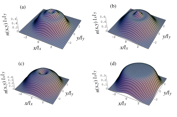
Figure 1: Density profile for 10 fermions in a circular harmonic trap at (a) $\omega_{L}$ = 0, (b) $\omega_{L}$ = $\omega_{0}$, (c) $\omega_{L}$ = 1.18$\omega_{0}$, and (d) $\omega_{L}$ = 10$\omega_{0}$.

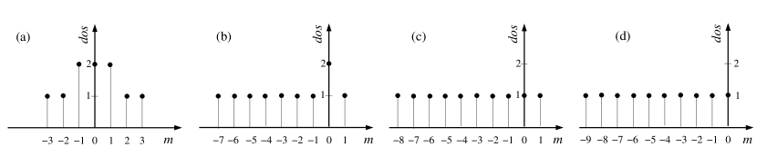
Figure 2: Density of occupied states (dos) as a function of the quantum number M = n_d – n_g for each of the configurations shown in Fig. 1.

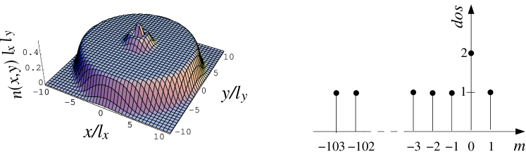
Figure 3: Density profile (left) and dos (right) for 106 fermions in a circular harmonic trap at $\omega_{L}$ = 5$\omega_{0}$.

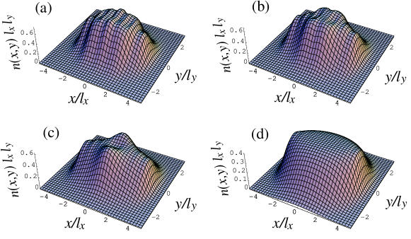
Figure 4: Density profile for 10 fermions in an elliptical harmonic trap with anisotropy parameter $\lambda$ = 4 at (a) $\omega_{L}$ = 0, (b) $\omega_{L}$ = $\omega_{0}$, (c) $\omega_{L}$ = 1.8$\omega_{0}$, and (d) $\omega_{L}$ = 10$\omega_{0}$.

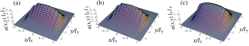
Figure 5: Density profile for 10 fermions in an elliptical harmonic trap with strong anisotropy ($\lambda$ = 10) at (a) $\omega_{L}$ = 0, (b) $\omega_{L}$ = $\omega_{0}$, and (c) $\omega_{L}$ = 10$\omega_{0}$.

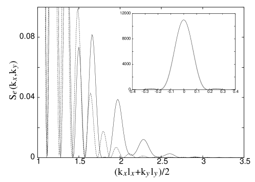
Figure 6: Elastic contribution to the static structure factor $S_{e}(k_{x},k_{y})$ corresponding to the spatial density distribution shown in Fig. 3 (continuous line) and to an MDD distribution of the same number of fermions (dashed line), as a function of $(k_{x}l_{x}+k_{y}l_{y})/2$ at $k_{x}l_{x}=k_{y}l_{y}$. The inset shows the central peak of the two patterns.

References

- [1] B. DeMarco and D.S. Jin, Science 285 (1999) 1703; M.O. Mewes, G. Ferrari, F. Schreck, A. Sinatra, and C. Salomon, Phys. Rev. A 61 (2000) 011403; C.A. Regal, M. Greiner, and D.S. Jin, Phys. Rev. Lett. 92 (2004) 040403; L. Pezzè, L. Pitaevskii, A. Smerzi, S. Stringari, G. Modugno, E. de Mirandes, F. Ferlaino, H. Ott, G. Roati, and M. Inguscio, Phys. Rev. Lett. 93 (2004) 120401.
- [2] For a recent review on confined quantum gases see A. Minguzzi, S. Succi, F. Toschi, M.P. Tosi, and P. Vignolo, Phys. Rep. 395 (2004) 223.
- [3] P. Vignolo, A. Minguzzi, and M.P. Tosi, Phys. Rev. Lett. 85 (2000) 2850.
- [4] F. Gleisberg, W. Wonneberger, U. Schlöder, and C. Zimmermann, Phys. Rev. A 62 (2000) 063602.
- [5] M. Brack and B.P. van Zyl, Phys. Rev. Lett. 86 (2001) 1574.
- [6] P. Vignolo and A. Minguzzi, Phys. Rev. A 67 (2003) 053601.
- [7] E.J. Mueller, Phys. Rev. Lett. 93 (2004) 190404.
- [8] M.A. Kastner, Phys. Today 46 (1993) 24.
- [9] T. Chakraborty, Quantum Dots: A Survey of the Properties of Artificial Atoms (Elsevier, Amsterdam, 1999).
- [10] L. Jacak, P. Hawrylak, and A. Wòjs, Quantum Dots (Springer, Berlin, 1998).
- [11] S. Tarucha, D.G. Austing, T. Honda, R.J. van der Hage, and L.P. Kouwenhoven, Phys. Rev. Lett. 77 (1996) 3613.
- [12] S.M. Reimann and M. Manninen, Rev. Mod. Phys. 74 (2002) 1283.
- [13] A.V. Madhav and T. Chakraborty, Phys. Rev. B 49 (1994) 8163.
- [14] P.S. Drouvelis, P. Semelcher, and F.K. Diakonos, J. Phys.: Condens. Matter 16 (2004) 3633.
- [15] B.P. van Zyl and D.A.W. Hutchinson, Phys. Rev. B 69 (2004) 024520.
- [16] H. Marmanis, Phys. Fluids 10 (1998) 1428; ibid. 3031.
- [17] Z.F. Ezawa, Quantum Hall Effects: Field Theoretical Approach and Related Topics (World Scientific, Singapore, 2000).
- [18] C. Cohen-Tannoudji, B. Diu, and F. Laloë, Mechanique Quantique (Hermann, Paris, 1998).
- [19] S. Tarucha, D.G. Austing, S. Sasaki, Y. Tokura, W. van der Wiel, and L.P. Kouwenhoven, Appl. Phys. A 71 (2000) 367.
- [20] P. Vignolo, A. Minguzzi, and M.P. Tosi, Phys. Rev. A 64 (2001) 023421.